In this section, the eight different vector styling types will be covered. The eight types are single symbol, categorized, graduated, rule-based, point-displacement, inverted polygons, heatmap, and 2.5 D.
Note that even though layer rendering is part of vector style properties, it will be discussed separately in the next section as it is common to all vector styling types.
The single-symbol vector style applies the same symbol to every record in the vector dataset. This vector style is best when you want a uniform look for a map layer, such as when you style lake polygons or airport points.
The following screenshot shows the Single Symbol style type with default parameters for point vector data. Its properties will be very similar to line and polygon vector data.
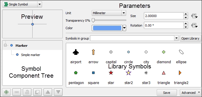
Let's take a quick tour of the four parts of the properties window for the Single Symbol style type shown in the previous screenshot:
- Symbol Preview, in the upper-left corner, shows a preview of a symbol with the current parameters.
- Symbol Parameters, in the upper-right corner, has the parameters for the symbol selected in the symbol component tree (these will change slightly depending on geometry type of the vector data).
- Library Symbols, in the bottom-right corner, lists a group of symbols from the library (which is also known as Style Manager). Clicking on a symbol sets it as the current symbol design. If symbol groups exist, they can be selected for viewing in the Symbols in group drop-down menu. To open the Style Manager, click on Open Library.
- Symbol Component Tree, in the bottom-left corner, lists the layers of symbol components. Clicking on each layer changes the symbol parameters so that the symbol can be changed.
Note
When you have a sub-component (Simple marker for example) selected in the symbol component tree, you have the option to enable Draw effects. These effects are covered in detail in Chapter 7, Advanced Data Visualization in the Learn to use live layer effects section.
As an example of how to use the Single Symbol style properties to create a circle around a gas pump ![]() , a second layer with the SVG marker symbol layer type was added by clicking on the Add symbol layer button (
, a second layer with the SVG marker symbol layer type was added by clicking on the Add symbol layer button (![]() ), and was then moved on top of the circle by clicking on the Move up button (
), and was then moved on top of the circle by clicking on the Move up button (![]() ). The following figure shows the parameters used to create the symbol:
). The following figure shows the parameters used to create the symbol:

To save your custom symbol to the Style Manager, click on the Save button to name and save the style. The saved style will appear in the Style Manager and the list of library symbols.
The categorized vector style applies one symbol per category of the attribute value(s). This vector style is the best when you want a different symbol that is based on attribute values, such as when styling country polygons or classes of roads lines. The categorized vector style works best with nominal or ordinal attribute data.
The following screenshot shows the Categorized style type with parameters for point vector data of schools. Its properties will be very similar to those for line and polygon vector data.
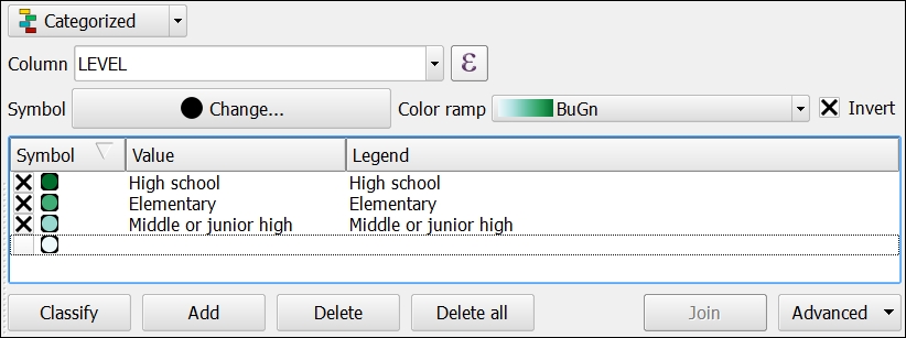
Styling vector data with the Categorized style type is a four-step process, which is as follows:
- Select an appropriate value for the Column field to use the attributes for categorization. Optionally, an expression can be created for categorization by clicking on the Expression button () to open the Expression dialog.
- Create the classes to list by either clicking on the Classify button to add a class for each unique attribute that is found; otherwise, click on the Add button to add an empty class and then double-click in the Value column to set the attribute value to be used to create the class. Classes can be removed with the Delete or Delete all buttons. They can be reordered by clicking and dragging them up and down the list. Classes can also be modified by double-clicking in the Value and Label columns.
- Set the symbol for all classes by clicking on the Symbol button to open the Symbol selector window. Individual class symbols can be changed by double-clicking on the Symbol column of the class list.
- Choose the color ramp to apply to the classes. Individual class colors can be changed by double-clicking on the Symbol column of the class list.
Other symbol options (which will change availability based on vector layer type), such as transparency, color, size, and output unit, are available by right-clicking on a category row. Additionally, advanced settings are available by clicking on the Advanced button.
The graduated vector style applies one symbol per range of numeric attribute values. This vector style is the best when you want a different symbol that is based on a range of numeric attribute values, such as when styling gross domestic product polygons or city population points. The graduated vector style works best with ordinal, interval, and ratio numeric attribute data.
The following screenshot shows the Graduated style type with parameters for polygon vector data of the populations of the states. Its properties will be very similar to that of point and line vector data.

Styling vector data with the Graduated style type is a five-step process, which is as follows:
-
Select an appropriate value for the Column field to use the attributes for classification. Optionally, an expression can be created for classification by clicking on the Expression button (
 ) to open the Expression dialog.
- Choose the number of classes and the classification mode. The following five modes are available for use:
- Equal Interval: In this mode, the width of each class is set to be the same. For example, if input values ranged between 1 and 100 and four classes were desired, then the class ranges would be 1-25, 26-50, 51-75, and 76-100 so that there are 25 values in each class.
- Quantile (Equal Count): In this mode, the number of records in each class is distributed as equally as possible, with lower classes being overloaded with the remaining records if a perfectly equal distribution is not possible. For example, if there are fourteen records and three classes, then the lowest two classes would contain five records each and the highest class would contain four records
- Natural Breaks (Jenks): The Jenks Breaks method maximizes homogeneity within classes and creates class breaks that are based on natural data trends.
- Standard Deviation: In this mode, classes represent standard deviations above and below the mean record values. Based on how many classes are selected, the number of standard deviations in each class will change.
- Pretty Breaks: This creates class boundaries that are round numbers to make it easier for humans to delineate classes.
- Create the classes to list by either clicking on the Classify button to add a class for each unique attribute that is found; otherwise, click on the Add Class button to add an empty class and then double-click in the Value column to set the attribute value range to be used to create the class. Classes can be removed with the Delete or Delete All buttons. They can be reordered by clicking and dragging them up and down the list. Classes can also be modified by double-clicking in the Value and Label columns.
- Set the symbol for all classes by clicking on the Symbol button to open the Symbol selector window. Individual class symbols can be changed by double-clicking on the Symbol column of the class list.
- Choose the Color ramp to apply to the classes. Individual class colors can be changed by double-clicking on the Symbol column of the class list.
The Legend Format field sets the format for all labels. Anything can be typed in the textbox. The lower boundary of the class will be inserted where %1 is typed in the textbox, and the upper boundary of the class will be inserted where %2 is typed.
If Link class boundaries is checked, then the adjacent class boundary values will be automatically changed to be adjacent if any of the class boundaries are manually changed.
Other symbol options, such as transparency, color, and output unit, are available by right-clicking on a category row. Advanced settings are available by clicking on the Advanced button.
The Histogram tab (shown in the following figure) allows you to visualize the distribution of the values in the selected column. It is often useful to view the histogram before you decide on the classification method to gain an overview of the distribution of the data and to quickly identify any outliers, skew, large gaps, or other characteristics that may affect your classification choice.
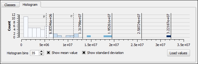
To view the data in the histogram, click on the Load values button. You can change the number of bars in the histogram by modifying the value in the Histogram bins box. You can view the mean and standard deviation by checking the Show mean value and Show standard deviation boxes, respectively.
The rule-based vector style applies one symbol per created rule and can apply maximum and minimum scales to toggle symbol visibility. This vector style is the best when you want a different symbol that is based on different expressions or when you want to display different symbols for the same layer at different map scales. For example, if you are styling roads, a rule could be set to make roads appear as thin lines when zoomed out, but when zoomed in, the thin lines will disappear and will be replaced by thicker lines that are more scale appropriate.
There are no default values for rule-based styling; however, if a style was previously set using a different styling type, the style will be converted to be rule-based when this style type is selected. The following screenshot shows the Categorized style type from the previous section that is converted to the Rule-based style type parameters for polygon vector data of the populations of the countries. Its properties will be very similar to that of point and line vector data.
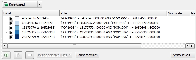
The Rule-based style properties window shows a list of current rules with the following columns:
- Label: The symbol and label that will be visible in the Layers panel are displayed here. The checkbox toggles rule activation; unchecked rules will not be displayed.
- Rule: This displays the filter applied to the vector dataset to select a subset of records.
- Min. Scale: This displays the smallest (zoomed-out) scale at which the rule will be visible.
- Max. Scale: This displays the largest (zoomed-in) scale at which the rule will be visible.
- Count: This displays the number of features that are included in this rule. This is calculated when the Count features button is clicked.
- Duplicate count: This displays the number of features that are included in the current and other rules. This is helpful when you are trying to achieve mutually exclusive rules and need to determine where duplicates exist. This is calculated when the Count features button is clicked.
To add a new rule, click on the Add rule button (![]() ) to open the Rule properties window. To edit a rule, select the rule and then click on the Edit rule button (
) to open the Rule properties window. To edit a rule, select the rule and then click on the Edit rule button (![]() ) to open the Rule properties window. To remove a rule, select the rule and then click on the Remove rule button (
) to open the Rule properties window. To remove a rule, select the rule and then click on the Remove rule button (![]() ).
).
Additional scales, categories, and ranges can be added to each rule by clicking on the Refine current rules button. To calculate the number of features included in each rule and to calculate the duplicate feature count, click on the Count features button.
When a rule is added or edited, the Rule properties window (which is shown in the next screenshot) displays five rule parameters, which are as follows:
- Label: This should have the rule label that will be displayed in the Layers panel.
- Filter: This will have the expression that will select a subset of features to include in the rule. Click on the ellipsis button to open the Expression string builder window. Then, click on the Test button to check the validity of the expression.
- Description: This has a user-friendly description of the rule.
- Scale range: This has the Minimum (exclusive) and Maximum (inclusive) scales between which the rule will be visible.
- Symbol: This has the symbol that will be used to symbolize features included in the rule.
None of the parameters are required (Label, Filter, and Description could be left blank); to exclude Scale range and Symbol from the rule, uncheck the boxes next to these parameters.
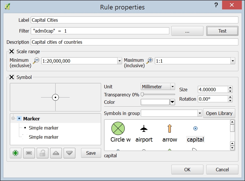
As an example of use, using the Populated Places.shp sample data, capital cities, megacities, and all other places can be styled differently by using rule-based styling. Additionally, each rule is visible to the minimum scale of 1:1, although they become invisible at different maximum scales. The following screenshot shows the rules created and a sample map of selected populated places in the country of Nigeria:

The point-displacement vector style radially displaces points that lie within a set distance from each other so that they can be individually visualized. This vector style works best on data where points may be stacked on top of each other, thereby making it hard to see each point individually. This vector style only works with the point vector geometry type.
The following screenshot shows how the Point Displacement style works by using the Single Symbol renderer, which is applied to the Stacked Points.shp sample data. Each point within the Point distance tolerance value of at least one other point is displaced at a distance of the Circle radius modification value around a newly-created center symbol. In this example, three groups of circles have been displaced around a center symbol.
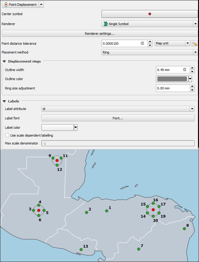
The Point Displacement style parameters, shown in the preceding figure, provide multiple parameters to displace the points, set the sub-renderer, style the center symbol, and label the displaced points. Let's review parameters that are unique to the point-displacement style:
- Center symbol: This contains the style for the center symbol that is created at the location from where the point symbols are being displaced.
- Renderer: This contains the renderer that styles the displaced points. Click on the Renderer settings button to access renderer settings.
- Point distance tolerance: For each point, if another point (or points) is within this distance tolerance, then all points will be displaced. The tolerance can be specified in millimeters, pixels, or map units. If choosing map units, further configuration becomes available allowing for displacement to only happen between certain scale ranges or at certain size ranges.
- Placement method: Sets the method of placing the displaced points as either Ring or Concentric rings.
- Outline width: This sets the outline pen width in millimeters that visualizes the displacement ring value.
- Outline color: This contains the outline pen color for the displacement ring.
- Ring size adjustment: The number of additional millimeters that the points are displaced from the center symbol.
The Labels parameters applies to all points (displaced or not) in the vector data. It is important to use these label parameters, rather than the label parameters on the Labels tab of the Layer Properties window, because the labels set in the Labels tab will label the center symbol and not the displaced points.
The inverted polygons vector style inverts the area that a polygon covers. This vector style only works with the polygon vector geometry type.
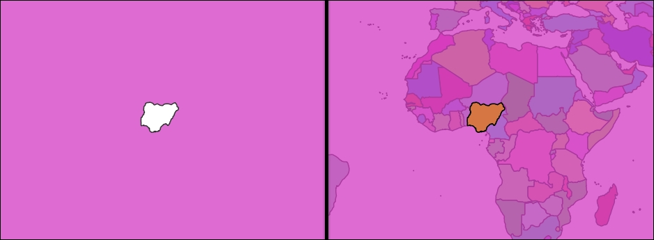
The following figure shows the Inverted polygons style for a polygon of the country of Nigeria on the left and all countries underneath the transparent inverted polygon of Nigeria on the right. Notice that the entire canvas is covered by the inverted polygon, which has the effect of cutting out Nigeria from the map.
The Inverted Polygons style parameters rely on a sub-renderer to determine the symbol used for the inverted polygons. By choosing the Sub renderer, the polygon rendering is inverted to cover the entire map canvas. The following screenshot shows the Inverted Polygons style parameters that created the inverted polygon of Nigeria:
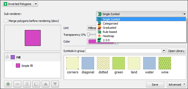
If multiple polygons are going to be inverted and the polygons overlap, Merge polygons before rendering (slow) can be checked so that the inverted polygons do not cover the area of overlap.
A heatmap represents the spatial density of points visualized across a color ramp. The heatmap vector style can only be applied to point or multipoint vector geometry types. As an example, the following figure uses a heatmap on a city population point layer to visualize the density and distribution of population in the United States of America:

To create a heatmap, open the style properties of a point vector file, and select Heatmap as the renderer. The heatmap vector renderer has five settings (shown in following figure) that determine how the heatmap will display:
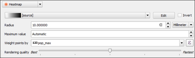
- Color ramp: Sets the color ramp that will be applied across the heatmap. The colors on the left-hand side of the color ramp will represent low density, and the colors on the right-hand side of the color ramp will represent high density. To reverse this, check Invert.
- Radius: The size of the circles that will be rendered on the heatmap. Choosing a larger radius will cause coalescence with nearby density circles. The radius can be set in Millimeter, Pixel, or Map Unit.
- Maximum value: Values that meet or exceed this value will be assigned the largest density circle size. This is useful when trying to bound the upper-end of the data so a very large outlier won't overly skew the heatmap to the largest values. This defaults to Automatic, which is the maximum value found in the Weight points by field. To set the Maximum value back to Automatic, enter a value of
0. - Weight points by: The numeric values in the chosen field will be used to weight the density calculation. Larger values will be weighted more heavily, resulting in denser circles.
- Rendering quality: Set on a sliding scale between Best and Fastest, this sets the quality of the rendering. The Best setting creates a smoother heatmap, but it renders slowly, and the Fastest setting creates a more pixelated heatmap, but renders quickly.
Rarely is the default heatmap satisfactory, so it is recommended to iterate through different values of the radius to create the most impactful and meaningful heatmap.
The 2.5 D vector style extrudes two-dimensional (flat) polygons to make them look like they are three-dimensional at a set view angle. This view style is also commonly known as two-thirds (2/3) view, perspective view, or two-and-one-half (2.5) view. Regardless of the name, the 2.5 D vector style can create some compelling scenes. As an example, the following figure shows a portion of a city where the buildings are styled using the 2.5 D vector style:
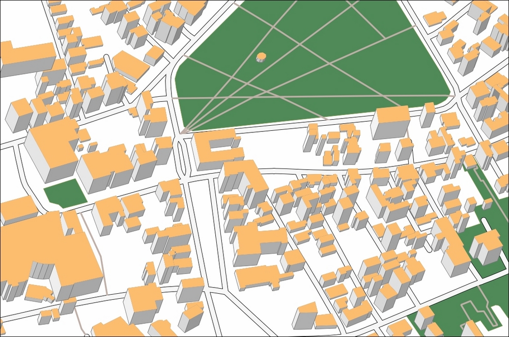
We will now explain the settings used to create this 2.5 D city map. First, a polygon vector layer must be added to the map canvas; in our case, this was a building polygon layer. Next, open the style properties and choose the 2.5 D renderer. The following image shows the settings available for the 2.5 D renderer:
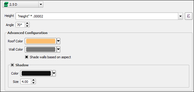
There are a number of settings available to the 2.5 D renderer. We will now examine each in detail:
- Height: This setting determines the height the polygons will be extruded, in map units. This can be either a number you enter, a field in the attribute table, or a calculation:
- If you enter a number, then all polygons will be extruded to this height.
- If you enter an attribute field, then the polygons will individually extrude to their associated value.
-
If you click on the Expression button (), then you can create an expression to be evaluated for the polygons' extrusion height. Often, the height value stored in attribute fields are in a different unit than the map unit and will need to be converted so the rendering is correct. For instance, if the map units are in meters, but the height attribute is in feet, then you would need to multiply the height attribute by 0.3048.
- Angle: The angle at which the extruded polygons will lean. The angle can be specified in values between 0 degrees and 359 degrees, with the default being 70 degrees. 0 degrees is the right of the screen and increases in a counter-clockwise direction, so that 90 degrees is the top of your screen.
- Advanced Configuration: This section of settings allows you to set the Roof Color (top of extruded polygon), Wall Color (sides of extruded polygon), and toggle Shade walls based on aspect. The shading varies the value of the wall colors to simulate shade from a light source. Turning off shading causes the walls to be rendered in the chosen, single, flat Wall Color.
- Shadow: If this is enabled, a shadow using the set Color and with the set Size will appear around the base of the extruded polygons.
Using the 2.5 D renderer is pretty easy and straightforward, but a neat feature is that it can be combined with another renderer (single, categorized, or graduated), which allows the extruded polygons to have different colors based on the second renderer used. To combine renderers, you must first render with the 2.5 D renderer, Apply the renderer, then change the renderer, set the second renderer's settings, and then Apply again. The only downside to combining renders is that the roof and wall colors are set to the same color value, as shown in the following image:

The eight vector layer styles really provide a great deal of control over the way your data is displayed on the map canvas. A number of vector layer styles have been added in recent releases of QGIS and have really increased the cartographic capabilities of the software. Speaking of great improvements to cartographic capabilities, the next section covers layer rendering, which really allows for some great visual effects to be added to your map!