
Chapter 22
Editing and Visualizing 3D Solids
In the previous 3D chapters, you spent some time becoming familiar with the AutoCAD 3D modeling features. In this chapter, you’ll focus on 3D solids and how they’re created and edited. You’ll also learn how you can use some special visualization tools to show your 3D solid in a variety of ways.
You’ll create a fictitious mechanical part to explore some of the ways you can shape 3D solids. This will also give you a chance to see how you can turn your 3D model into a standard 2D mechanical drawing. In addition, you’ll learn about the 3D solid editing tools that are available through the Tool Sets palette and the menu bar.
In this chapter, you’ll learn to do the following:
- Understand solid modeling
- Create solid forms
- Create complex solids
- Edit solids
- Streamline the 2D drawing process
- Visualize solids
Solid modeling is a way of defining 3D objects as solid forms. When you create a 3D model by using solid modeling, you start with the basic forms of your model—cubes, cones, and cylinders, for example. These basic solids are called primitives. Then, using more of these primitives, you begin to add to or subtract from your basic forms.
For example, to create a model of a tube, you first create two solid cylinders, one smaller in diameter than the other. You then align the two cylinders so that they’re concentric and tell AutoCAD to subtract the smaller cylinder from the larger one. The larger of the two cylinders becomes a tube whose inside diameter is that of the smaller cylinder, as shown in Figure 22-1. Several primitives are available for modeling solids in AutoCAD (Figure 22-2).
You can join these shapes—polysolid, box, wedge, cone, sphere, cylinder, pyramid, and donut (or torus)—in one of four ways to produce secondary shapes. The first three, demonstrated in Figure 22-3 using a cube and a cylinder as examples, are called Boolean operations. (The name comes from the nineteenth-century mathematician George Boole.)
The three Boolean operations are as follows:
Intersection Uses only the intersecting region of two objects to define a solid shape
Subtraction Uses one object to cut out a shape in another
Union Joins two primitives so they act as one object
The fourth option, interference, lets you find exactly where two or more solids coincide in space—similar to the results of a union. The main difference between interference and union is that interference enables you to keep the original solid shapes, whereas union discards the original solids, leaving only their combined form. With interference, you can have AutoCAD either show you the shape of the coincident space or create a solid based on the shape of the coincident space.
Joined primitives are called composite solids. You can join primitives to primitives, composite solids to primitives, and composite solids to other composite solids.
Now let’s look at how you can use these concepts to create models in AutoCAD.
Figure 22-1:Creating a tube by using solid modeling
Figure 22-2:The solid primitives

Figure 22-3:The intersection, subtraction, and union of a cube and a cylinder

Exercise Examples Are “Unitless”
To simplify the exercises in this chapter, the instructions don’t specify inches or centimeters. This way, users of both the metric and Imperial measurement systems can use the exercises without having to read through duplicate information.
In the following sections, you’ll begin to draw the object shown later in the chapter in Figure 22-18. In the process, you’ll explore the creation of solid models by creating primitives and then setting up special relationships between them.
Primitives are the basic building blocks of solid modeling. At first, it may seem limiting to have only eight primitives to work with, but consider the varied forms you can create with just a few two-dimensional objects. Let’s begin by creating the basic mass of your steel bracket.
First, prepare your drawing for the exercise:
1. Open the file called Bracket.dwg. This file contains some objects that you’ll use in the first half of this chapter to build a 3D solid shape.
2. Make sure the Tool Sets palette shows the Modeling tool set.
3. Close the Material Browser if it is open.
Joining Primitives
In this section, you’ll merge the two box objects. First, you’ll move the new box into place. Then you’ll join the two boxes to form a single solid:
1. Click the Move tool, pick the smaller of the two boxes, and then press ↵.
2. Use the Midpoint osnap, and pick the middle of the front edge of the smaller box, as shown in the top image in Figure 22-4.
3. Use the Midpoint osnap to pick the middle of the bottom edge of the larger box, as shown in the bottom image in Figure 22-4.
4. Click the Union tool in the upper part of the Tool Sets palette, or type UNI↵.
Figure 22-4:Moving the smaller box
5. Click both boxes and press ↵. Your drawing now looks like Figure 22-5.
Figure 22-5:The two boxes joined

As you can see in Figure 22-5, the form has joined to appear as one object. It also acts like one object when you select it. You now have a composite solid made up of two box primitives.
Now let’s place some holes in the bracket. In this next exercise, you’ll discover how to create negative forms to cut portions out of a solid:
1. Turn on the layer called Cylinder. Two cylinder solids appear in the model, as shown in Figure 22-6. These cylinders are 1.5 units tall.
Figure 22-6:The cylinders appear when the Cylinder layer is turned on.

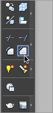
2. Click and hold the Union tool in the Tool Sets palette and click the Subtract tool from the flyout (Figure 22-7), or type SU↵.
Figure 22-7:The Subtract tool on the Union flyout

3. At the Select solids, surfaces, and regions to subtract from… Select objects: prompt, pick the composite solid of the two boxes and press ↵.
4. At the Select solids, surfaces, and regions to subtract… Select objects: prompt, click the two cylinders and press ↵. The cylinders are subtracted from the bracket.
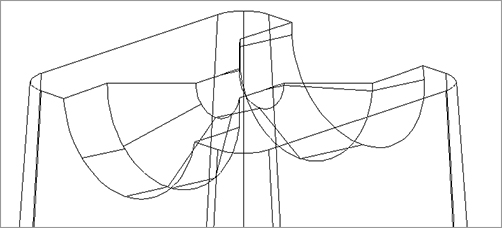
5. To temporarily view the solid with hidden lines removed, choose View Hide. You see a hidden-line view of the solid, similar to the one shown in Figure 22-8.
Figure 22-8:The bracket so far, with hidden lines removed

As you learned in the earlier chapters in Part 4, Wireframe views, such as the one in the previous exercise, are somewhat difficult to decipher. Until you use the Hide command (View Hide), you can’t be sure that the subtracted cylinders are in fact holes. Using the Hide command frequently will help you keep track of what’s going on with your solid model. You can also use a visual style like Hidden or Shades Of Gray.
You may also have noticed in step 4 that even though the cylinders were taller than the opening they created, they worked fine to remove part of the rectangular solid. The cylinders were 1.5 units tall, not 1 unit, which is the thickness of the bracket. Having drawn the cylinders taller than needed, you saw that when AutoCAD performed the subtraction, it ignored the portion of the cylinders that didn’t affect the bracket. AutoCAD always discards the portion of a primitive that isn’t used in a subtract operation.
Using 3D Solid Operations on 2D Drawings
You can apply some of the features described in this chapter to 2D drafting by taking advantage of AutoCAD’s region object. Regions are two-dimensional objects to which you can apply Boolean operations.
The following illustration shows how a set of closed polyline shapes can be quickly turned into a drawing of a wrench using regions. The shapes at the top of the figure are first converted into regions using the Region tool on the Closed Shapes tool group. Next, the shapes are aligned, as shown in the middle of the image. Finally, the circles and rectangle are joined with the Union command (type UNI↵); then, the hexagonal shapes are subtracted from the combined shape (type SU↵). You can use the Region.dwg sample file if you’d like to experiment.

You can use regions to generate complex surfaces that may include holes or unusual bends.

Keep in mind the following:
- Regions act like surfaces; when you remove hidden lines, objects behind the regions are hidden.
- You can explode regions to edit them. However, exploding a region causes the region to lose its surfacelike quality, and objects no longer hide behind its surface(s).
- You can
 -click the edge of a region to edit a region’s shape.
As you learned earlier, you can convert a polyline into a solid by using the Extrude tool on the Tool Sets palette. This process lets you create more-complex shapes than the built-in primitives. In addition to the simple straight extrusion you’ve already tried, you can extrude shapes into curved paths or you can taper an extrusion.
Tapering an Extrusion
Let’s look at how you can taper an extrusion to create a fairly complex solid with little effort:
1. Turn on the Taper layer. A rectangular polyline appears. This rectangle has its corners rounded to a radius of 0.5 using the Fillet command.
2. Click the Extrude tool near the top of the Tool Sets palette, or enter EXT↵ at the Command prompt.
3. At the Select objects to extrude or [MOde]: prompt, pick the polyline on the Taper layer and press ↵.
4. At the Specify height of extrusion or [Direction/Path/Taper angle/Expression]: prompt, enter T↵.
5. At the Specify angle of taper for extrusion or [Expression] <0>: prompt, enter 4↵.
6. At the Specify height of extrusion or [Direction/Path/Taper angle/Expression]: prompt, point the cursor upward and enter 3↵. The extruded polyline looks like Figure 22-9.
Figure 22-9:The extruded polyline

7. Join the part you just created with the original solid. Click the Union tool on the Tool Sets palette or type UNI↵.
8. Click the extruded part and the composite solid just below it. Press ↵ to complete your selection.
In step 5, you can indicate a taper for the extrusion. Specify a taper in terms of degrees from the Z axis, or enter a negative value to taper the extrusion outward. You can also press ↵ to accept the default of 0° to extrude the polyline without a taper.
What Are Isolines?
You may have noticed the message in the Command Line palette that reads as follows:
Current wire frame density: ISOLINES=4
This message tells you the current setting for the Isolines system variable. This variable controls the way curved objects, such as cylinders and holes, are displayed. A setting of 4 causes a cylinder to be represented by four lines with a circle at each end. You can see this in the holes that you created for the Bracket model in the previous exercise. You can change the Isolines setting by entering ISOLINES↵ at the Command prompt. You then enter a value for the number of lines to use to represent surfaces. This setting is also controlled by the Contour Lines Per Surface option in the Document Settings tab of the Application Preferences dialog box.
Sweeping a Shape on a Curved Path
As you’ll see in the following exercise, the Sweep command lets you extrude virtually any polyline shape along a path defined by a polyline, an arc, or a 3D polyline. At this point, you’ve created the components needed to do the extrusion. Next, you’ll finish the extruded shape:
1. Turn on the Path layer. This layer contains the circle you’ll extrude and the polyline path, which looks like an S, as shown in Figure 22-10.
2. Click the Sweep tool from the Revolve flyout, or type SWEEP↵. Click the circle, and then press ↵.
Figure 22-10:Hidden-line view showing parts of the drawing you’ll use to create a curved extrusion

3. At the Select sweep path or [Alignment/Base point/Scale/Twist]: prompt, click the polyline curve.
4. AutoCAD generates a solid tube that follows the path. The tube may not look like a tube because AutoCAD draws extruded solids such as this with four lines showing their profile.
5. Click the Subtract tool from the Union flyout on the Tool Sets palette or type SU↵, and then select the composite solid.
6. Press ↵. At the Select objects: prompt, click the curved solid you just created and press ↵. The curved solid is subtracted from the square solid.
7. Choose View Hide. Your drawing looks like Figure 22-11.
Figure 22-11:The solid after subtracting the curve

In this exercise, you used a curved polyline for the extrusion path, but you can use any type of 2D or 3D polyline, as well as a line or arc, for an extrusion path.
Revolving a Polyline
When your goal is to draw a circular object, you can use the Revolve tool in the Tool Sets palette to create a solid that is revolved, or swept in a circular path. Think of Revolve’s action as similar to a lathe that lets you carve a shape from an object on a spinning shaft. In this case, the object is a polyline, and rather than carve it, you define the profile and then revolve the profile around an axis.
In the following exercise, you’ll draw a solid that will form a slot in the tapered solid. A 2D polyline that is the profile of the slot has been created for you. You’ll simply use cut and paste to bring the polyline into the bracket drawing:
1. Select 2D Wireframe from the Visual Styles menu on the Viewport Controls.
2. Zoom in to the top of the tapered box so you have a view similar to Figure 22-12.
Figure 22-12:An enlarged view of the top of the tapered box and pasted polyline
3. Turn on the Revolve layer. This layer contains a closed polyline that you’ll use to create a cylindrical shape.
4. Click the Revolve tool on the Tool Sets palette, or type REV↵ at the Command prompt.
5. At the Select objects to revolve or [MOde]: prompt, pick the polyline on the top of the tapered surface and press ↵.
6. When you see the prompt
Specify axis start point or define axis by [Object/X/Y/Z] <Object>:
use the Endpoint osnap override and pick the beginning corner endpoint of the polyline you just added, as shown in Figure 22-12.
7. At the Specify axis endpoint: prompt, pick the axis endpoint indicated in Figure 22-12.
8. At the Specify angle of revolution or [STart angle/Reverse/eXpression] <360>: prompt, press ↵ to sweep the polyline a full 360°. The revolved form appears, as shown in Figure 22-13.
Figure 22-13:The revolved polyline

You just created a revolved solid that will be subtracted from the tapered box to form a slot in the bracket. However, before you subtract it, you need to make a slight change in the orientation of the revolved solid:
1. Choose Modify 3D Operations 3D Rotate on the menu bar, or type 3DROTATE↵. You see the following prompt:
Current positive angle in UCS: ANGDIR=counterclockwise ANGBASE=0
Select objects:
2. Select the revolved solid and press ↵.
3. At the Specify base point: prompt, use the Midpoint osnap and click the right side edge of the top surface, as shown in Figure 22-14.
Figure 22-14:Selecting the points to rotate the revolved solid in 3D space
4. At the Pick a rotation axis: prompt, point to the green rotation grip. When you see a green line appear along the Y axis, click the mouse.
5. At the Specify angle start point or type an angle: prompt, enter -5↵ for a minus 5 degrees rotation. The solid rotates 5° about the Y axis.
6. Click the Subtract tool from the Union flyout, or type SU↵. Click the tapered box, and then press ↵.
7. At the Select objects: prompt, click the revolved solid and press ↵. Your drawing looks like Figure 22-15.
Figure 22-15:The composite solid
Basic solid forms are fairly easy to create. Refining those forms requires some special tools. In the following sections, you’ll learn how to use familiar 2D editing tools, as well as some new tools, to edit a solid. You’ll also be introduced to the Slice tool, which lets you cut a solid into two pieces.
Splitting a Solid into Two Pieces
One of the more common solid-editing tools you’ll use is the Slice tool. As you may guess from its name, Slice enables you to cut a solid into two pieces. The following exercise demonstrates how it works:
1. Choose View Zoom All to get an overall view of your work so far.
2. Click the Slice tool from the Solids – Edit tool group (Figure 22-16), or type SL↵.
3. At the Select objects to slice: prompt, click the model and press ↵. Note that if you need to, you could select more than one solid at this prompt. The Slice command would then slice all the solids through the plane indicated in steps 4 and 5. For now, you’re just selecting one solid.
Figure 22-16:The Slice tool on the Solids – Edit tool group

4. At the prompt
Specify start point of slicing plane or
[planar Object/Surface/Zaxis/View/XY/YZ/ZX/
3points] <3points>:
type XY↵. This lets you indicate a slice plane parallel to the XY plane.
5. At the Specify a point on the XY-plane <0,0,0>: prompt, type 0,0,0.5↵. This places the slice plane at the Z coordinate of 0.5 units. You can also use the Midpoint osnap and pick any vertical edge of the rectangular base of the solid. If you want to delete one side of the sliced solid, you can indicate the side you want to keep by clicking it in step 6 instead of entering B↵.
6. At the Specify a point on desired side or [keep Both sides]: prompt, type B↵ to keep both sides of the solid. AutoCAD divides the solid horizontally, one-half unit above the base of the part as shown in Figure 22-17.
Figure 22-17:The solid sliced through the base
In step 4, you saw a number of options for the Slice command. You may want to make note of those options for future reference. Table 22-1 provides a list of the options and their purposes.
Table 22-1: Slice command options
| Option | Purpose |
| planar Object | Lets you select an object to define the slice plane. |
| Surface | Lets you select a surface object to define the shape of a slice (see Chapter 20, “Using Advanced 3D Features”). |
| Zaxis | Lets you select two points defining the Z axis of the slice plane. The two points you pick are perpendicular to the slice plane. |
| View | Generates a slice plane that is perpendicular to your current view. You’re prompted for the coordinate through which the slice plane must pass—usually a point on the object. |
| XY/YZ/ZX | Pick one of these to determine the slice plane based on the X, Y, or Z axis. You’re prompted to pick a point through which the slice plane must pass. |
| 3points | The default setting; lets you select three points defining the slice plane. Normally, you pick points on the solid. |
Rounding Corners with the Fillet Tool
Your bracket has a few sharp corners that you may want to round in order to give it a more realistic appearance. You can use the Tool Sets palette’s Fillet and Chamfer tools to add these rounded corners to your solid model:
1. Click the Fillet tool in the middle of the lower half of the Tool Sets palette or type F↵.
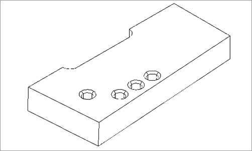
2. At the Select first object or [Undo/Polyline/Radius/Trim/Multiple]: prompt, pick the edge indicated in the first image in Figure 22-18.
3. At the Enter fillet radius or [Expression] <0.5000>: prompt, type 0.2↵.
4. At the Select an edge or [Chain/Radius]: prompt, type C↵ for the Chain option. Chain lets you select a series of solid edges to be filleted.
5. Select one of the other seven edges at the base of the tapered form and press ↵.
6. Type HIDE↵ to get a quick look at your model in a hidden line view, as shown in the second image in Figure 22-18.
As you saw in step 4, Fillet acts a bit differently when you use it on solids. The Chain option lets you select a set of edges instead of just two adjoining objects.
Figure 22-18:Filleting solids

Chamfering Corners with the Chamfer Tool
Now let’s try chamfering a corner. To practice using Chamfer, you’ll add a countersink to the cylindrical hole you created in the first solid:
1. Type REGEN↵ to return to a wireframe view of your model.
2. Click the Chamfer tool (Figure 22-19), which is next to the Fillet tool on the Tool Sets palette, or type Cha↵.
Figure 22-19:Click the Chamfer tool.
3. At the prompt
Select first line or [Undo/Polyline/Distance/Angle/Trim/mEthod/Multiple]:
pick the edge of the hole, as shown in Figure 22-20. Notice that the top surface of the solid is highlighted and that the prompt changes to Enter surface selection option [Next/OK (current)] <OK>:. The highlighting indicates the base surface, which will be used as a reference in step 5. (You could also type N↵ to choose the other adjoining surface, the inside of the hole, as the base surface.)
Figure 22-20:Picking the edge to chamfer
4. Press ↵ to accept the current highlighted face.
5. At the Specify base surface chamfer distance or [Expression] <0.1250>: prompt, type 0.125↵. This indicates that you want the chamfer to have a width of 0.125 across the highlighted surface.
6. At the Specify other surface chamfer distance or [Expression] <0.2000>: prompt, type 0.2↵.
7. At the Select an edge or [Loop]: prompt, click the top edges of both holes, and then press ↵. When the Chamfer command has completed its work, your drawing looks like Figure 22-21.
8. After reviewing the work you’ve done here, save the Bracket.dwg file.
The Loop option in step 7 lets you chamfer the entire circumference of an object. You don’t need to use it here because the edge forms a circle. The Loop option is used when you have a rectangular or other polygonal edge you want to chamfer.
Figure 22-21:The chamfered edges

Using the Solid Editing Tools
You’ve added some refinements to the Bracket model by using standard AutoCAD editing tools. There is a set of tools that is specifically geared toward editing solids. You already used the Union and Subtract tools found in the Solids – Edit tool group. In the following sections, you’ll explore some of the other tools in that tool group.
You don’t have to perform the exercises, but reviewing them will show you what’s available. When you’re more comfortable working in 3D, you may want to come back and experiment with the file called solidedit.dwg shown in the figures in the following sections.
Parallel Projection Needed for Some Features
Many of the features discussed in these sections work only in a parallel projection view. You can switch to a parallel projection view by choosing the 2D Wireframe visual style, or, if you have the ViewCube turned on, right-click the ViewCube and select Parallel. You can also choose Parallel from the 3D Views menu on the Viewport Controls.
Moving a Surface
You can move any flat surface of a 3D solid by choosing Modify Solid Editing Move Faces. When you choose this option, you’re prompted to select faces. Because you can select only the edge of two joining faces, you must select an edge and then use the Remove option to remove one of the two selected faces from the selection set (Figure 22-22). Once you’ve made your selection, press ↵. You can then specify a distance for the move.
After you’ve selected the surface you want to move, Move Faces acts just like the Move command: You select a base point and a displacement. Notice how the curved side of the model extends its curve to meet the new location of the surface. This shows you that AutoCAD attempts to maintain the geometry of the model when you make changes to the faces.
Figure 22-22:To select the vertical surface to the far right of the model, click the edge and then use the Remove option to remove the top surface from the selection.

Move Faces also lets you move entire features, such as the hole in the model. In Figure 22-23, one of the holes has been moved so that it’s no longer in line with the other three. This was done by selecting the countersink and the hole while using the Move Faces option.
Figure 22-23:Selecting a surface to offset

If a solid’s History setting is enabled, you can ![]() -click on its surface to expose the surface’s grip. You can then use the grip at the center of the surface to move the surface.
-click on its surface to expose the surface’s grip. You can then use the grip at the center of the surface to move the surface.
Offsetting a Surface
Suppose you want to decrease the radius of the arc in the right corner of the model and you also want to thicken the model by the same amount as the decrease in the arc radius. To do this, you can use the Offset Faces tool in the Solids – Edit tool group of the Tool Sets palette or choose Modify Solid Editing Offset Faces. The Offset Faces tool and the Offset command you used earlier in this book perform similar functions. The difference is that the Offset Faces tool affects 3D solids.
When you click the Offset Faces tool or choose Modify Solid Editing Offset Faces, you’re prompted to select faces. As with the Move Faces option, you must select an edge that will select two faces. If you want to offset only one face, you must use the Remove option to remove one of the faces. In Figure 22-23, an edge is selected. Figure 22-24 shows the effect of the Offset Faces tool when both faces are offset.
Figure 22-24:The model after offsetting the curved and bottom surfaces

Deleting a Surface
Now suppose you’ve decided to eliminate the curved part of the model. You can delete a surface by choosing Modify Solid Editing Delete Faces from the menu bar. Once again, you’re prompted to select faces. Typically, you’ll want to delete only one face, such as the curved surface in the example model. You use the Remove option to remove the adjoining face that you don’t want to delete before finishing your selection of faces to remove.
When you attempt to delete surfaces, keep in mind that the surface you delete must be recoverable by other surfaces in the model. For example, you can’t remove the top surface of a cube, expecting it to turn into a pyramid. That would require the sides to change their orientation, which isn’t allowed in this operation. You can, on the other hand, remove the top of a box with tapered sides. Then, when you remove the top, the sides converge to form a pyramid.
Rotating a Surface
All the surfaces of the model are parallel or perpendicular to each other. Imagine that your design requires two sides to be at an angle. You can change the angle of a surface by choosing Modify Solid Editing Rotate Faces on the menu bar.
As with the prior solid-editing tools, you’re prompted to select faces. You must then specify an axis of rotation. You can either select a point or use the default of selecting two points to define an axis of rotation, as shown in Figure 22-25. Once the axis is determined, you can specify a rotation angle. Figure 22-26 shows the result of rotating the two front-facing surfaces 4°.
Figure 22-25:Defining the axis of rotation

Figure 22-26:The model after rotating two surfaces
Tapering a Surface
In an earlier exercise, you saw how to create a new tapered solid by using the Extrude command. But what if you want to taper an existing solid? Here’s what you can do.
The Taper Faces tool from the Solids – Edit tool group prompts you to select faces. You can select faces, as described for the previously discussed solid-editing tools, using the Remove or Add option (Figure 22-27). Press ↵ when you finish your selection, and then indicate the axis from which the taper is to occur. In the model example in Figure 22-27, select two corners defining a vertical axis. Finally, enter the taper angle. Figure 22-28 shows the model tapered at a 4° angle.
Figure 22-27:Selecting the surfaces to taper and indicating the direction of the taper

Figure 22-28:The model after tapering the sides

Extruding a Surface
You’ve used the Extrude tool to create two of the solids in the Bracket model. The Extrude tool requires a closed polyline as a basis for the extrusion. As an alternative, the Solids – Edit tool group offers the Extrude Faces tool, which extrudes a surface of an existing solid.
When you click the Extrude Faces tool from the Solids – Edit tool group or type SOLIDEDIT↵ F↵ E↵, you see the Select faces or [Undo/Remove]: prompt. Select an edge or a set of edges or use the Remove or Add option to select the faces you want to extrude. Press ↵ when you’ve finished your selection, and then specify a height and taper angle. Figure 22-29 shows the sample model with the front surface extruded and tapered at a 45° angle. You can extrude multiple surfaces simultaneously if you need to by selecting them.
Figure 22-29:The model with a surface extruded and tapered

Aside from those features, the Extrude Faces tool works just like the Extrude command.
Turning a Solid into a Shell
In many situations, you’ll want your 3D model to be a hollow mass rather than a solid mass. The Shell option on the menu bar lets you convert a solid into a shell.
When you choose Modify Solid Editing Shell, or type SOLIDEDIT↵ B↵ S↵, you’re prompted to select a 3D solid. You’re then prompted to remove faces. At this point, you can select an edge of the solid to indicate the surface you want removed. The surface you select is completely removed from the model, exposing the interior of the shell. For example, if you select the front edge of the sample model shown in Figure 22-30, the top and front surfaces are removed from the model, revealing the interior of the solid, as shown in Figure 22-31. After selecting the surfaces to remove, you can enter a shell offset distance.
Figure 22-30:Selecting the edge to be removed

Figure 22-31:The solid model after using the Shell option

The shell thickness is added to the outside surface of the solid. When you’re constructing your solid with the intention of creating a shell, you need to take this into account.
Copying Faces and Edges
At times, you may want to create a copy of a surface of a solid to analyze its area or to produce another part that mates to that surface. The Modify Solid Editing Copy Faces option creates a copy of any surface on your model. The copy it produces is a type of object called a region.
The copies of the surfaces are opaque and can hide objects behind them when you perform a hidden-line removal (type HIDE↵).
Another menu bar option that is similar to Copy Faces is Copy Edges, which can be found by choosing Modify Solid Editing Copy Edges. Instead of selecting surfaces as in the Copy Faces tool, you select all the edges you want to copy. The result is a series of simple lines representing the edges of your model. This option can be useful if you want to convert a solid into a set of 3D Faces. The Copy Edges option creates a framework onto which you can add 3D Faces.
Adding Surface Features
If you need to add a feature to a flat surface, you can do so with the Modify Solid Editing Imprint Edges option. An added surface feature can then be colored using the Modify Solid Editing Color Faces option or extruded using the Presspull tool near the top of the Tool Sets palette. This feature is a little more complicated than some of the other solid-editing tools, so you may want to try the following exercise to see firsthand how it works.
You’ll start by inserting an object that will be the source of the imprint. You’ll then imprint the main solid model with the object’s profile:
1. Choose Insert Block from the menu bar to open the Insert Block dialog box, or type I↵.
2. Click Browse, and then locate the imprint.dwg sample file and select it.
3. In the Insert Block dialog box, make sure the Explode Block check box is selected.
4. Click Insert, then enter 0,0↵ for the insertion point and press ↵ to finish inserting the block. The block appears in the middle of the solid.
5. Choose Modify Solid Editing Imprint Edges or type IMPRINT↵.
6. Click the main solid model.
7. Click the inserted solid.
8. At the Delete the source object [Yes/No]<N>: prompt, enter Y↵↵.
You now have an outline of the intersection between the two solids imprinted on the top surface of your model. The imprint is really a set of edges that have been added to the surface of the solid. To help the imprint stand out, try the following steps to change its color:
1. Choose Modify Solid Editing Color Faces, or type SOLIDEDIT↵ F↵ L↵.
2. Click the imprint from the previous exercise. The imprint and the entire top surface are highlighted.
3. At the Select faces or [Undo/Remove/ALL]: prompt, type R↵; then click the outer edge of the top surface to remove it from the selection set.
4. Press ↵ to open the Color Palette dialog box.
5. Click the red color sample in the dialog box, and then click OK. The imprint is now red.
6. Press ↵ twice to exit the command.
7. To see the full effect of the Color Faces option, choose the Conceptual or Realistic visual style from the Visual Styles menu in the Viewports Control.
If you want to remove an imprint from a surface, ![]() -click the imprint and press the Delete key.
-click the imprint and press the Delete key.
Separating a Divided Solid
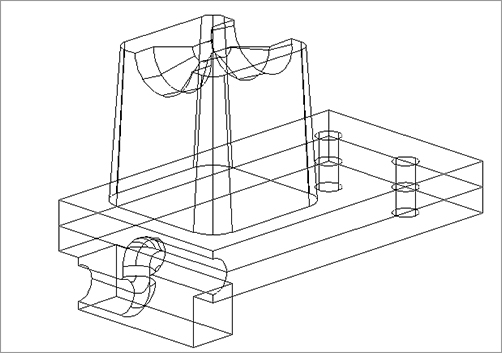
While editing solids, you can end up with two separate solid forms that were created from one solid, as shown in Figure 22-32. Even though the two solids appear separated, they act like a single object. In these situations, AutoCAD offers the Modify Solid Editing Separate option. Choose this option or type SOLIDEDIT↵ B↵ P↵ and select the solid that has been separated into two forms.
Figure 22-32:When the tall, thin solid is subtracted from the larger solid, the result is two separate forms, yet they still behave as a single object.
Using the Command Line for Solid Editing
The solid-editing tools are options of a single AutoCAD command called Solidedit. If you prefer to use the keyboard, here are some tips on using the Solidedit command. When you first enter SOLIDEDIT↵ at the Command prompt, you see the following prompt:
Enter a solids editing option [Face/Edge/Body/Undo/eXit] <eXit>:
You can select the Face, Edge, or Body option to edit the various parts of a solid. If you select Face, you see the following prompt:
Enter a face editing option [Extrude/Move/Rotate/Offset/Taper/
Delete/Copy/coLor/mAterial/Undo/eXit] <eXit>:.
The options from this prompt produce the same results as their counterparts on the Solid Editing panel.
If you select Edge at the first prompt, you see the following prompt:
Enter an edge editing option [Copy/coLor/Undo/eXit] <eXit>:.
The Copy option lets you copy a surface, and the coLor option lets you add color to a surface.
If you select Body from the first prompt, you see the following prompt:
Enter a body editing option [Imprint/seParate solids/Shell/
cLean/Check/Undo/eXit] <eXit>:.
These options also perform the same functions as their counterparts on the Solids – Edit tool group or the Modify Solid Editing menu option. As you work with this command, you can use the Undo option to undo the last Solidedit option you used without exiting the command.
Figure 22-32 is included in the sample figures at www.sybex.com/go/masteringautocadmac under the name Separate example.dwg. You can try the Separate option in this file on your own.
Through some simple examples, you’ve seen how each of the solid-editing tools works. You aren’t limited to using these tools in the way they were demonstrated in this chapter, and this book can’t anticipate every situation you might encounter as you create solid models. These examples are intended as an introduction to these tools, so feel free to experiment with them. You can always use the Undo option to backtrack in case you don’t get the results you expect.
This concludes your tour of the solid-editing tools. Next you’ll learn how to use 3D solid models to generate 2D working drawings quickly.
Finding the Properties of a Solid
All this effort to create a solid model isn’t designed just to create a pretty picture. After your model is drawn and built, you can obtain information about its physical properties.
You can find the volume, the moment of inertia, and other physical properties of your model by using the Massprop command. These properties can also be recorded as a file on disk, so you can modify your model without worrying about losing track of its original properties.
To find the mass properties of a solid, enter MASSPROP↵, and then follow the prompts.
Streamlining the 2D Drawing Process
Using solids to model a part—such as with the bracket and Solidedit examples in this chapter—may seem a bit exotic, but there are definite advantages to modeling in 3D, even if you only want to draw the part in 2D as a page in a set of manufacturing specs.
The exercises in the following sections show you how to generate a typical mechanical drawing from your 3D model quickly by using Paper Space and the solid-editing tools. You’ll also examine techniques for dimensioning and including hidden lines.
Architectural Elevations from 3D Solids
If your application is architecture and you’ve created a 3D model of a building by using solids, you can use the tools described in the following sections to generate 2D elevation drawings from your 3D solid model.
You might use solid models to generate 2D line drawings of elevations. Such line drawings can be “rendered” in a 2D drawing program like Adobe Photoshop or Illustrator. Be aware that such drawings will not be as accurate as those drawn from scratch, but they are fine for the early stages of a design project.
Drawing Standard Top, Front, and Right-Side Views
One of the most common types of mechanical drawings is the orthogonal projection. This style of drawing shows separate top, front, and right-side views of an object. Sometimes a 3D image is added for clarity. You can derive such a drawing in a few minutes using the Flatshot tool described in Chapter 19 (see the section “Turning a 3D View into a 2D AutoCAD Drawing”).
With Flatshot, you can generate the standard top, front, and right-side orthogonal projection views, which you can further enhance with dimensions, hatch patterns, and other 2D drawing features. Follow these steps:
1. In the Bracket.dwg file, open the 3D Views menu on the Viewport Controls, and then click on an orthogonal projection view from the list, such as Top, Left, or Right (Figure 22-33). You can also use the View 3D Views submenu on the menu bar or the ViewCube to select an orthogonal view. See Chapter 19 for more on the ViewCube.
2. Click the Flatshot tool near the bottom of the Tool Sets palette or type FLATSHOT↵.
3. In the Flatshot dialog box (Figure 22-34), select the options you want and click Create. See Table 19-1 in Chapter 19 for the Flatshot options.
If you select Insert As New Block in the Flatshot dialog box, you’re prompted to select an insertion point to insert the block that is the 2D orthogonal view of your model. By default, the view is placed in the same plane as your current view, as shown in Figure 22-35. Once you’ve created all your views, you can move them to a different location in your drawing so you can create a set of layout views to your 2D orthogonal views, as shown in Figure 22-36. You can also place the orthogonal view blocks on a separate layer and then, for each layout viewport, freeze the layer of the 3D model so that only the 2D views are displayed.
Figure 22-33:The 3D Views menu on the Viewport Controls
Figure 22-34:The Flatshot dialog box

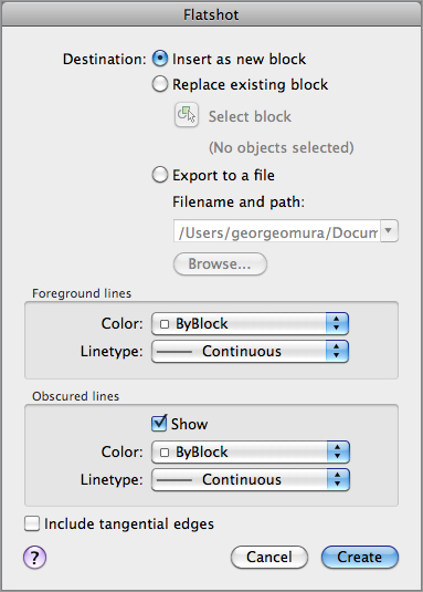
Figure 22-35:The 2D orthogonal views shown in relation to the 3D model

Figure 22-36:You can use a layout to arrange a set of views created by Flatshot. Dimensions, notes, and a title block can be added to complete the layout.

If your model changes and you need to update the orthogonal views, you can repeat the steps listed here. However, instead of selecting Insert As New Block in the Flatshot dialog box, select Replace Existing Block to update the original orthogonal view blocks. If you want, you can include an isometric view to help communicate your design more clearly.
Set Up Standard Views in a Layout Viewport
To set up a layout viewport to display a view, like a top or right-side view of a 3D model, double-click inside the viewport and then select a view from the 3D Views menu on the Viewport Controls. To set the scale of a viewport, click the viewport border (double-click outside the viewport if you cannot select its border) and then select a scale from the VP Scale pop-up menu on the Status Bar palette. If you’d like to refresh your memory on layouts in general, refer to Chapter 15, “Laying Out Your Printer Output.”
Adding Dimensions and Notes in a Layout
Although I don’t recommend adding dimensions in Paper Space for architectural drawings, it may be a good idea for mechanical drawings such as the one in this chapter. By maintaining the dimensions and notes separate from the actual model, you keep these elements from getting in the way of your work on the solid model. You also avoid the confusion of having to scale the text and dimension features properly to ensure that they will plot at the correct size. See Chapter 9, “Adding Text to Drawings,” and Chapter 11, “Using Dimensions,” for a more detailed discussion of notes and dimensions.
As long as you set up your Paper Space work area to be equivalent to the final print size, you can set dimension and text to the sizes you want when you print. If you want text ¼˝ high, you set your text styles to be ¼˝ high.
To include dimensions, make sure you’re in a layout view, and then use the dimension commands in the normal way. However, you need to make sure full associative dimensioning is turned on. Type DIMASSOC↵ 2↵ to turn on associative dimensioning or DIMASSOC↵ 1↵ to turn it off. Dimassoc is the system variable that controls associative dimensioning. With associative dimensioning turned on, dimensions in a layout view display the true dimension of the object being dimensioned, regardless of the scale setting of the viewport.
If you don’t have the associative dimensioning option turned on and your viewports are set to a scale other than 1 to 1, you have another option: You can set the Overall Scale option in the New or Modify Dimension Style dialog box to a proper value. The following steps show you how:
1. Click the Show Drawings & Layouts button in the Status Bar palette, and then select the Model layout for your drawing.
2. Choose Format Dimension Style from the menu bar to open the Dimension Style Manager.
3. Make sure you’ve selected the style you want to edit, and then click the Options action menu and choose Modify to open the Modify Dimension Style dialog box.
4. Click the Primary Units tab.
5. In the Scale Factor input box in the Linear Dimensions group, enter the value by which you want your Paper Space dimensions multiplied. For example, if your Paper Space views are scaled at one-half the actual size of your model, enter 2 in this box to multiply your dimensions’ values by two.
6. Click the Apply To Layout Dimensions Only check box. This ensures that your dimension is scaled only while you’re adding dimensions in Paper Space. Dimensions added in Model Space aren’t affected.
7. Click OK to close the Modify Dimension Style dialog box, and then click Close in the Dimension Style Manager.
You’ve had to complete a lot of steps to get the final drawing, but compared with drawing these views by hand, you undoubtedly saved a great deal of time. In addition, as you’ll see later in this chapter, what you have is more than just a 2D drafted image. With what you created, further refinements are now easy.
Using Visual Styles with a Viewport
In Chapter 19, you saw how you can view your 3D model using visual styles. A visual style can give you a more realistic representation of your 3D model, and it can show off more of the details, especially on rounded surfaces. You can also view and plot a visual style in a layout view. To do this, you make a viewport active and then turn on the visual style you want to use for that viewport. The following exercise gives you a firsthand look at how this is done:
1. Back in the Bracket.dwg drawing, click the Show Drawings & Layouts button in the Status Bar palette and double-click the Layout1 thumbnail.
2. Double-click inside the viewport with the isometric view of the model to switch to Model Space.
3. Select Conceptual from the Visual Styles menu on the Viewport Controls (Figure 22-37).
Figure 22-37:The Visual Styles menu on the Viewport Controls

The view may appear a bit dark because of the black color setting for the object. You can change the color to a lighter one such as cyan or blue to get a better look.
4. Double-click outside the isometric viewport to return to Paper Space.
If you have multiple viewports in a layout, you can change the visual style of one viewport without affecting the other viewports. This can help others visualize your 3D model more clearly.
You’ll also want to know how to control the hard-copy output of a shaded view. For this, you use the shortcut menu:
1. Click the isometric view’s viewport border to select it.
2. Right-click to open the shortcut menu, and select the Shade Plot option to display a set of Shade Plot options (Figure 22-38).
3. Take a moment to study the menu, and then click As Displayed.
Figure 22-38:The Shade Plot submenu

The As Displayed option prints the viewport as it appears in the drawing area. You use this option to print the currently displayed visual style. Wireframe sets the viewport to a Wireframe view. Hidden sets the viewport to a hidden-line view similar to the view you see when you use the Hide command. At the bottom of the menu is the Rendered option, which sets the view to use AutoCAD’s Render feature when printing, described in Chapter 21, “Rendering 3D Drawings.” You can use the Rendered option to print ray-traced renderings of your 3D models.
Remember these options on the shortcut menu as you work on your drawings and when you print. They can be helpful in communicating your ideas, but they can also get lost in the array of tools that AutoCAD offers.
If you’re designing a complex object, sometimes it helps to be able to see it in ways that you couldn’t in the real world. AutoCAD offers two visualization tools that can help others understand your design ideas.
If you want to show off the internal workings of a part or an assembly quickly, you can use the X-ray effect, which can be found in the Visuals Styles menu on the Viewport Controls.
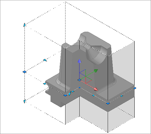
Figure 22-39 shows an isometric view of the bracket using the Vsfaceopacity system variable, which also gives an X-ray-like appearance to your model. The Realistic visual style combined with the Vsfaceopacity system variable gives this effect. The color of the bracket has also been changed to a light gray to help visibility. You can see the internal elements as if the object were semitransparent. The Vsfaceopacity works with any 3D visual style, although it works best with a style that shows some of the surface features (such as the Conceptual or Realistic visual style).
To use it, enter VSFACEOPACITY, and then enter a value for the opacity. You can start with 50 and adjust from there. The default value is –60 for an opaque object.
Figure 22-39:The bracket displayed using a Realistic visual style and the X-ray effect of the Vsfaceopacity command.

Another tool to help you visualize the internal workings of a design is the Sectionplane command. This command creates a plane that defines the location of a cross section. A section plane can also do more than just show a cross section. Try the following exercise to see how it works:
1. In the Bracket file, click Model in the Status Bar palette, select Model from the pop-up menu, and then change the color of layer 0 to a light gray so you can see the bracket more clearly when using the Realistic visual style.
2. Select Realistic from the Visual Styles menu on the Viewport Controls.
3. Make sure that the Object Snap and Object Snap Tracking toggles are turned off in the Status Bar palette. This will allow you to point to surfaces on the model while using the Sectionplane command.
4. Adjust your view so it looks similar to Figure 22-40.
5. Click the Section Plane tool near the bottom of the Tool Sets palette. You can also enter SECTIONPLANE↵ at the Command prompt. You’ll see the following prompt:
Select face or any point to locate
section line or [Draw section/Orthographic]:
6. Click the front plane of the bracket, as shown in Figure 22-40. A plane appears on that surface.
Figure 22-40:Adding the section plane to your bracket

You can move the section plane object along the solid to get a real-time view of the section it traverses. To do this, you need to turn on the Live Section feature. To check whether Live Section is turned on, do the following:
1. Click the section plane, and then right-click. If you see a check mark by the Activate Live Sectioning option, then you know it’s on. If you don’t see a check mark, then choose Activate Live Sectioning to turn it on.
2. Click the red axis on the Move gizmo, as shown in Figure 22-41. The axis turns yellow to indicate that it is active and you see a red vector appear. If you don’t see the gizmo, make sure you are in the Realistic visual style.
Figure 22-41:Moving the surface plane across the bracket
3. Move the cursor slowly toward the back of the bracket.
4. When the section plane is roughly in the middle of the tapered portion of the bracket, click the mouse to fix the plane in place. You should have a view similar to Figure 22-42.
Figure 22-42:The surface plane fixed at a location

Now you see only a portion of the bracket behind the section plane plus the cross section of the plane, as shown in Figure 22-43. You can have the section plane display the front portion as a ghosted image by doing the following:
1. With the section plane selected (you should still see its Move gizmo), right-click and choose Live Section Settings. In the Section Settings dialog box, under the Cut-Away Geometry category, click Show. Click OK. The front portion of the bracket appears in red (Figure 22-43).
2. Press the Esc key to remove the section plane from the current selection. The cut-away geometry remains in view.
Figure 22-43:The front portion of the bracket is displayed with the Show Cut-Away Geometry option turned on.

You can double-click on the section plane to toggle between a solid view and a cut-away view of the geometry. This toggles the Active Live Sectioning option.
You can also add a jog in the section plane to create a more complex section cut. Here’s how it’s done:
1. Select the section plane.
2. Right-click, and choose Add Jog To Section.
3. At the Specify a point on the section line to add jog: prompt, use the Nearest object snap to select a point on the section plane line (Figure 22-44).
Figure 22-44:Moving the jog in the section plane

4. Click the grip on the back portion of the section plane, as shown in Figure 22-44, and drag it toward the right so the jog looks similar to the third panel in the figure.
5. Press the Esc key to get a clear view of the new section.
As you can see from this example, you can adjust the section using the grips on the section plane line. You can use the Nearest osnap to select a point anywhere along the section line to a jog. Click and drag the endpoint grips to rotate the section plane to an angle.
You may have also noticed another arrow in the section plane (Figure 22-45).
Figure 22-45:The arrow presents additional options for the section plane.

When you click the downward-pointing arrow, you see three options for visualizing the section boundary: Section Plane, Section Boundary, and Section Volume.
By using these other settings, you can start to include sections through the sides, back, top, or bottom of the solid. For example, if you click the Section Boundary option, another boundary line appears with grips (Figure 22-46). To see it clearly, you may have to press Esc and then select the section plane again. You can then manipulate these grips to show section cuts along those boundaries.
Figure 22-46:Another boundary line appears with grips when you click the Section Boundary option.

The Section Volume option displays the boundary of a volume along with grips at the top and bottom of the volume (Figure 22-47). These grips allow you to create a cut plane from the top or bottom of the solid.
Figure 22-47:The boundaries shown using the Section Volume option
Finally, you can get a copy of the solid that is behind or in front of the section plane. Right-click the section plane, and choose Generate 2D/3D Section to open the Generate Section/Elevation dialog box. Click the Hide Advanced Settings disclosure triangle to expand the dialog box and display more options (Figure 22-48).
Figure 22-48:The Generate Section/Elevation dialog box

If you select 2D Section/Elevation, a 2D image of the section plane is inserted in the drawing in a manner similar to the insertion of a block. You’re asked for an insertion point, an X and Y scale, and a rotation angle.
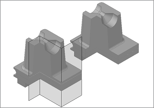
The 3D Section option creates a copy of the portion of the solid that is bounded by the section plane or planes, as shown in Figure 22-49.
Using a Section Plane in an Architectural Model
If your application is architectural, you can use a section plane and the 2D Section/Elevation option to get an accurate elevation drawing. Instead of placing the section plane inside the solid, move it away from the solid model and use the 2D Section/Elevation option.
Figure 22-49:A copy of the solid minus the section area is created using the 3D Section option of the Generate Section/Elevation dialog box.
You can access more detailed settings for the 2D Section/Elevation, 3D Section, and Section Settings options by clicking the Hide Advanced Settings disclosure triangle at the bottom of the Generate Section/Elevation dialog box (Figure 22-50). The Section Settings button near the bottom opens the Section Settings dialog box, which lists the settings for the section feature.
Figure 22-50:The Generate Section/Elevation dialog box
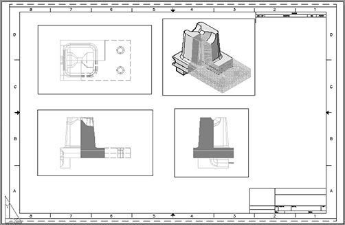
If you create a set of orthogonal views in a layout, the work you do to find a section is also reflected in the layout views (Figure 22-51).
Figure 22-51:A set of orthogonal views in a layout
Taking Advantage of Stereolithography
A discussion of solid modeling wouldn’t be complete without mentioning stereolithography. This is one of the most interesting technological wonders that has appeared as a by-product of 3D computer modeling. Stereolithography is a process that generates physical reproductions of 3D computer solid models. Special equipment converts your AutoCAD-generated files into a physical model.
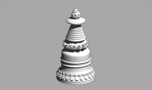
This process offers the mechanical designer a method for rapidly prototyping designs directly from AutoCAD drawings, though applications don’t have to be limited to mechanical design. Architects can take advantage of this process too. My own interest in Tibetan art led me to create a 3D AutoCAD model of a type of statue called a Zola, shown here. I sent this model to a service to have it reproduced in resin.
AutoCAD supports stereolithography through the Export and Stlout commands. These commands generate an STL file, which can be used with a Stereolithograph Apparatus (SLA) to generate a model. You must first create a 3D solid model in AutoCAD. Then you can use the Export Data dialog box to export your drawing in the STL format. Choose File Export from the menu bar, and make sure the File Format pop-up menu shows Lithography (*.stl) before you click the Save button.
The AutoCAD 3D solids are translated into a set of triangular-faceted meshes in the STL file. You can use the Smoothness For 3D Printing/Rendering setting in the Document Settings tab of the Application Preferences dialog box to control the fineness of these meshes. See Chapter 21 for more information on this setting.
Understand solid modeling. Solid modeling lets you build 3D models by creating and joining 3D shapes called solids. There are several built-in solid shapes called primitives, and you can create others using the Extrude tool.
Master It Name some of the built-in solid primitives available in AutoCAD.
Create solid forms. You can use Boolean operations to sculpt 3D solids into the shape you want. Two solids can be joined to form a more complex one, or you can remove one solid from another.
Master It Name the three Boolean operations you can use on solids.
Create complex solids. Besides the primitives, you can create your own shapes based on 2D polylines.
Master It Name three tools that let you convert closed polylines and circles into 3D solids.
Edit solids. Once you’ve created a solid, you can make changes to it using the solid-editing tools offered on the Solids – Edit tool group or the Modify Solid Editing submenu on the menu bar.
Master It Name at least four of the tools found on the Solids – Edit tool group.
Streamline the 2D drawing process. You can create 3D orthogonal views of your 3D model to create standard 2D mechanical drawings.
Master It What is the name of the tool in the Tool Sets palette that lets you create a 2D drawing of a 3D model?
Visualize solids. In addition to viewing your 3D model in a number of different orientations, you can view it as if it were transparent or cut in half.
Master It What is the name of the command that lets you create a cut view of your 3D model?