3.1 Scale and Resolution

The concept of scale underlies all maps. As we know from the discussion of maps in Chapter 2, most maps are graphical representations of the environment that show the world in a smaller format than the reality. The environments and objects that we map are almost always never the same size as the pieces of paper or computer screens that represent them, and scale refers to “the amount of reduction that takes place in going from real-world dimensions to the new mapped area on the map plane” (Dent, Torguson, & Hodler, 2009). This reduction is referred to as map scale, which can be defined as Map Distance/Earth Distance. This equation is generally presented on maps in a ratio format, so the representative fraction 1/24,000 becomes 1:24,000. In this case, the ratio 1:24,000 can be interpreted as one unit of measure on the map representing 24,000 units on the ground.

Maps are often referred to as large-scale or small-scale based on the size of this ratio. The usage of these terms can be confusing. A 1/24,000 scale map shows a smaller surface area with more detail than the 1/1,000,000 scale map, but since the fraction itself is a larger number, it is considered a large-scale map (Foote, 2000). Fig. 3.1 shows an example of how a map of the same area will appear different at different scales.

Scale is central to understanding and interpreting maps. Often map readers are familiar with the area being mapped, and some feature on the map gives context to the scale being represented. In the absence of familiar places or features, the scale declaration on a map is essential to correct interpretation. Fig. 3.2 gives an example of how this functions. Both maps appear visually identical, yet the change in scale leads to a completely different understanding of the pattern that we see.

A concept related to scale is resolution, which comes into play most often in a digital context. Resolution can refer to a few different things, but in a geospatial context it commonly refers to the size in ground units of the pixels found in a raster image.¹ Aerial photography and satellite imagery are commonly described by their spatial resolution, with a higher resolution indicating that each pixel represents a smaller piece of the Earth’s surface.² For example, NASA’s Landsat 8 imaging satellite has multiple sensors that record the Earth’s surface at different resolutions (Garner, 2013). One sensor, the Operational Land Imager, records portions of the electromagnetic radiation spectrum, discussed in Chapter 4, that include visible light at a spatial resolution of 30 m or roughly 100 ft, meaning that each pixel in a Landsat image recorded by this sensor represents 900 m² of surface area. The Thermal Infrared Sensor, a different sensor on the Landsat 8 satellite, has a spatial resolution of 100 m or roughly 330 ft, meaning that each pixel in these images will represent 10,000 m² on the ground. Generally speaking, higher resolutions, meaning smaller pixels, are preferable when it comes to imagery, but it depends on the scale of the features being represented. For example, land cover at the global scale could be represented with 1 km² pixels, while imagery with a resolution of 30 m might be better suited to observing land cover for an individual state. Knowing the resolution of raster imagery is an essential component to correct interpretation.

Resolution can also refer to the precision at which a paper map has been scanned into a digital format. A map that is scanned at 100 dots per inch (dpi) will have a lower resolution than one scanned at 600 dpi. A map scanned at a low resolution will have less detail, much like how a small-scale map will contain less detail than a large-scale map. Fig. 3.3 shows how scanning at different resolutions can affect the quality of the final product.

3.2 Geodesy

Geodesy refers to the study of the size and shape of the Earth (Robinson, Morrison, Muehrcke, Kimerling, & Guptill, 1995, p. 116). Calculating an accurate measurement of the circumference of the Earth has been a challenge to scholars for millennia. The ancient Greek scholar Eratosthenes, who around 240 B.C. used seasonal changes in the sun’s angle to estimate the size of the Earth, came within 15% of today’s precise modern measurements (Brown & Kumar, 2011). Eratosthenes’ circumference assumed that the Earth was spherical, but today we know this is not the case. Rotation along the Earth’s axis causes the poles to be flattened and the Equator to be stretched outward, leading to an ellipsoidal shape. Beyond that, we know today that the surface contains depressions and bumps, which creates a shape described as a geoid. The difference between the three reference shapes can be seen in Fig. 3.4. The differences in these three shapes do not generally affect maps at small scales. Yet, for large-scale maps that require high levels of precision and accuracy, the way the shape of the Earth is defined can be essential.

A datum combines a reference shape, typically an ellipsoid, with a tie point that fixes the reference shape to a position on the Earth. As an example, the North American Datum of 1927 (NAD27) uses the Clarke 1866 ellipsoid and puts its tie point at Meades Ranch, Kansas, Untied States, 39°13′26.68″N, 98°32′30.51″W, see Fig. 3.5. This provides the map creator with a surface to work with and a point of reference from which to start. The updated North American Datum of 1983 (NAD83) uses the Geodetic Reference System 1980 (GRS80) ellipsoid, and uses the center of the Earth as its tie point. In a digital GIS context, it is important to select the correct datum for the data used, as an incorrect datum can lead to reduced locational accuracy in the data, particularly on large-scale maps. This can lead to misalignment when multiple datasets are viewed simultaneously and errors in analysis output.

3.3 Projections

Maps are two-dimensional representations of three-dimensional space. Typically, they show a portion of the Earth’s surface, and as we have seen, the surface is rarely, if ever, flat. Projections are the tools that cartographers use to take the curved surface of the Earth and transform it to a two-dimensional map representation. Much like peeling an orange, the curved surface of the Earth cannot be made flat without distorting it in one way or another. Different projections have different approaches to how they mathematically transform earth-surface geometry to map geometry, but all projections create distortion in one or more geometric measures.

Projections begin with a datum, which is the combination of reference surface and tie point; then, an appropriate geometric developable surface is chosen. Developable surfaces are the “flat” surfaces that maps are projected onto, and can be planes, cylinders, or cones. These surfaces also have the option of being either tangent or secant to the surface of the earth. On a tangent surface, the developable plane touches the Earth once, at either a standard point or standard line. In the secant case, the developable surface cuts through the Earth and creates either one or two standard lines. These standard points and lines are important, as they represent the portions of the map with the least amount of distortion. The further away on the map from a standard point or lines one gets, the more geometric distortion exists. A visual example of the three types of geometric developable surfaces and their standard points/lines can be seen in Fig. 3.6.

Purely mathematical projections not based on a geometric developable surface are also possible. Some resemble the geometric forms and are referred to as pseudocylindrical, pseudoconic, and pseudoazimuthal. The Mollweide projection is a pseudocylindrical projection, which can be seen in Fig. 3.7.

Next, the geometric properties of a projection must be considered. Equal-area projections, also known as equivalent projections, ensure that surface area is correctly preserved following transformation, but often at the expense of preserving correct shapes. The Hammer-Aitoff projection is an example of an equal-area projection, seen in Fig. 3.8A.

Conformal projections, known as orthomorphic projections, preserve the shapes of small areas around standard points or lines, while larger shapes such as continents may be highly distorted. The Mercator projection is an example of a conformal projection. Shapes are preserved close to a standard line on the Equator, but become more distorted farther away as seen in Fig. 3.8B.

Equidistant projections preserve distances of great circles, which are lines that converge at the poles. Distances in these projections are true from one or a few standard points to all other points, but they are not true between all points to all other points. Azimuthal projections can be equidistant and show true directions from a central point to all other points. Directions from noncentral points will not be accurate. Azimuthal approaches are not exclusive and can coexist with equivalent, conformal, and equidistant on the same map, although not all at once. An example of the South Pole Lambert Azimuthal Equal Area projection can be seen in Fig. 3.8C.

An attempt to find a good balance between the approaches can be found in minimum error or compromise projections that attempt to minimize error in all geometric factors. Error will exist in terms of shape, area, distance, and directions, but they are made to be as small as possible. These projections can be useful when a map does not need to have any one specific property preserved and does not wish to have the large distortions that can occur with other approaches. A compromise example can be seen in the Robinson projection in Fig. 3.8D.

The choice of a “correct” projection depends entirely on the goals of the map. If visual appearance is important, a compromise approach may be desirable, as it does not distort the map much in any measure. However, if a map is to be used for a specific purpose, the correct projection makes all the difference. For navigation, the preserved angles and compass bearings of the Mercator projection would be quite useful. Likewise, if measuring surface area was the purpose of a map, an equivalent projection would be called for. Many projections are used beyond this brief introduction, but it is important to remember that there is no one “correct” projection, only a toolbox of different projections that are appropriate for different circumstances.

3.4 North Defined

One convention of mapmaking is that the top edge of the map points northward, although this is not always true particularly for older maps. This makes map interpretation easier, as readers are not required to reorient their mental orientation. North arrows are an essential component of maps, especially for maps where north is not at the top of the page. To assume the north arrow will always point up is an over-simplification though. For one, on small-scale maps, north may not be a consistent direction on the page. A single north arrow may point toward the top of the page, but this is not always accurate, as can be seen in Fig. 3.9.

Also, differences exist between the locations of geographic north and magnetic north. Geographic north represents the place where the Earth’s axis of rotation exists. Magnetic north represents the location near geographic north where the Earth’s magnetic field points vertically downward. The difference between the two is called magnetic declination, and the difference changes depending on both the location of a map and when the map is set, as the Earth’s magnetic field is constantly shifting. USGS topographic maps will include the magnetic declination for each quadrangle. Knowing the magnetic declination of a place is essential to navigation via compass, particularly as one travels longer distances via compass bearing.

Fig. 3.10 shows an example of a statement of magnetic declination on a USGS topographic map. An excellent online resource shows past and present magnetic declination for any place in the world, displayed on the National Geophysical Data Center’s, Historical Declination Viewer (National Oceanic and Atmospheric Administration, 2015).

3.5 Legends

Cartographers use visual symbols to represent features on a map, and legends exist as a way to decode these markers. Some symbols may be labeled or otherwise self-evident on the page, but a mapmaker cannot assume that all readers will be familiar with the visual shorthand employed, and legends exist to explain what all the symbols on the page mean.³ For general reference maps, these might be dots, squares, triangles, or stars that might represent different human-built features on the landscape. For thematic maps that display a distribution of a variable, or the results of an analysis, the legend allows the reader to interpret the different colors, shading, or size of symbols on the page. Legends may also include ancillary information regarding data distributions or methods for maps that involve statistical analyses. One common way that information in a legend can be useful is describing how maps symbolize terrain, as described in Chapter 2.

3.6 Grids and Graticules

In order to keep track of the location of places and objects on the Earth, grids are often employed. These grids, or coordinate systems, are at their most basic no more complicated than simple Cartesian planes, with a starting origin and X, Y measurements to represent a location within the grid. The grid will have uniformly spaced lines with intersections having right angles without regard to the curvature of Earth (Larsgaard, 1998, p. 261).

Some coordinate systems use +/− notation to indicate locations in relation to the origin. Other coordinate systems apply a false origin, arbitrary numbers added to the coordinates, to ensure that no coordinate numbers will ever be negative within the system. It is coordinate systems, along with a datum that gives reference to the surface, that allow us to make the geometric transformations necessary for projections.

Although similar in appearance, the graticule is not equivalent to a coordinate system. Rather, graticules are spherical indicators of the imaginary network of parallels and meridians representing latitude and longitude on a map. While useful as a reference to location, a graticule cannot be used for computational purposes in the same way that coordinate systems can (Iliffe, 2000). Examples of graticules can be seen in Figs. 3.8 and 3.9.

As an example of grids and graticules, many map librarians may be familiar with historic USGS large-scale topographic quadrangles that show one graticule and two grids. Again, the graticule is the latitude/longitude system; whereas, grids are Universal Transverse Mercator (UTM) and U.S. Public Land Survey System.

3.7 Latitude and Longitude

One of the most commonly used methods of referencing locations on the Earth is the latitude and longitude system. Latitude is the angular measure of a location north or south of the Equator. It can be easily measured using the angle above the horizon of either the Sun or a Pole Star. In the northern hemisphere and near the Equator, Polaris, known as the North Star, is the pole star. In the southern hemisphere, the pole star is the faint South Star or Sigma Octantis, but navigators have long relied upon two stars in the Southern Cross constellation that point in the direction of the South Pole. The fact that we are measuring in angles is a hint that latitude and longitude are measures of a spherical Earth, whereas the coordinate systems described later in this chapter are two-dimensional representations. While the measurement of latitude has a straightforward physical basis in the Equator, longitude is based on an arbitrary starting point known as the Prime Meridian located in Greenwich, England. Historically several prime meridians were in use by different countries, but the current accepted Prime Meridian is the one in Greenwich, see Fig. 3.11.

Longitude was a more challenging measurement in historic times, with a reliable solution not appearing until John Harrison’s Marine Chronometer was invented in the 18th century. Harrison’s sea-worthy timepiece was an answer to the British Board of Longitude’s challenge, for which he received the Longitude Prize, a considerable cash sum of more than £15,000 (Brown, 1949). Today, latitude and longitude are most commonly measured using global positioning systems (GPS) such as the U.S.’s NAVSTAR system or Russia’s GLONASS system.

Lines of latitude are referred to as parallels, as the surface distance of one degree is always a consistent 111 km. Lines of longitude are referred to as meridians, and the distances from one to the next are 111 km at the Equator, but become shorter as they approach the poles where the meridians converge. Measures of latitude/longitude can be notated as either degrees-minutes-seconds (DMS) or decimal degrees (DD) and can use either a cardinal direction or +/− symbols to indicate direction from the Equator or Prime Meridian, as seen in Table 3.1.

3.8 Universal Transverse Mercator Coordinate System

The Universal Transverse Mercator (UTM) system was created by several allied nations following World War II (Dracup, 2006a). This system was an attempt to have a unified, projected two-dimensional coordinate system as opposed to sharing information between nations in multiple disparate formats. The system covers from 80°S to 84°N, and divides the Earth into 60 six-degree sections east-west. It uses a secant Transverse Mercator projection with a base unit of the meter, and is accurate to one part in 2500. UTM is commonly used in a GIS context, as it covers, and is consistent, across most of the Earth’s surface. The Polar Regions not covered by the UTM system are covered by the Universal Polar Stereographic System.

3.9 State Plane Coordinate System

The State Plane Coordinate System (SPCS or SPC) was created in the 1930s in the United States as a way to allow engineers and others to work within a system of two-dimensional plane geometry as opposed to having to use more complex spherical calculations (Dracup, 2006b). Accuracies are one part in 10,000, as the different SPC zones are small enough that they can reduce geometric distortion more so than the larger zones found in the UTM system.

The original SPC system relied on the NAD27 datum and the foot as a unit of measure, but today SPC uses the NAD83 datum, and the meter as the unit of measure. Some states have only one SPC zone, but many have two or more zones of coverage. SPC zones that are elongated east-west use a secant Lambert Conformal Conic projection, while north-south elongated zones use a secant Transverse Mercator projection. A secant Oblique Mercator projection is used for one section in Alaska. Zones use a false origin to ensure that all coordinates within the zone will be positive values, the exact specifics depending on the zone in question.

3.10 Public Land Survey System

In the United States, the Public Land Survey System (PLSS) is one the of the most important grid systems in use for managing land ownership and infrastructure. It differs from UTM and SPC in that its basic unit is the acre, and it is defined from the ground, not from a virtual grid (Robinson et al., 1995). It establishes a series of origins, known as principal meridians and base lines, from which further measurements are based. These origins are visible in Fig. 3.12.

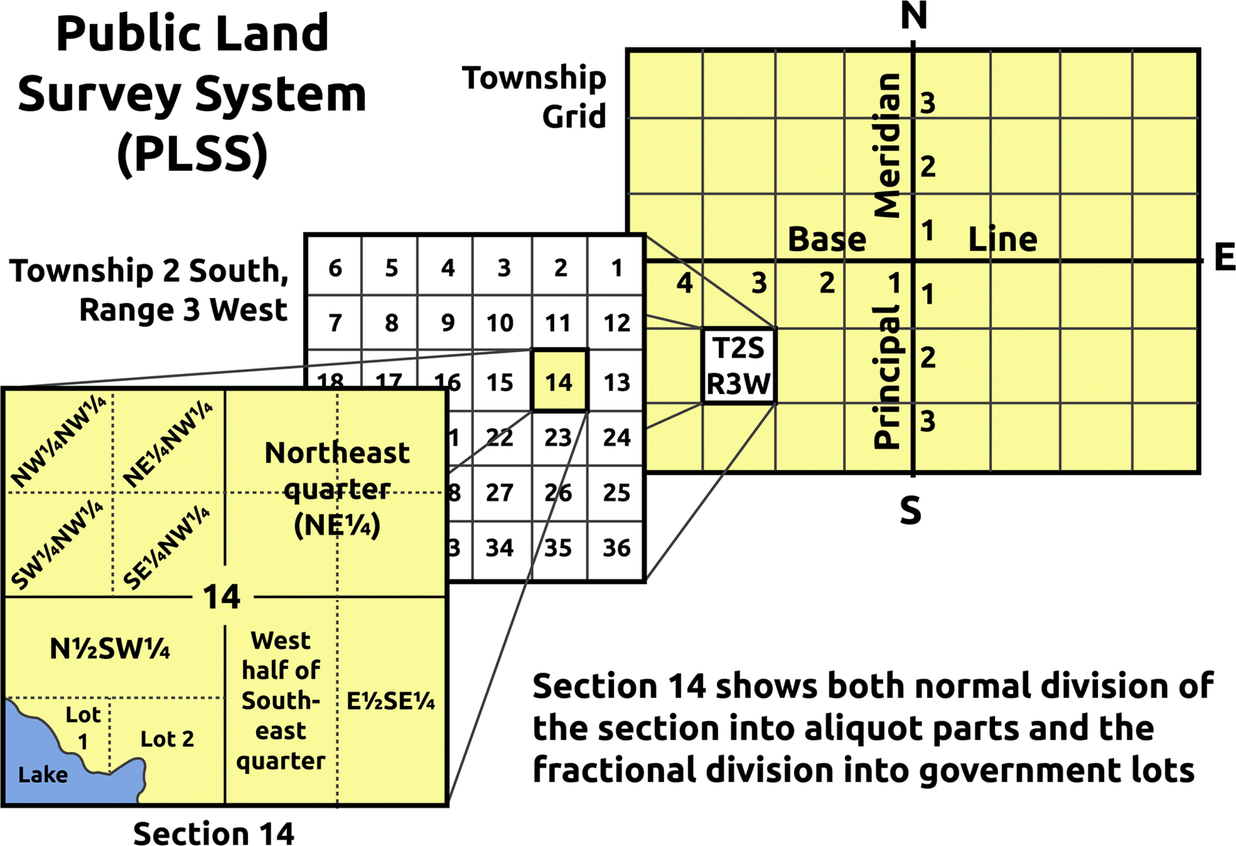
In the PLSS, land is partitioned into six-mile squares, identified by a township number N/S of the base line, and a range number E/W of the principal meridian. These six-mile squares are further divided into 36 sq mi sections. Each of these 36 sections may be subdivided into quarters, which can be further subdivided into quarter-quarters. A subsection’s location might be described as the northeast quarter of the northwest quarter of section 4, township 18 south, range 9 east, Sixth meridian, Kansas. The layout of township and range can be seen in Fig. 3.13.

While the PLSS dominates the landscape of most states west of the Appalachian Mountains in the United States, an older system of land surveying can be found in the metes and bounds system. The system is interpreted as measure of the limits of a boundary. This system describes land parcels by beginning with a landmark as an origin and giving a verbal description of the boundaries “walking” around the edges. This survey system does not adhere to any grid, and therefore tends to describe more irregular shapes than the neat, rectilinear layout of the PLSS.

There are 19 Eastern states settled before the Land Ordinance of 1785 and Northwest Ordinance of 1787, which were the beginnings of the PLSS (U.S. Geological Survey, 2016). The survey system used in Hawaii is Kingdom of Hawaii native system and in the others, the British system of metes and bounds or some combination of PLSS with the British system or Spanish and French Land Grants. Legal land descriptions regardless of the system are used for identifying ownership and taxation. It can be confusing integrating the methods used in different states and countries and adjusting for the three-dimensional Earth, represented in a two-dimensional plane of a map.

3.11 Conclusions

Cartography is a complex subject, marrying the visual graphic arts and the sciences of data visualization and Earth measurement in equal parts to create coherent, informative maps. Today, our digital culture is adding factors of location tracking and navigation through global positioning systems, real-time map modification, and interactive maps to the toolbox. Despite these changes in the field of cartography, the underlying structure of maps remains similar to that of the maps created in antiquity. Understanding some of the basic concepts used to create maps will allow librarians and library users to better interpret and use them, as well as find maps that serve their specific needs.