Chapter 3. Understanding TensorFlow Basics
This chapter demonstrates the key concepts of how TensorFlow is built and how it works with simple and intuitive examples. You will get acquainted with the basics of TensorFlow as a numerical computation library using dataflow graphs. More specifically, you will learn how to manage and create a graph, and be introduced to TensorFlow’s “building blocks,” such as constants, placeholders, and Variables.
Computation Graphs
TensorFlow allows us to implement machine learning algorithms by creating and computing operations that interact with one another. These interactions form what we call a “computation graph,” with which we can intuitively represent complicated functional architectures.
What Is a Computation Graph?
We assume a lot of readers have already come across the mathematical concept of a graph. For those to whom this concept is new, a graph refers to a set of interconnected entities, commonly called nodes or vertices. These nodes are connected to each other via edges. In a dataflow graph, the edges allow data to “flow” from one node to another in a directed manner.
In TensorFlow, each of the graph’s nodes represents an operation, possibly applied to some input, and can generate an output that is passed on to other nodes. By analogy, we can think of the graph computation as an assembly line where each machine (node) either gets or creates its raw material (input), processes it, and then passes the output to other machines in an orderly fashion, producing subcomponents and eventually a final product when the assembly process comes to an end.
Operations in the graph include all kinds of functions, from simple arithmetic ones such as subtraction and multiplication to more complex ones, as we will see later on. They also include more general operations like the creation of summaries, generating constant values, and more.
The Benefits of Graph Computations
TensorFlow optimizes its computations based on the graph’s connectivity. Each graph has its own set of node dependencies. When the input of node y is affected by the output of node x, we say that node y is dependent on node x. We call it a direct dependency when the two are connected via an edge, and an indirect dependency otherwise. For example, in Figure 3-1 (A), node e is directly dependent on node c, indirectly dependent on node a, and independent of node d.

Figure 3-1. (A) Illustration of graph dependencies. (B) Computing node e results in the minimal amount of computations according to the graph’s dependencies—in this case computing only nodes c, b, and a.
We can always identify the full set of dependencies for each node in the graph. This is a fundamental characteristic of the graph-based computation format. Being able to locate dependencies between units of our model allows us to both distribute computations across available resources and avoid performing redundant computations of irrelevant subsets, resulting in a faster and more efficient way of computing things.
Graphs, Sessions, and Fetches
Roughly speaking, working with TensorFlow involves two main phases: (1) constructing a graph and (2) executing it. Let’s jump into our first example and create something very basic.
Creating a Graph
Right after we import TensorFlow (with import tensorflow as tf), a specific empty default graph is formed. All the nodes we create are automatically associated with that default graph.
Using the tf.<operator> methods, we will create six nodes assigned to arbitrarily named variables. The contents of these variables should be regarded as the output of the operations, and not the operations themselves. For now we refer to both the operations and their outputs with the names of their corresponding variables.
The first three nodes are each told to output a constant value. The values 5, 2, and 3 are assigned to a, b, and c, respectively:
a=tf.constant(5)b=tf.constant(2)c=tf.constant(3)
Each of the next three nodes gets two existing variables as inputs, and performs simple arithmetic operations on them:
d=tf.multiply(a,b)e=tf.add(c,b)f=tf.subtract(d,e)
Node d multiplies the outputs of nodes a and b. Node e adds the outputs of nodes b and c. Node f subtracts the output of node e from that of node d.
And voilà! We have our first TensorFlow graph! Figure 3-2 shows an illustration of the graph we’ve just created.

Figure 3-2. An illustration of our first constructed graph. Each node, denoted by a lowercase letter, performs the operation indicated above it: Const for creating constants and Add, Mul, and Sub for addition, multiplication, and subtraction, respectively. The integer next to each edge is the output of the corresponding node’s operation.
Note that for some arithmetic and logical operations it is possible to use operation shortcuts instead of having to apply tf.<operator>. For example, in this graph we could have used */+/- instead of tf.multiply()/tf.add()/tf.subtract() (like we did in the “hello world” example in Chapter 2, where we used + instead of tf.add()). Table 3-1 lists the available shortcuts.
| TensorFlow operator | Shortcut | Description |
|---|---|---|
tf.add() |
a + b |
Adds a and b, element-wise. |
tf.multiply() |
a * b |
Multiplies a and b, element-wise. |
tf.subtract() |
a - b |
Subtracts b from a, element-wise. |
tf.divide() |
a / b |
Computes Python-style division of a by b. |
tf.pow() |
a ** b |
Returns the result of raising each element in a to its corresponding element b, element-wise. |
tf.mod() |
a % b |
Returns the element-wise modulo. |
tf.logical_and() |
a & b |
Returns the truth table of a & b, element-wise. dtype must be tf.bool. |
tf.greater() |
a > b |
Returns the truth table of a > b, element-wise. |
tf.greater_equal() |
a >= b |
Returns the truth table of a >= b, element-wise. |
tf.less_equal() |
a <= b |
Returns the truth table of a <= b, element-wise. |
tf.less() |
a < b |
Returns the truth table of a < b, element-wise. |
tf.negative() |
-a |
Returns the negative value of each element in a. |
tf.logical_not() |
~a |
Returns the logical NOT of each element in a. Only compatible with Tensor objects with dtype of tf.bool. |
tf.abs() |
abs(a) |
Returns the absolute value of each element in a. |
tf.logical_or() |
a | b |
Returns the truth table of a | b, element-wise. dtype must be tf.bool. |
Creating a Session and Running It
Once we are done describing the computation graph, we are ready to run the computations that it represents. For this to happen, we need to create and run a session. We do this by adding the following code:
sess=tf.Session()outs=sess.run(f)sess.close()("outs = {}".format(outs))Out:outs=5
First, we launch the graph in a tf.Session. A Session object is the part of the TensorFlow API that communicates between Python objects and data on our end, and the actual computational system where memory is allocated for the objects we define, intermediate variables are stored, and finally results are fetched for us.
sess=tf.Session()
The execution itself is then done with the .run() method of the Session object. When called, this method completes one set of computations in our graph in the following manner: it starts at the requested output(s) and then works backward, computing nodes that must be executed according to the set of dependencies. Therefore, the part of the graph that will be computed depends on our output query.
In our example, we requested that node f be computed and got its value, 5, as output:
outs=sess.run(f)
When our computation task is completed, it is good practice to close the session using the sess.close() command, making sure the resources used by our session are freed up. This is an important practice to maintain even though we are not obligated to do so for things to work:
sess.close()
Example 3-1. Try it yourself! Figure 3-3 shows another two graph examples. See if you can produce these graphs yourself.

Figure 3-3. Can you create graphs A and B? (To produce the sine function, use tf.sin(x)).
Constructing and Managing Our Graph
As mentioned, as soon as we import TensorFlow, a default graph is automatically created for us. We can create additional graphs and control their association with some given operations. tf.Graph() creates a new graph, represented as a TensorFlow object. In this example we create another graph and assign it to the variable g:
importtensorflowastf(tf.get_default_graph())g=tf.Graph()(g)Out:<tensorflow.python.framework.ops.Graphobjectat0x7fd88c3c07d0><tensorflow.python.framework.ops.Graphobjectat0x7fd88c3c03d0>
At this point we have two graphs: the default graph and the empty graph in g. Both are revealed as TensorFlow objects when printed. Since g hasn’t been assigned as the default graph, any operation we create will not be associated with it, but rather with the default one.
We can check which graph is currently set as the default by using tf.get_default_graph(). Also, for a given node, we can view the graph it’s associated with by using the <node>.graph attribute:
g=tf.Graph()a=tf.constant(5)(a.graphisg)(a.graphistf.get_default_graph())Out:FalseTrue
In this code example we see that the operation we’ve created is associated with the default graph and not with the graph in g.
To make sure our constructed nodes are associated with the right graph we can construct them using a very useful Python construct: the with statement.
The with statement
The with statement is used to wrap the execution of a block with methods defined by a context manager—an object that has the special method functions .__enter__() to set up a block of code and .__exit__() to exit the block.
In layman’s terms, it’s very convenient in many cases to execute some code that requires “setting up” of some kind (like opening a file, SQL table, etc.) and then always “tearing it down” at the end, regardless of whether the code ran well or raised any kind of exception. In our case we use with to set up a graph and make sure every piece of code will be performed in the context of that graph.
We use the with statement together with the as_default() command, which returns a context manager that makes this graph the default one. This comes in handy when working with multiple graphs:
g1=tf.get_default_graph()g2=tf.Graph()(g1istf.get_default_graph())withg2.as_default():(g1istf.get_default_graph())(g1istf.get_default_graph())Out:TrueFalseTrue
The with statement can also be used to start a session without having to explicitly close it. This convenient trick will be used in the following examples.
Fetches
In our initial graph example, we request one specific node (node f) by passing the variable it was assigned to as an argument to the sess.run() method. This argument is called fetches, corresponding to the elements of the graph we wish to compute. We can also ask sess.run() for multiple nodes’ outputs simply by inputting a list of requested nodes:
withtf.Session()assess:fetches=[a,b,c,d,e,f]outs=sess.run(fetches)("outs = {}".format(outs))(type(outs[0]))Out:outs=[5,2,3,10,5,5]<type'numpy.int32'>
We get back a list containing the outputs of the nodes according to how they were ordered in the input list. The data in each item of the list is of type NumPy.
NumPy
NumPy is a popular and useful Python package for numerical computing that offers many functionalities related to working with arrays. We assume some basic familiarity with this package, and it will not be covered in this book. TensorFlow and NumPy are tightly coupled—for example, the output returned by sess.run() is a NumPy array. In addition, many of TensorFlow’s operations share the same syntax as functions in NumPy. To learn more about NumPy, we refer the reader to Eli Bressert’s book SciPy and NumPy (O’Reilly).
We mentioned that TensorFlow computes only the essential nodes according to the set of dependencies. This is also manifested in our example: when we ask for the output of node d, only the outputs of nodes a and b are computed. Another example is shown in Figure 3-1(B). This is a great advantage of TensorFlow—it doesn’t matter how big and complicated our graph is as a whole, since we can run just a small portion of it as needed.
Automatically closing the session
Opening a session using the with clause will ensure the session is automatically closed once all computations are done.
Flowing Tensors
In this section we will get a better understanding of how nodes and edges are actually represented in TensorFlow, and how we can control their characteristics. To demonstrate how they work, we will focus on source operations, which are used to initialize values.
Nodes Are Operations, Edges Are Tensor Objects
When we construct a node in the graph, like we did with tf.add(), we are actually creating an operation instance. These operations do not produce actual values until the graph is executed, but rather reference their to-be-computed result as a handle that can be passed on—flow—to another node. These handles, which we can think of as the edges in our graph, are referred to as Tensor objects, and this is where the name TensorFlow originates from.
TensorFlow is designed such that first a skeleton graph is created with all of its components. At this point no actual data flows in it and no computations take place. It is only upon execution, when we run the session, that data enters the graph and computations occur (as illustrated in Figure 3-4). This way, computations can be much more efficient, taking the entire graph structure into consideration.

Figure 3-4. Illustrations of before (A) and after (B) running a session. When the session is run, actual data “flows” through the graph.
In the previous section’s example, tf.constant() created a node with the corresponding passed value. Printing the output of the constructor, we see that it’s actually a Tensor object instance. These objects have methods and attributes that control their behavior and that can be defined upon creation.
In this example, the variable c stores a Tensor object with the name Const_52:0, designated to contain a 32-bit floating-point scalar:
c=tf.constant(4.0)(c)Out:Tensor("Const_52:0",shape=(),dtype=float32)
A note on constructors
The tf.<operator> function could be thought of as a constructor, but to be more precise, this is actually not a constructor at all, but rather a factory method that sometimes does quite a bit more than just creating the operator objects.
Setting attributes with source operations
Each Tensor object in TensorFlow has attributes such as name, shape, and dtype that help identify and set the characteristics of that object. These attributes are optional when creating a node, and are set automatically by TensorFlow when missing. In the next section we will take a look at these attributes. We will do so by looking at Tensor objects created by ops known as source operations. Source operations are operations that create data, usually without using any previously processed inputs. With these operations we can create scalars, as we already encountered with the tf.constant() method, as well as arrays and other types of data.
Data Types
The basic units of data that pass through a graph are numerical, Boolean, or string elements. When we print out the Tensor object c from our last code example, we see that its data type is a floating-point number. Since we didn’t specify the type of data, TensorFlow inferred it automatically. For example 5 is regarded as an integer, while anything with a decimal point, like 5.1, is regarded as a floating-point number.
We can explicitly choose what data type we want to work with by specifying it when we create the Tensor object. We can see what type of data was set for a given Tensor object by using the attribute dtype:
c=tf.constant(4.0,dtype=tf.float64)(c)(c.dtype)Out:Tensor("Const_10:0",shape=(),dtype=float64)<dtype:'float64'>
Explicitly asking for (appropriately sized) integers is on the one hand more memory conserving, but on the other may result in reduced accuracy as a consequence of not tracking digits after the decimal point.
Casting
It is important to make sure our data types match throughout the graph—performing an operation with two nonmatching data types will result in an exception. To change the data type setting of a Tensor object, we can use the tf.cast() operation, passing the relevant Tensor and the new data type of interest as the first and second arguments, respectively:
x=tf.constant([1,2,3],name='x',dtype=tf.float32)(x.dtype)x=tf.cast(x,tf.int64)(x.dtype)Out:<dtype:'float32'><dtype:'int64'>
TensorFlow supports many data types. These are listed in Table 3-2.
| Data type | Python type | Description |
|---|---|---|
DT_FLOAT |
tf.float32 |
32-bit floating point. |
DT_DOUBLE |
tf.float64 |
64-bit floating point. |
DT_INT8 |
tf.int8 |
8-bit signed integer. |
DT_INT16 |
tf.int16 |
16-bit signed integer. |
DT_INT32 |
tf.int32 |
32-bit signed integer. |
DT_INT64 |
tf.int64 |
64-bit signed integer. |
DT_UINT8 |
tf.uint8 |
8-bit unsigned integer. |
DT_UINT16 |
tf.uint16 |
16-bit unsigned integer. |
DT_STRING |
tf.string |
Variable-length byte array. Each element of a Tensor is a byte array. |
DT_BOOL |
tf.bool |
Boolean. |
DT_COMPLEX64 |
tf.complex64 |
Complex number made of two 32-bit floating points: real and imaginary parts. |
DT_COMPLEX128 |
tf.complex128 |
Complex number made of two 64-bit floating points: real and imaginary parts. |
DT_QINT8 |
tf.qint8 |
8-bit signed integer used in quantized ops. |
DT_QINT32 |
tf.qint32 |
32-bit signed integer used in quantized ops. |
DT_QUINT8 |
tf.quint8 |
8-bit unsigned integer used in quantized ops. |
Tensor Arrays and Shapes
A source of potential confusion is that two different things are referred to by the name, Tensor. As used in the previous sections, Tensor is the name of an object used in the Python API as a handle for the result of an operation in the graph. However, tensor is also a mathematical term for n-dimensional arrays. For example, a 1×1 tensor is a scalar, a 1×n tensor is a vector, an n×n tensor is a matrix, and an n×n×n tensor is just a three-dimensional array. This, of course, generalizes to any dimension. TensorFlow regards all the data units that flow in the graph as tensors, whether they are multidimensional arrays, vectors, matrices, or scalars. The TensorFlow objects called Tensors are named after these mathematical tensors.
To clarify the distinction between the two, from now on we will refer to the former as Tensors with a capital T and the latter as tensors with a lowercase t.
As with dtype, unless stated explicitly, TensorFlow automatically infers the shape of the data. When we printed out the Tensor object at the beginning of this section, it showed that its shape was (), corresponding to the shape of a scalar.
Using scalars is good for demonstration purposes, but most of the time it’s much more practical to work with multidimensional arrays. To initialize high-dimensional arrays, we can use Python lists or NumPy arrays as inputs. In the following example, we use as inputs a 2×3 matrix using a Python list and then a 3D NumPy array of size 2×3×4 (two matrices of size 3×4):
importnumpyasnpc=tf.constant([[1,2,3],[4,5,6]])("Python List input: {}".format(c.get_shape()))c=tf.constant(np.array([[[1,2,3,4],[5,6,7,8],[9,8,7,6]],[[1,1,1,1],[2,2,2,2],[3,3,3,3]]]))("3d NumPy array input: {}".format(c.get_shape()))Out:Pythonlistinput:(2,3)3dNumPyarrayinput:(2,3,4)
The get_shape() method returns the shape of the tensor as a tuple of integers. The number of integers corresponds to the number of dimensions of the tensor, and each integer is the number of array entries along that dimension. For example, a shape of (2,3) indicates a matrix, since it has two integers, and the size of the matrix is 2×3.
Other types of source operation constructors are very useful for initializing constants in TensorFlow, like filling a constant value, generating random numbers, and creating sequences.
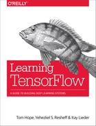
Random-number generators have special importance as they are used in many cases to create the initial values for TensorFlow Variables, which will be introduced shortly. For example, we can generate random numbers from a normal distribution using tf.random.normal(), passing the shape, mean, and standard deviation as the first, second, and third arguments, respectively. Another two examples for useful random initializers are the truncated normal that, as its name implies, cuts off all values below and above two standard deviations from the mean, and the uniform initializer that samples values uniformly within some interval [a,b).
Examples of sampled values for each of these methods are shown in Figure 3-5.

Figure 3-5. 50,000 random samples generated from (A) standard normal distribution, (B) truncated normal, and (C) uniform [–2,2).
Those who are familiar with NumPy will recognize some of the initializers, as they share the same syntax. One example is the sequence generator tf.linspace(a, b, n) that creates n evenly spaced values from a to b.
A feature that is convenient to use when we want to explore the data content of an object is tf.InteractiveSession(). Using it and the .eval() method, we can get a full look at the values without the need to constantly refer to the session object:
sess=tf.InteractiveSession()c=tf.linspace(0.0,4.0,5)("The content of 'c':{}".format(c.eval()))sess.close()Out:Thecontentof'c':[0.1.2.3.4.]
Interactive sessions
tf.InteractiveSession() allows you to replace the usual tf.Session(), so that you don’t need a variable holding the session for running ops. This can be useful in interactive Python environments, like when writing IPython notebooks, for instance.
We’ve mentioned only a few of the available source operations. Table 3-2 provides short descriptions of more useful initializers.
| TensorFlow operation | Description |
|---|---|
tf.constant(value) |
Creates a tensor populated with the value or values specified by the argument |
tf.fill(shape, value) |
Creates a tensor of shape shape and fills it with value |
tf.zeros(shape) |
Returns a tensor of shape shape with all elements set to 0 |
tf.zeros_like(tensor) |
Returns a tensor of the same type and shape as tensor with all elements set to 0 |
tf.ones(shape) |
Returns a tensor of shape shape with all elements set to 1 |
tf.ones_like(tensor) |
Returns a tensor of the same type and shape as tensor with all elements set to 1 |
tf.random_normal(shape, mean, stddev) |
Outputs random values from a normal distribution |
tf.truncated_normal(shape, mean, stddev) |
Outputs random values from a truncated normal distribution (values whose magnitude is more than two standard deviations from the mean are dropped and re-picked) |
tf.random_uniform(shape, minval, maxval) |
Generates values from a uniform distribution in the range [minval, maxval) |
tf.random_shuffle(tensor) |
Randomly shuffles a tensor along its first dimension |
Matrix multiplication
This very useful arithmetic operation is performed in TensorFlow via the tf.matmul(A,B) function for two Tensor objects A and B.
Say we have a Tensor storing a matrix A and another storing a vector x, and we wish to compute the matrix product of the two:
Ax = b
Before using matmul(), we need to make sure both have the same number of dimensions and that they are aligned correctly with respect to the intended multiplication.
In the following example, a matrix A and a vector x are created:
A=tf.constant([[1,2,3],[4,5,6]])(A.get_shape())x=tf.constant([1,0,1])(x.get_shape())Out:(2,3)(3,)
In order to multiply them, we need to add a dimension to x, transforming it from a 1D vector to a 2D single-column matrix.
We can add another dimension by passing the Tensor to tf.expand_dims(), together with the position of the added dimension as the second argument. By adding another dimension in the second position (index 1), we get the desired outcome:
x=tf.expand_dims(x,1)(x.get_shape())b=tf.matmul(A,x)sess=tf.InteractiveSession()('matmul result:{}'.format(b.eval()))sess.close()Out:(3,1)matmulresult:[[4][10]]
If we want to flip an array, for example turning a column vector into a row vector or vice versa, we can use the tf.transpose() function.
Names
Each Tensor object also has an identifying name. This name is an intrinsic string name, not to be confused with the name of the variable. As with dtype, we can use the .name attribute to see the name of the object:
withtf.Graph().as_default():c1=tf.constant(4,dtype=tf.float64,name='c')c2=tf.constant(4,dtype=tf.int32,name='c')(c1.name)(c2.name)Out:c:0c_1:0
The name of the Tensor object is simply the name of its corresponding operation (“c”; concatenated with a colon), followed by the index of that tensor in the outputs of the operation that produced it—it is possible to have more than one.
Duplicate names
Objects residing within the same graph cannot have the same name—TensorFlow forbids it. As a consequence, it will automatically add an underscore and a number to distinguish the two. Of course, both objects can have the same name when they are associated with different graphs.
Name scopes
Sometimes when dealing with a large, complicated graph, we would like to create some node grouping to make it easier to follow and manage. For that we can hierarchically group nodes together by name. We do so by using tf.name_scope("prefix") together with the useful with clause again:
withtf.Graph().as_default():c1=tf.constant(4,dtype=tf.float64,name='c')withtf.name_scope("prefix_name"):c2=tf.constant(4,dtype=tf.int32,name='c')c3=tf.constant(4,dtype=tf.float64,name='c')(c1.name)(c2.name)(c3.name)Out:c:0prefix_name/c:0prefix_name/c_1:0
In this example we’ve grouped objects contained in variables c2 and c3 under the scope prefix_name, which shows up as a prefix in their names.
Prefixes are especially useful when we would like to divide a graph into subgraphs with some semantic meaning. These parts can later be used, for instance, for visualization of the graph structure.
Variables, Placeholders, and Simple Optimization
In this section we will cover two important types of Tensor objects: Variables and placeholders. We then move forward to the main event: optimization. We will briefly talk about all the basic components for optimizing a model, and then do some simple demonstration that puts everything together.
Variables
The optimization process serves to tune the parameters of some given model. For that purpose, TensorFlow uses special objects called Variables. Unlike other Tensor objects that are “refilled” with data each time we run the session, Variables can maintain a fixed state in the graph. This is important because their current state might influence how they change in the following iteration. Like other Tensors, Variables can be used as input for other operations in the graph.
Using Variables is done in two stages. First we call the tf.Variable() function in order to create a Variable and define what value it will be initialized with. We then have to explicitly perform an initialization operation by running the session with the tf.global_variables_initializer() method, which allocates the memory for the Variable and sets its initial values.
Like other Tensor objects, Variables are computed only when the model runs, as we can see in the following example:
init_val=tf.random_normal((1,5),0,1)var=tf.Variable(init_val,name='var')("pre run:{}".format(var))init=tf.global_variables_initializer()withtf.Session()assess:sess.run(init)post_var=sess.run(var)("post run:{}".format(post_var))Out:prerun:Tensor("var/read:0",shape=(1,5),dtype=float32)postrun:[[0.859621350.648858550.25370994-0.373807910.63552463]]
Note that if we run the code again, we see that a new variable is created each time, as indicated by the automatic concatenation of _1 to its name:
prerun:Tensor("var_1/read:0",shape=(1,5),dtype=float32)
This could be very inefficient when we want to reuse the model (complex models could have many variables!); for example, when we wish to feed it with several different inputs. To reuse the same variable, we can use the tf.get_variables() function instead of tf.Variable(). More on this can be found in “Model Structuring” of the appendix.
Placeholders
So far we’ve used source operations to create our input data. TensorFlow, however, has designated built-in structures for feeding input values. These structures are called placeholders. Placeholders can be thought of as empty Variables that will be filled with data later on. We use them by first constructing our graph and only when it is executed feeding them with the input data.
Placeholders have an optional shape argument. If a shape is not fed or is passed as None, then the placeholder can be fed with data of any size. It is common to use None for the dimension of a matrix that corresponds to the number of samples (usually rows), while having the length of the features (usually columns) fixed:
ph=tf.placeholder(tf.float32,shape=(None,10))
Whenever we define a placeholder, we must feed it with some input values or else an exception will be thrown. The input data is passed to the session.run() method as a dictionary, where each key corresponds to a placeholder variable name, and the matching values are the data values given in the form of a list or a NumPy array:
sess.run(s,feed_dict={x:X_data,w:w_data})
Let’s see how it looks with another graph example, this time with placeholders for two inputs: a matrix x and a vector w. These inputs are matrix-multiplied to create a five-unit vector xw and added with a constant vector b filled with the value -1. Finally, the variable s takes the maximum value of that vector by using the tf.reduce_max() operation. The word reduce is used because we are reducing a five-unit vector to a single scalar:
x_data=np.random.randn(5,10)w_data=np.random.randn(10,1)withtf.Graph().as_default():x=tf.placeholder(tf.float32,shape=(5,10))w=tf.placeholder(tf.float32,shape=(10,1))b=tf.fill((5,1),-1.)xw=tf.matmul(x,w)xwb=xw+bs=tf.reduce_max(xwb)withtf.Session()assess:outs=sess.run(s,feed_dict={x:x_data,w:w_data})("outs = {}".format(outs))Out:outs=3.06512
Optimization
Now we turn to optimization. We first describe the basics of training a model, giving a short description of each component in the process, and show how it is performed in TensorFlow. We then demonstrate a full working example of an optimization process of a simple regression model.
Training to predict
We have some target variable , which we want to explain using some feature vector . To do so, we first choose a model that relates the two. Our training data points will be used for “tuning” the model so that it best captures the desired relation. In the following chapters we focus on deep neural network models, but for now we will settle for a simple regression problem.
Let’s start by describing our regression model:
f(xi) = wTxi + b
(w is initialized as a row vector; therefore, transposing x will yield the same result as in the equation above.)
yi = f(xi) + εi
f(xi) is assumed to be a linear combination of some input data xi, with a set of weights w and an intercept b. Our target output yi is a noisy version of f(xi) after being summed with Gaussian noise εi (where i denotes a given sample).
As in the previous example, we will need to create the appropriate placeholders for our input and output data and Variables for our weights and intercept:
x=tf.placeholder(tf.float32,shape=[None,3])y_true=tf.placeholder(tf.float32,shape=None)w=tf.Variable([[0,0,0]],dtype=tf.float32,name='weights')b=tf.Variable(0,dtype=tf.float32,name='bias')
Once the placeholders and Variables are defined, we can write down our model. In this example, it’s simply a multivariate linear regression—our predicted output y_pred is the result of a matrix multiplication of our input container x and our weights w plus a bias term b:
y_pred=tf.matmul(w,tf.transpose(x))+b
Defining a loss function
Next, we need a good measure with which we can evaluate the model’s performance. To capture the discrepancy between our model’s predictions and the observed targets, we need a measure reflecting “distance.” This distance is often referred to as an objective or a loss function, and we optimize the model by finding the set of parameters (weights and bias in this case) that minimize it.
There is no ideal loss function, and choosing the most suitable one is often a blend of art and science. The choice may depend on several factors, like the assumptions of our model, how easy it is to minimize, and what types of mistakes we prefer to avoid.
MSE and cross entropy
Perhaps the most commonly used loss is the MSE (mean squared error), where for all samples we average the squared distances between the real target and what our model predicts across samples:
This loss has intuitive interpretation—it minimizes the mean square difference between an observed value and the model’s fitted value (these differences are referred to as residuals).
In our linear regression example, we take the difference between the vector y_true (y), the true targets, and y_pred (ŷ), the model’s predictions, and use tf.square() to compute the square of the difference vector. This operation is applied element-wise. We then average the squared differences using the tf.reduce_mean() function:
loss=tf.reduce_mean(tf.square(y_true-y_pred))
Another very common loss, especially for categorical data, is the cross entropy, which we used in the softmax classifier in the previous chapter. The cross entropy is given by
and for classification with a single correct label (as is the case in an overwhelming majority of the cases) reduces to the negative log of the probability placed by the classifier on the correct label.
In TensorFlow:
loss=tf.nn.sigmoid_cross_entropy_with_logits(labels=y_true,logits=y_pred)loss=tf.reduce_mean(loss)
Cross entropy is a measure of similarity between two distributions. Since the classification models used in deep learning typically output probabilities for each class, we can compare the true class (distribution p) with the probabilities of each class given by the model (distribution q). The more similar the two distributions, the smaller our cross entropy will be.
The gradient descent optimizer
The next thing we need to figure out is how to minimize the loss function. While in some cases it is possible to find the global minimum analytically (when it exists), in the great majority of cases we will have to use an optimization algorithm. Optimizers update the set of weights iteratively in a way that decreases the loss over time.
The most commonly used approach is gradient descent, where we use the loss’s gradient with respect to the set of weights. In slightly more technical terms, if our loss is some multivariate function F(w̄), then in the neighborhood of some point w̄0, the “steepest” direction of decrease of F(w̄) is obtained by moving from w̄0 in the direction of the negative gradient of F at w̄0.
So if w̄1 = w̄0-γ∇F(w̄0) where ∇F(w̄0) is the gradient of F evaluated at w̄0, then for a small enough γ:
F(w̄0) ⩾ F(w̄1)
The gradient descent algorithms work well on highly complicated network architectures and therefore are suitable for a wide variety of problems. More specifically, recent advances make it possible to compute these gradients by utilizing massively parallel systems, so the approach scales well with dimensionality (though it can still be painfully time-consuming for large real-world problems). While convergence to the global minimum is guaranteed for convex functions, for nonconvex problems (which are essentially all problems in the world of deep learning) they can get stuck in local minima. In practice, this is often good enough, as is evidenced by the huge success of the field of deep learning.
Sampling methods
The gradient of the objective is computed with respect to the model parameters and evaluated using a given set of input samples, xs. How many of the samples should we take for this calculation? Intuitively, it makes sense to calculate the gradient for the entire set of samples in order to benefit from the maximum amount of available information. This method, however, has some shortcomings. For example, it can be very slow and is intractable when the dataset requires more memory than is available.
A more popular technique is the stochastic gradient descent (SGD), where instead of feeding the entire dataset to the algorithm for the computation of each step, a subset of the data is sampled sequentially. The number of samples ranges from one sample at a time to a few hundred, but the most common sizes are between around 50 to around 500 (usually referred to as mini-batches).
Using smaller batches usually works faster, and the smaller the size of the batch, the faster are the calculations. However, there is a trade-off in that small samples lead to lower hardware utilization and tend to have high variance, causing large fluctuations to the objective function. Nevertheless, it turns out that some fluctuations are beneficial since they enable the set of parameters to jump to new and potentially better local minima. Using a relatively smaller batch size is therefore effective in that regard, and is currently overall the preferred approach.
Gradient descent in TensorFlow
TensorFlow makes it very easy and intuitive to use gradient descent algorithms. Optimizers in TensorFlow compute the gradients simply by adding new operations to the graph, and the gradients are calculated using automatic differentiation. This means, in general terms, that TensorFlow automatically computes the gradients on its own, “deriving” them from the operations and structure of the computation graph.
An important parameter to set is the algorithm’s learning rate, determining how aggressive each update iteration will be (or in other words, how large the step will be in the direction of the negative gradient). We want the decrease in the loss to be fast enough on the one hand, but on the other hand not large enough so that we over-shoot the target and end up at a point with a higher value of the loss function.
We first create an optimizer by using the GradientDescentOptimizer() function with the desired learning rate. We then create a train operation that updates our variables by calling the optimizer.minimize() function and passing in the loss as an argument:
optimizer=tf.train.GradientDescentOptimizer(learning_rate)train=optimizer.minimize(loss)
The train operation is then executed when it is fed to the sess.run() method.
Wrapping it up with examples
We’re all set to go! Let’s combine all the components we’ve discussed in this section and optimize the parameters of two models: linear and logistic regression. In these examples we will create synthetic data with known properties, and see how the model is able to recover these properties with the process of optimization.
Example 1: linear regression
In this problem we are interested in retrieving a set of weights w and a bias term b, assuming our target value is a linear combination of some input vector x, with an additional Gaussian noise εi added to each sample.
For this exercise we will generate synthetic data using NumPy. We create 2,000 samples of x, a vector with three features, take the inner product of each x sample with a set of weights w ([0.3, 0.5, 0.1]), and add a bias term b (–0.2) and Gaussian noise to the result:
importnumpyasnp# === Create data and simulate results =====x_data=np.random.randn(2000,3)w_real=[0.3,0.5,0.1]b_real=-0.2noise=np.random.randn(1,2000)*0.1y_data=np.matmul(w_real,x_data.T)+b_real+noise
The noisy samples are shown in Figure 3-6.

Figure 3-6. Generated data to use for linear regression: each filled circle represents a sample, and the dashed line shows the expected values without the noise component (the diagonal).
Next, we estimate our set of weights w and bias b by optimizing the model (i.e., finding the best parameters) so that its predictions match the real targets as closely as possible. Each iteration computes one update to the current parameters. In this example we run 10 iterations, printing our estimated parameters every 5 iterations using the sess.run() method.
Don’t forget to initialize the variables! In this example we initialize both the weights and the bias with zeros; however, there are “smarter” initialization techniques to choose, as we will see in the next chapters. We use name scopes to group together parts that are related to inferring the output, defining the loss, and setting and creating the train object:
NUM_STEPS=10g=tf.Graph()wb_=[]withg.as_default():x=tf.placeholder(tf.float32,shape=[None,3])y_true=tf.placeholder(tf.float32,shape=None)withtf.name_scope('inference')asscope:w=tf.Variable([[0,0,0]],dtype=tf.float32,name='weights')b=tf.Variable(0,dtype=tf.float32,name='bias')y_pred=tf.matmul(w,tf.transpose(x))+bwithtf.name_scope('loss')asscope:loss=tf.reduce_mean(tf.square(y_true-y_pred))withtf.name_scope('train')asscope:learning_rate=0.5optimizer=tf.train.GradientDescentOptimizer(learning_rate)train=optimizer.minimize(loss)# Before starting, initialize the variables. We will 'run' this first.init=tf.global_variables_initializer()withtf.Session()assess:sess.run(init)forstepinrange(NUM_STEPS):sess.run(train,{x:x_data,y_true:y_data})if(step%5==0):(step,sess.run([w,b]))wb_.append(sess.run([w,b]))(10,sess.run([w,b]))
And we get the results:
(0, [array([[ 0.30149955,  0.49303722,  0.11409992]],
                                     dtype=float32), -0.18563795])

(5, [array([[ 0.30094019,  0.49846715,  0.09822173]],
                                     dtype=float32), -0.19780949])

(10, [array([[ 0.30094025,  0.49846718,  0.09822182]],
                                     dtype=float32), -0.19780946])
After only 10 iterations, the estimated weights and bias are = [0.301, 0.498, 0.098] and = –0.198. The original parameter values were w = [0.3,0.5,0.1] and b = –0.2.
Example 2: logistic regression
Again we wish to retrieve the weights and bias components in a simulated data setting, this time in a logistic regression framework. Here the linear component wTx + b is the input of a nonlinear function called the logistic function. What it effectively does is squash the values of the linear part into the interval [0, 1]:
Pr(yi = 1|xi) =
We then regard these values as probabilities from which binary yes/1 or no/0 outcomes are generated. This is the nondeterministic (noisy) part of the model.
The logistic function is more general, and can be used with a different set of parameters for the steepness of the curve and its maximum value. This special case of a logistic function we are using is also referred to as a sigmoid function.
We generate our samples by using the same set of weights and biases as in the previous example:
N=20000defsigmoid(x):return1/(1+np.exp(-x))# === Create data and simulate results =====x_data=np.random.randn(N,3)w_real=[0.3,0.5,0.1]b_real=-0.2wxb=np.matmul(w_real,x_data.T)+b_realy_data_pre_noise=sigmoid(wxb)y_data=np.random.binomial(1,y_data_pre_noise)
The outcome samples before and after the binarization of the output are shown in Figure 3-7.

Figure 3-7. Generated data to use for logistic regression: each circle represents a sample. In the left plot we see the probabilities generated by inputting the linear combination of the input data to the logistic function. The right plot shows the binary target output, randomly sampled from the probabilities in the left image.
The only thing we need to change in the code is the loss function we use.
The loss we want to use here is the binary version of the cross entropy, which is also the likelihood of the logistic regression model:
y_pred=tf.sigmoid(y_pred)loss=-y_true*tf.log(y_pred)-(1-y_true)*tf.log(1-y_pred)loss=tf.reduce_mean(loss)
Luckily, TensorFlow already has a designated function we can use instead:
tf.nn.sigmoid_cross_entropy_with_logits(labels=,logits=)
To which we simply need to pass the true outputs and the model’s linear predictions:
NUM_STEPS=50withtf.name_scope('loss')asscope:loss=tf.nn.sigmoid_cross_entropy_with_logits(labels=y_true,logits=y_pred)loss=tf.reduce_mean(loss)# Before starting, initialize the variables. We will 'run' this first.init=tf.global_variables_initializer()withtf.Session()assess:sess.run(init)forstepinrange(NUM_STEPS):sess.run(train,{x:x_data,y_true:y_data})if(step%5==0):(step,sess.run([w,b]))wb_.append(sess.run([w,b]))(50,sess.run([w,b]))
Let’s see what we get:
(0, [array([[ 0.03212515,  0.05890014,  0.01086476]],
                                     dtype=float32), -0.021875083])
(5, [array([[ 0.14185661,  0.25990966,  0.04818931]],
                                     dtype=float32), -0.097346731])
(10, [array([[ 0.20022796,  0.36665651,  0.06824245]],
                                      dtype=float32), -0.13804035])
(15, [array([[ 0.23269908,  0.42593899,  0.07949805]],
                                       dtype=float32), -0.1608445])
(20, [array([[ 0.2512995 ,  0.45984453,  0.08599731]],
                                      dtype=float32), -0.17395383])
(25, [array([[ 0.26214141,  0.47957924,  0.08981277]],
                                       dtype=float32), -0.1816061])
(30, [array([[ 0.26852587,  0.49118528,  0.09207394]],
                                      dtype=float32), -0.18611355])
(35, [array([[ 0.27230808,  0.49805275,  0.09342111]],
                                      dtype=float32), -0.18878292])
(40, [array([[ 0.27455658,  0.50213116,  0.09422609]],
                                      dtype=float32), -0.19036882])
(45, [array([[ 0.27589601,  0.5045585 ,  0.09470785]],
                                      dtype=float32), -0.19131286])
(50, [array([[ 0.27656636,  0.50577223,  0.09494986]],
                                      dtype=float32), -0.19178495])
It takes a few more iterations to converge, and more samples are required than in the previous linear regression example, but eventually we get results that are quite similar to the original chosen weights.
Summary
In this chapter we learned about computation graphs and what we can use them for. We saw how to create a graph and how to compute its outputs. We introduced the main building blocks of TensorFlow—the Tensor object, representing the graph’s operations, placeholders for our input data, and Variables we tune as part of the model training process. We learned about tensor arrays and covered the data type, shape, and name attributes. Finally, we discussed the model optimization process and saw how to implement it in TensorFlow. In the next chapter we will go into more advanced deep neural networks used in computer vision.