Chapter 6. Text II: Word Vectors, Advanced RNN, and Embedding Visualization
In this chapter, we go deeper into important topics discussed in Chapter 5 regarding working with text sequences. We first show how to train word vectors by using an unsupervised method known as word2vec, and how to visualize embeddings interactively with TensorBoard. We then use pretrained word vectors, trained on massive amounts of public data, in a supervised text-classification task, and also introduce more-advanced RNN components that are frequently used in state-of-the-art systems.
Introduction to Word Embeddings
In Chapter 5 we introduced RNN models and working with text sequences in TensorFlow. As part of the supervised model training, we also trained word vectors—mapping from word IDs to lower-dimensional continuous vectors. The reasoning for this was to enable a scalable representation that can be fed into an RNN layer. But there are deeper reasons for the use of word vectors, which we discuss next.
Consider the sentence appearing in Figure 6-1: “Our company provides smart agriculture solutions for farms, with advanced AI, deep-learning.” This sentence may be taken from, say, a tweet promoting a company. As data scientists or engineers, we now may wish to process it as part of an advanced machine intelligence system, that sifts through tweets and automatically detects informative content (e.g., public sentiment).
In one of the major traditional natural language processing (NLP) approaches to text processing, each of the words in this sentence would be represented with N ID—say, an integer. So, as we posited in the previous chapter, the word “agriculture” might be mapped to the integer 3452, the word “farm” to 12, “AI” to 150, and “deep-learning” to 0.
While this representation has led to excellent results in practice in some basic NLP tasks and is still often used in many cases (such as in bag-of-words text classification), it has some major inherent problems. First, by using this type of atomic representation, we lose all meaning encoded within the word, and crucially, we thus lose information on the semantic proximity between words. In our example, we of course know that “agriculture” and “farm” are strongly related, and so are “AI” and “deep-learning,” while deep learning and farms don’t usually have much to do with one another. This is not reflected by their arbitrary integer IDs.
Another important issue with this way of looking at data stems from the size of typical vocabularies, which can easily reach huge numbers. This means that naively, we could need to keep millions of such word identifiers, leading to great data sparsity and in turn, making learning harder and more expensive.
With images, such as in the MNIST data we used in the first section of Chapter 5, this is not quite the case. While images can be high-dimensional, their natural representation in terms of pixel values already encodes some semantic meaning, and this representation is dense. In practice, RNN models like the one we saw in Chapter 5 require dense vector representations to work well.
We would like, therefore, to use dense vector representations of words, which carry semantic meaning. But how do we obtain them?
In Chapter 5 we trained supervised word vectors to solve a specific task, using labeled data. But it is often expensive for individuals and organizations to obtain labeled data, in terms of the resources, time, and effort involved in manually tagging texts or somehow acquiring enough labeled instances. Obtaining huge amounts of unlabeled data, however, is often a much less daunting endeavor. We thus would like a way to use this data to train word representations, in an unsupervised fashion.
There are actually many ways to do unsupervised training of word embeddings, including both more traditional approaches to NLP that can still work very well and newer methods, many of which use neural networks. Whether old or new, these all rely at their core on the distributional hypothesis, which is most easily explained by a well-known quote by linguist John Firth: “You shall know a word by the company it keeps.” In other words, words that tend to appear in similar contexts tend to have similar semantic meanings.
In this book, we focus on powerful word embedding methods based on neural networks. In Chapter 5 we saw how to train them as part of a downstream text-classification task. We now show how to train word vectors in an unsupervised manner, and then how to use pretrained vectors that were trained using huge amounts of text from the web.
Word2vec
Word2vec is a very well-known unsupervised word embedding approach. It is actually more like a family of algorithms, all based in some way on exploiting the context in which words appear to learn their representation (in the spirit of the distributional hypothesis). We focus on the most popular word2vec implementation, which trains a model that, given an input word, predicts the word’s context by using something known as skip-grams. This is actually rather simple, as the following example will demonstrate.
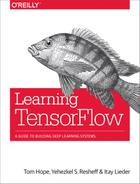
Consider, again, our example sentence: “Our company provides smart agriculture solutions for farms, with advanced AI, deep-learning.” We define (for simplicity) the context of a word as its immediate neighbors (“the company it keeps”)—i.e., the word to its left and the word to its right. So, the context of “company” is [our, provides], the context of “AI” is [advanced, deep-learning], and so on (see Figure 6-1).

Figure 6-1. Generating skip-grams from text.
In the skip-gram word2vec model, we train a model to predict context based on an input word. All that means in this case is that we generate training instance and label pairs such as (our, company), (provides, company), (advanced, AI), (deep-learning, AI), etc.
In addition to these pairs we extract from the data, we also sample “fake” pairs—that is, for a given input word (such as “AI”), we also sample random noise words as context (such as “monkeys”), in a process known as negative sampling. We use the true pairs combined with noise pairs to build our training instances and labels, which we use to train a binary classifier that learns to distinguish between them. The trainable parameters in this classifier are the vector representations—word embeddings. We tune these vectors to yield a classifier able to tell the difference between true contexts of a word and randomly sampled ones, in a binary classification setting.
TensorFlow enables many ways to implement the word2vec model, with increasing levels of sophistication and optimization, using multithreading and higher-level abstractions for optimized and shorter code. We present here a fundamental approach, which will introduce you to the core ideas and operations.
Let’s dive straight into implementing the core ideas in TensorFlow code.
Skip-Grams
We begin by preparing our data and extracting skip-grams. As in Chapter 5, our data comprises two classes of very short “sentences,” one composed of odd digits and the other of even digits (with numbers written in English). We make sentences equally sized here, for simplicity, but this doesn’t really matter for word2vec training. Let’s start by setting some parameters and creating sentences:
importosimportmathimportnumpyasnpimporttensorflowastffromtensorflow.contrib.tensorboard.pluginsimportprojectorbatch_size=64embedding_dimension=5negative_samples=8LOG_DIR="logs/word2vec_intro"digit_to_word_map={1:"One",2:"Two",3:"Three",4:"Four",5:"Five",6:"Six",7:"Seven",8:"Eight",9:"Nine"}sentences=[]# Create two kinds of sentences - sequences of odd and even digitsforiinrange(10000):rand_odd_ints=np.random.choice(range(1,10,2),3)sentences.append(" ".join([digit_to_word_map[r]forrinrand_odd_ints]))rand_even_ints=np.random.choice(range(2,10,2),3)sentences.append(" ".join([digit_to_word_map[r]forrinrand_even_ints]))
Let’s take a look at our sentences:
sentences[0:10]Out:['Seven One Five','Four Four Four','Five One Nine','Eight Two Eight','One Nine Three','Two Six Eight','Nine Seven Seven','Six Eight Six','One Five Five','Four Six Two']
Next, as in Chapter 5, we map words to indices by creating a dictionary with words as keys and indices as values, and create the inverse map:
# Map words to indicesword2index_map={}index=0forsentinsentences:forwordinsent.lower().split():ifwordnotinword2index_map:word2index_map[word]=indexindex+=1index2word_map={index:wordforword,indexinword2index_map.items()}vocabulary_size=len(index2word_map)
To prepare the data for word2vec, let’s create skip-grams:
# Generate skip-gram pairsskip_gram_pairs=[]forsentinsentences:tokenized_sent=sent.lower().split()foriinrange(1,len(tokenized_sent)-1):word_context_pair=[[word2index_map[tokenized_sent[i-1]],word2index_map[tokenized_sent[i+1]]],word2index_map[tokenized_sent[i]]]skip_gram_pairs.append([word_context_pair[1],word_context_pair[0][0]])skip_gram_pairs.append([word_context_pair[1],word_context_pair[0][1]])defget_skipgram_batch(batch_size):instance_indices=list(range(len(skip_gram_pairs)))np.random.shuffle(instance_indices)batch=instance_indices[:batch_size]x=[skip_gram_pairs[i][0]foriinbatch]y=[[skip_gram_pairs[i][1]]foriinbatch]returnx,y
Each skip-gram pair is composed of target and context word indices (given by the word2index_map dictionary, and not in correspondence to the actual digit each word represents). Let’s take a look:
skip_gram_pairs[0:10]Out:[[1,0],[1,2],[3,3],[3,3],[1,2],[1,4],[6,5],[6,5],[4,1],[4,7]]
We can generate batches of sequences of word indices, and check out the original sentences with the inverse dictionary we created earlier:
# Batch examplex_batch,y_batch=get_skipgram_batch(8)x_batchy_batch[index2word_map[word]forwordinx_batch][index2word_map[word[0]]forwordiny_batch]x_batchOut:[6,2,1,1,3,0,7,2]y_batchOut:[[5],[0],[4],[0],[5],[4],[1],[7]][index2word_map[word]forwordinx_batch]Out:['two','five','one','one','four','seven','three','five'][index2word_map[word[0]]forwordiny_batch]Out:['eight','seven','nine','seven','eight','nine','one','three']
Finally, we create our input and label placeholders:
# Input data, labelstrain_inputs=tf.placeholder(tf.int32,shape=[batch_size])train_labels=tf.placeholder(tf.int32,shape=[batch_size,1])
Embeddings in TensorFlow
In Chapter 5, we used the built-in tf.nn.embedding_lookup() function as part of our supervised RNN. The same functionality is used here. Here too, word embeddings can be viewed as lookup tables that map words to vector values, which are optimized as part of the training process to minimize a loss function. As we shall see in the next section, unlike in Chapter 5, here we use a loss function accounting for the unsupervised nature of the task, but the embedding lookup, which efficiently retrieves the vectors for each word in a given sequence of word indices, remains the same:
withtf.name_scope("embeddings"):embeddings=tf.Variable(tf.random_uniform([vocabulary_size,embedding_dimension],-1.0,1.0),name='embedding')# This is essentially a lookup tableembed=tf.nn.embedding_lookup(embeddings,train_inputs)
The Noise-Contrastive Estimation (NCE) Loss Function
In our introduction to skip-grams, we mentioned we create two types of context–target pairs of words: real ones that appear in the text, and “fake” noisy pairs that are generated by inserting random context words. Our goal is to learn to distinguish between the two, helping us learn a good word representation. We could draw random noisy context pairs ourselves, but luckily TensorFlow comes with a useful loss function designed especially for our task. tf.nn.nce_loss() automatically draws negative (“noise”) samples when we evaluate the loss (run it in a session):
# Create variables for the NCE lossnce_weights=tf.Variable(tf.truncated_normal([vocabulary_size,embedding_dimension],stddev=1.0/math.sqrt(embedding_dimension)))nce_biases=tf.Variable(tf.zeros([vocabulary_size]))loss=tf.reduce_mean(tf.nn.nce_loss(weights=nce_weights,biases=nce_biases,inputs=embed,labels=train_labels,num_sampled=negative_samples,num_classes=vocabulary_size))
We don’t go into the mathematical details of this loss function, but it is sufficient to think of it as a sort of efficient approximation to the ordinary softmax function used in classification tasks, as introduced in previous chapters. We tune our embedding vectors to optimize this loss function. For more details about it, see the official TensorFlow documentation and references within.
We’re now ready to train. In addition to obtaining our word embeddings in TensorFlow, we next introduce two useful capabilities: adjustment of the optimization learning rate, and interactive visualization of embeddings.
Learning Rate Decay
As discussed in previous chapters, gradient-descent optimization adjusts weights by making small steps in the direction that minimizes our loss function. The learning_rate hyperparameter controls just how aggressive these steps are. During gradient-descent training of a model, it is common practice to gradually make these steps smaller and smaller, so that we allow our optimization process to “settle down” as it approaches good points in the parameter space. This small addition to our training process can actually often lead to significant boosts in performance, and is a good practice to keep in mind in general.
tf.train.exponential_decay() applies exponential decay to the learning rate, with the exact form of decay controlled by a few hyperparameters, as seen in the following code (for exact details, see the official TensorFlow documentation at http://bit.ly/2tluxP1). Here, just as an example, we decay every 1,000 steps, and the decayed learning rate follows a staircase function—a piecewise constant function that resembles a staircase, as its name implies:
# Learning rate decayglobal_step=tf.Variable(0,trainable=False)learningRate=tf.train.exponential_decay(learning_rate=0.1,global_step=global_step,decay_steps=1000,decay_rate=0.95,staircase=True)train_step=tf.train.GradientDescentOptimizer(learningRate).minimize(loss)
Training and Visualizing with TensorBoard
We train our graph within a session as usual, adding some lines of code enabling cool interactive visualization in TensorBoard, a new tool for visualizing embeddings of high-dimensional data—typically images or word vectors—introduced for TensorFlow in late 2016.
First, we create a TSV (tab-separated values) metadata file. This file connects embedding vectors with associated labels or images we may have for them. In our case, each embedding vector has a label that is just the word it stands for.
We then point TensorBoard to our embedding variables (in this case, only one), and link them to the metadata file.
Finally, after completing optimization but before closing the session, we normalize the word embedding vectors to unit length, a standard post-processing step:
# Merge all summary opsmerged=tf.summary.merge_all()withtf.Session()assess:train_writer=tf.summary.FileWriter(LOG_DIR,graph=tf.get_default_graph())saver=tf.train.Saver()withopen(os.path.join(LOG_DIR,'metadata.tsv'),"w")asmetadata:metadata.write('NameClass')fork,vinindex2word_map.items():metadata.write('%s%d'%(v,k))config=projector.ProjectorConfig()embedding=config.embeddings.add()embedding.tensor_name=embeddings.name# Link embedding to its metadata fileembedding.metadata_path=os.path.join(LOG_DIR,'metadata.tsv')projector.visualize_embeddings(train_writer,config)tf.global_variables_initializer().run()forstepinrange(1000):x_batch,y_batch=get_skipgram_batch(batch_size)summary,_=sess.run([merged,train_step],feed_dict={train_inputs:x_batch,train_labels:y_batch})train_writer.add_summary(summary,step)ifstep%100==0:saver.save(sess,os.path.join(LOG_DIR,"w2v_model.ckpt"),step)loss_value=sess.run(loss,feed_dict={train_inputs:x_batch,train_labels:y_batch})("Loss at%d:%.5f"%(step,loss_value))# Normalize embeddings before usingnorm=tf.sqrt(tf.reduce_sum(tf.square(embeddings),1,keep_dims=True))normalized_embeddings=embeddings/normnormalized_embeddings_matrix=sess.run(normalized_embeddings)
Checking Out Our Embeddings
Let’s take a quick look at the word vectors we got. We select one word (one) and sort all the other word vectors by how close they are to it, in descending order:
ref_word=normalized_embeddings_matrix[word2index_map["one"]]cosine_dists=np.dot(normalized_embeddings_matrix,ref_word)ff=np.argsort(cosine_dists)[::-1][1:10]forfinff:(index2word_map[f])(cosine_dists[f])
Now let’s take a look at the word distances from the one vector:
Out:seven0.946973three0.938362nine0.755187five0.701269eight-0.0702622two-0.101749six-0.120306four-0.159601
We see that the word vectors representing odd numbers are similar (in terms of the dot product) to one, while those representing even numbers are not similar to it (and have a negative dot product with the one vector). We learned embedded vectors that allow us to distinguish between even and odd numbers—their respective vectors are far apart, and thus capture the context in which each word (odd or even digit) appeared.
Now, in TensorBoard, go to the Embeddings tab. This is a three-dimensional interactive visualization panel, where we can move around the space of our embedded vectors and explore different “angles,” zoom in, and more (see Figures 6-2 and 6-3). This enables us to understand our data and interpret the model in a visually comfortable manner. We can see, for instance, that the odd and even numbers occupy different areas in feature space.

Figure 6-2. Interactive visualization of word embeddings.

Figure 6-3. We can explore our word vectors from different angles (especially useful in high-dimensional problems with large vocabularies).
Of course, this type of visualization really shines when we have a great number of embedded vectors, such as in real text classification tasks with larger vocabularies, as we will see in Chapter 7, for example, or in the Embedding Projector TensorFlow demo. Here, we just give you a taste of how to interactively explore your data and deep learning models.
Pretrained Embeddings, Advanced RNN
As we discussed earlier, word embeddings are a powerful component in deep learning models for text. A popular approach seen in many applications is to first train word vectors with methods such as word2vec on massive amounts of (unlabeled) text, and then use these vectors in a downstream task such as supervised document classification.
In the previous section, we trained unsupervised word vectors from scratch. This approach typically requires very large corpora, such as Wikipedia entries or web pages. In practice, we often use pretrained word embeddings, trained on such huge corpora and available online, in much the same manner as the pretrained models presented in previous chapters.
In this section, we show how to use pretrained word embeddings in TensorFlow in a simplified text-classification task. To make things more interesting, we also take this opportunity to introduce some more useful and powerful components that are frequently used in modern deep learning applications for natural language understanding: the bidirectional RNN layers and the gated recurrent unit (GRU) cell.
We will expand and adapt our text-classification example from Chapter 5, focusing only on the parts that have changed.
Pretrained Word Embeddings
Here, we show how to take word vectors trained based on web data and incorporate them into a (contrived) text-classification task. The embedding method is known as GloVe, and while we don’t go into the details here, the overall idea is similar to that of word2vec—learning representations of words by the context in which they appear. Information on the method and its authors, and the pretrained vectors, is available on the project’s website.
We download the Common Crawl vectors (840B tokens), and proceed to our example.
We first set the path to the downloaded word vectors and some other parameters, as in Chapter 5:
importzipfileimportnumpyasnpimporttensorflowastfpath_to_glove="path/to/glove/file"PRE_TRAINED=TrueGLOVE_SIZE=300batch_size=128embedding_dimension=64num_classes=2hidden_layer_size=32times_steps=6
We then create the contrived, simple simulated data, also as in Chapter 5 (see details there):
digit_to_word_map={1:"One",2:"Two",3:"Three",4:"Four",5:"Five",6:"Six",7:"Seven",8:"Eight",9:"Nine"}digit_to_word_map[0]="PAD_TOKEN"even_sentences=[]odd_sentences=[]seqlens=[]foriinrange(10000):rand_seq_len=np.random.choice(range(3,7))seqlens.append(rand_seq_len)rand_odd_ints=np.random.choice(range(1,10,2),rand_seq_len)rand_even_ints=np.random.choice(range(2,10,2),rand_seq_len)ifrand_seq_len<6:rand_odd_ints=np.append(rand_odd_ints,[0]*(6-rand_seq_len))rand_even_ints=np.append(rand_even_ints,[0]*(6-rand_seq_len))even_sentences.append(" ".join([digit_to_word_map[r]forrinrand_odd_ints]))odd_sentences.append(" ".join([digit_to_word_map[r]forrinrand_even_ints]))data=even_sentences+odd_sentences# Same seq lengths for even, odd sentencesseqlens*=2labels=[1]*10000+[0]*10000foriinrange(len(labels)):label=labels[i]one_hot_encoding=[0]*2one_hot_encoding[label]=1labels[i]=one_hot_encoding
Next, we create the word index map:
word2index_map={}index=0forsentindata:forwordinsent.split():ifwordnotinword2index_map:word2index_map[word]=indexindex+=1index2word_map={index:wordforword,indexinword2index_map.items()}vocabulary_size=len(index2word_map)
Let’s refresh our memory of its content—just a map from word to an (arbitrary) index:
word2index_mapOut:{'Eight':7,'Five':1,'Four':6,'Nine':3,'One':5,'PAD_TOKEN':2,'Seven':4,'Six':9,'Three':0,'Two':8}
Now, we are ready to get word vectors. There are 2.2 million words in the vocabulary of the pretrained GloVe embeddings we downloaded, and in our toy example we have only 9. So, we take the GloVe vectors only for words that appear in our own tiny vocabulary:
defget_glove(path_to_glove,word2index_map):embedding_weights={}count_all_words=0withzipfile.ZipFile(path_to_glove)asz:withz.open("glove.840B.300d.txt")asf:forlineinf:vals=line.split()word=str(vals[0].decode("utf-8"))ifwordinword2index_map:(word)count_all_words+=1coefs=np.asarray(vals[1:],dtype='float32')coefs/=np.linalg.norm(coefs)embedding_weights[word]=coefsifcount_all_words==vocabulary_size-1:breakreturnembedding_weightsword2embedding_dict=get_glove(path_to_glove,word2index_map)
We go over the GloVe file line by line, take the word vectors we need, and normalize them. Once we have extracted the nine words we need, we stop the process and exit the loop. The output of our function is a dictionary, mapping from each word to its vector.
The next step is to place these vectors in a matrix, which is the required format for TensorFlow. In this matrix, each row index should correspond to the word index:
embedding_matrix=np.zeros((vocabulary_size,GLOVE_SIZE))forword,indexinword2index_map.items():ifnotword=="PAD_TOKEN":word_embedding=word2embedding_dict[word]embedding_matrix[index,:]=word_embedding
Note that for the PAD_TOKEN word, we set the corresponding vector to 0. As we saw in Chapter 5, we ignore padded tokens in our call to dynamic_rnn() by telling it the original sequence length.
We now create our training and test data:
data_indices=list(range(len(data)))np.random.shuffle(data_indices)data=np.array(data)[data_indices]labels=np.array(labels)[data_indices]seqlens=np.array(seqlens)[data_indices]train_x=data[:10000]train_y=labels[:10000]train_seqlens=seqlens[:10000]test_x=data[10000:]test_y=labels[10000:]test_seqlens=seqlens[10000:]defget_sentence_batch(batch_size,data_x,data_y,data_seqlens):instance_indices=list(range(len(data_x)))np.random.shuffle(instance_indices)batch=instance_indices[:batch_size]x=[[word2index_map[word]forwordindata_x[i].split()]foriinbatch]y=[data_y[i]foriinbatch]seqlens=[data_seqlens[i]foriinbatch]returnx,y,seqlens
And we create our input placeholders:
_inputs=tf.placeholder(tf.int32,shape=[batch_size,times_steps])embedding_placeholder=tf.placeholder(tf.float32,[vocabulary_size,GLOVE_SIZE])_labels=tf.placeholder(tf.float32,shape=[batch_size,num_classes])_seqlens=tf.placeholder(tf.int32,shape=[batch_size])
Note that we created an embedding_placeholder, to which we feed the word vectors:
ifPRE_TRAINED:embeddings=tf.Variable(tf.constant(0.0,shape=[vocabulary_size,GLOVE_SIZE]),trainable=True)# If using pretrained embeddings, assign them to the embeddings variableembedding_init=embeddings.assign(embedding_placeholder)embed=tf.nn.embedding_lookup(embeddings,_inputs)else:embeddings=tf.Variable(tf.random_uniform([vocabulary_size,embedding_dimension],-1.0,1.0))embed=tf.nn.embedding_lookup(embeddings,_inputs)
Our embeddings are initialized with the content of embedding_placeholder, using the assign() function to assign initial values to the embeddings variable. We set trainable=True to tell TensorFlow we want to update the values of the word vectors, by optimizing them for the task at hand. However, it is often useful to set trainable=False and not update these values; for example, when we do not have much labeled data or have reason to believe the word vectors are already “good” at capturing the patterns we are after.
There is one more step missing to fully incorporate the word vectors into the training—feeding embedding_placeholder with embedding_matrix. We will get to that soon, but for now we continue the graph building and introduce bidirectional RNN layers and GRU cells.
Bidirectional RNN and GRU Cells
Bidirectional RNN layers are a simple extension of the RNN layers we saw in Chapter 5. All they consist of, in their basic form, is two ordinary RNN layers: one layer that reads the sequence from left to right, and another that reads from right to left. Each yields a hidden representation, the left-to-right vector , and the right-to-left vector . These are then concatenated into one vector. The major advantage of this representation is its ability to capture the context of words from both directions, which enables richer understanding of natural language and the underlying semantics in text. In practice, in complex tasks, it often leads to improved accuracy. For example, in part-of-speech (POS) tagging, we want to output a predicted tag for each word in a sentence (such as “noun,” “adjective,” etc.). In order to predict a POS tag for a given word, it is useful to have information on its surrounding words, from both directions.
Gated recurrent unit (GRU) cells are a simplification of sorts of LSTM cells. They also have a memory mechanism, but with considerably fewer parameters than LSTM. They are often used when there is less available data, and are faster to compute. We do not go into the mathematical details here, as they are not important for our purposes; there are many good online resources explaining GRU and how it is different from LSTM.
TensorFlow comes equipped with tf.nn.bidirectional_dynamic_rnn(), which is an extension of dynamic_rnn() for bidirectional layers. It takes cell_fw and cell_bw RNN cells, which are the left-to-right and right-to-left vectors, respectively. Here we use GRUCell() for our forward and backward representations and add dropout for regularization, using the built-in DropoutWrapper():
withtf.name_scope("biGRU"):withtf.variable_scope('forward'):gru_fw_cell=tf.contrib.rnn.GRUCell(hidden_layer_size)gru_fw_cell=tf.contrib.rnn.DropoutWrapper(gru_fw_cell)withtf.variable_scope('backward'):gru_bw_cell=tf.contrib.rnn.GRUCell(hidden_layer_size)gru_bw_cell=tf.contrib.rnn.DropoutWrapper(gru_bw_cell)outputs,states=tf.nn.bidirectional_dynamic_rnn(cell_fw=gru_fw_cell,cell_bw=gru_bw_cell,inputs=embed,sequence_length=_seqlens,dtype=tf.float32,scope="BiGRU")states=tf.concat(values=states,axis=1)
We concatenate the forward and backward state vectors by using tf.concat() along the suitable axis, and then add a linear layer followed by softmax as in Chapter 5:
weights={'linear_layer':tf.Variable(tf.truncated_normal([2*hidden_layer_size,num_classes],mean=0,stddev=.01))}biases={'linear_layer':tf.Variable(tf.truncated_normal([num_classes],mean=0,stddev=.01))}# extract the final state and use in a linear layerfinal_output=tf.matmul(states,weights["linear_layer"])+biases["linear_layer"]softmax=tf.nn.softmax_cross_entropy_with_logits(logits=final_output,labels=_labels)cross_entropy=tf.reduce_mean(softmax)train_step=tf.train.RMSPropOptimizer(0.001,0.9).minimize(cross_entropy)correct_prediction=tf.equal(tf.argmax(_labels,1),tf.argmax(final_output,1))accuracy=(tf.reduce_mean(tf.cast(correct_prediction,tf.float32)))*100
We are now ready to train. We initialize the embedding_placeholder by feeding it our embedding_matrix. It’s important to note that we do so after calling tf.global_variables_initializer()—doing this in the reverse order would overrun the pre-trained vectors with a default initializer:
withtf.Session()assess:sess.run(tf.global_variables_initializer())sess.run(embedding_init,feed_dict={embedding_placeholder:embedding_matrix})forstepinrange(1000):x_batch,y_batch,seqlen_batch=get_sentence_batch(batch_size,train_x,train_y,train_seqlens)sess.run(train_step,feed_dict={_inputs:x_batch,_labels:y_batch,_seqlens:seqlen_batch})ifstep%100==0:acc=sess.run(accuracy,feed_dict={_inputs:x_batch,_labels:y_batch,_seqlens:seqlen_batch})("Accuracy at%d:%.5f"%(step,acc))fortest_batchinrange(5):x_test,y_test,seqlen_test=get_sentence_batch(batch_size,test_x,test_y,test_seqlens)batch_pred,batch_acc=sess.run([tf.argmax(final_output,1),accuracy],feed_dict={_inputs:x_test,_labels:y_test,_seqlens:seqlen_test})("Test batch accuracy%d:%.5f"%(test_batch,batch_acc))("Test batch accuracy%d:%.5f"%(test_batch,batch_acc))
Summary
In this chapter, we extended our knowledge regarding working with text sequences, adding some important tools to our TensorFlow toolbox. We saw a basic implementation of word2vec, learning the core concepts and ideas, and used TensorBoard for 3D interactive visualization of embeddings. We then incorporated publicly available GloVe word vectors, and RNN components that allow for richer and more efficient models. In the next chapter, we will see how to use abstraction libraries, including for classification tasks on real text data with LSTM networks.