Chapter 5. Text I: Working with Text and Sequences, and TensorBoard Visualization
In this chapter we show how to work with sequences in TensorFlow, and in particular text. We begin by introducing recurrent neural networks (RNNs), a powerful class of deep learning algorithms particularly useful and popular in natural language processing (NLP). We show how to implement RNN models from scratch, introduce some important TensorFlow capabilities, and visualize the model with the interactive TensorBoard. We then explore how to use an RNN in a supervised text classification problem with word-embedding training. Finally, we show how to build a more advanced RNN model with long short-term memory (LSTM) networks and how to handle sequences of variable length.
The Importance of Sequence Data
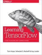
We saw in the previous chapter that using the spatial structure of images can lead to advanced models with excellent results. As discussed in that chapter, exploiting structure is the key to success. As we will see shortly, an immensely important and useful type of structure is the sequential structure. Thinking in terms of data science, this fundamental structure appears in many datasets, across all domains. In computer vision, video is a sequence of visual content evolving over time. In speech we have audio signals, in genomics gene sequences; we have longitudinal medical records in healthcare, financial data in the stock market, and so on (see Figure 5-1).

Figure 5-1. The ubiquity of sequence data.
A particularly important type of data with strong sequential structure is natural language—text data. Deep learning methods that exploit the sequential structure inherent in texts—characters, words, sentences, paragraphs, documents—are at the forefront of natural language understanding (NLU) systems, often leaving more traditional methods in the dust. There are a great many types of NLU tasks that are of interest to solve, ranging from document classification to building powerful language models, from answering questions automatically to generating human-level conversation agents. These tasks are fiendishly difficult, garnering the efforts and attention of the entire AI community in both academia and industry.
In this chapter, we focus on the basic building blocks and tasks, and show how to work with sequences—primarily of text—in TensorFlow. We take a detailed deep dive into the core elements of sequence models in TensorFlow, implementing some of them from scratch, to gain a thorough understanding. In the next chapter we show more advanced text modeling techniques with TensorFlow, and in Chapter 7 we use abstraction libraries that offer simpler, high-level ways to implement our models.
We begin with the most important and popular class of deep learning models for sequences (in particular, text): recurrent neural networks.
Introduction to Recurrent Neural Networks
Recurrent neural networks are a powerful and widely used class of neural network architectures for modeling sequence data. The basic idea behind RNN models is that each new element in the sequence contributes some new information, which updates the current state of the model.
In the previous chapter, which explored computer vision with CNN models, we discussed how those architectures are inspired by the current scientific perceptions of the way the human brain processes visual information. These scientific perceptions are often rather close to our commonplace intuition from our day-to-day lives about how we process sequential information.
When we receive new information, clearly our “history” and “memory” are not wiped out, but instead “updated.” When we read a sentence in some text, with each new word, our current state of information is updated, and it is dependent not only on the new observed word but on the words that preceded it.
A fundamental mathematical construct in statistics and probability, which is often used as a building block for modeling sequential patterns via machine learning is the Markov chain model. Figuratively speaking, we can view our data sequences as “chains,” with each node in the chain dependent in some way on the previous node, so that “history” is not erased but carried on.
RNN models are also based on this notion of chain structure, and vary in how exactly they maintain and update information. As their name implies, recurrent neural nets apply some form of “loop.” As seen in Figure 5-2, at some point in time t, the network observes an input xt (a word in a sentence) and updates its “state vector” to ht from the previous vector ht-1. When we process new input (the next word), it will be done in some manner that is dependent on ht and thus on the history of the sequence (the previous words we’ve seen affect our understanding of the current word). As seen in the illustration, this recurrent structure can simply be viewed as one long unrolled chain, with each node in the chain performing the same kind of processing “step” based on the “message” it obtains from the output of the previous node. This, of course, is very related to the Markov chain models discussed previously and their hidden Markov model (HMM) extensions, which are not discussed in this book.

Figure 5-2. Recurrent neural networks updating with new information received over time.
Vanilla RNN Implementation
In this section we implement a basic RNN from scratch, explore its inner workings, and gain insight into how TensorFlow can work with sequences. We introduce some powerful, fairly low-level tools that TensorFlow provides for working with sequence data, which you can use to implement your own systems.
In the next sections, we will show how to use higher-level TensorFlow RNN modules.
We begin with defining our basic model mathematically. This mainly consists of defining the recurrence structure—the RNN update step.
The update step for our simple vanilla RNN is
ht = tanh(Wxxt + Whht-1 + b)
where Wh, Wx, and b are weight and bias variables we learn, tanh(·) is the hyperbolic tangent function that has its range in [–1,1] and is strongly connected to the sigmoid function used in previous chapters, and xt and ht are the input and state vectors as defined previously. Finally, the hidden state vector is multiplied by another set of weights, yielding the outputs that appear in Figure 5-2.
MNIST images as sequences
To get a first taste of the power and general applicability of sequence models, in this section we implement our first RNN to solve the MNIST image classification task that you are by now familiar with. Later in this chapter we will focus on sequences of text, and see how neural sequence models can powerfully manipulate them and extract information to solve NLU tasks.
But, you may ask, what have images got to do with sequences?
As we saw in the previous chapter, the architecture of convolutional neural networks makes use of the spatial structure of images. While the structure of natural images is well suited for CNN models, it is revealing to look at the structure of images from different angles. In a trend in cutting-edge deep learning research, advanced models attempt to exploit various kinds of sequential structures in images, trying to capture in some sense the “generative process” that created each image. Intuitively, this all comes down to the notion that nearby areas in images are somehow related, and trying to model this structure.
Here, to introduce basic RNNs and how to work with sequences, we take a simple sequential view of images: we look at each image in our data as a sequence of rows (or columns). In our MNIST data, this just means that each 28×28-pixel image can be viewed as a sequence of length 28, each element in the sequence a vector of 28 pixels (see Figure 5-3). Then, the temporal dependencies in the RNN can be imaged as a scanner head, scanning the image from top to bottom (rows) or left to right (columns).

Figure 5-3. An image as a sequence of pixel columns.
We start by loading data, defining some parameters, and creating placeholders for our data:
importtensorflowastf# Import MNIST datafromtensorflow.examples.tutorials.mnistimportinput_datamnist=input_data.read_data_sets("/tmp/data/",one_hot=True)# Define some parameterselement_size=28time_steps=28num_classes=10batch_size=128hidden_layer_size=128# Where to save TensorBoard model summariesLOG_DIR="logs/RNN_with_summaries"# Create placeholders for inputs, labels_inputs=tf.placeholder(tf.float32,shape=[None,time_steps,element_size],name='inputs')y=tf.placeholder(tf.float32,shape=[None,num_classes],name='labels')
element_size is the dimension of each vector in our sequence—in our case, a row/column of 28 pixels. time_steps is the number of such elements in a sequence.
As we saw in previous chapters, when we load data with the built-in MNIST data loader, it comes in unrolled form—a vector of 784 pixels. When we load batches of data during training (we’ll get to that later in this section), we simply reshape each unrolled vector to [batch_size, time_steps, element_size]:
batch_x,batch_y=mnist.train.next_batch(batch_size)# Reshape data to get 28 sequences of 28 pixelsbatch_x=batch_x.reshape((batch_size,time_steps,element_size))
We set hidden_layer_size (arbitrarily to 128, controlling the size of the hidden RNN state vector discussed earlier.
LOG_DIR is the directory to which we save model summaries for TensorBoard visualization. You will learn what this means as we go.
TensorBoard visualizations
In this chapter, we will also briefly introduce TensorBoard visualizations. TensorBoard allows you to monitor and explore the model structure, weights, and training process, and requires some very simple additions to the code. More details are provided throughout this chapter and further along in the book.
Finally, our input and label placeholders are created with the suitable dimensions.
The RNN step
Let’s implement the mathematical model for the RNN step.
We first create a function used for logging summaries, which we will use later in TensorBoard to visualize our model and training process (it is not important to understand its technicalities at this stage):
# This helper function, taken from the official TensorFlow documentation,# simply adds some ops that take care of logging summariesdefvariable_summaries(var):withtf.name_scope('summaries'):mean=tf.reduce_mean(var)tf.summary.scalar('mean',mean)withtf.name_scope('stddev'):stddev=tf.sqrt(tf.reduce_mean(tf.square(var-mean)))tf.summary.scalar('stddev',stddev)tf.summary.scalar('max',tf.reduce_max(var))tf.summary.scalar('min',tf.reduce_min(var))tf.summary.histogram('histogram',var)
Next, we create the weight and bias variables used in the RNN step:
# Weights and bias for input and hidden layerwithtf.name_scope('rnn_weights'):withtf.name_scope("W_x"):Wx=tf.Variable(tf.zeros([element_size,hidden_layer_size]))variable_summaries(Wx)withtf.name_scope("W_h"):Wh=tf.Variable(tf.zeros([hidden_layer_size,hidden_layer_size]))variable_summaries(Wh)withtf.name_scope("Bias"):b_rnn=tf.Variable(tf.zeros([hidden_layer_size]))variable_summaries(b_rnn)
Applying the RNN step with tf.scan()
We now create a function that implements the vanilla RNN step we saw in the previous section using the variables we created. It should by now be straightforward to understand the TensorFlow code used here:
defrnn_step(previous_hidden_state,x):current_hidden_state=tf.tanh(tf.matmul(previous_hidden_state,Wh)+tf.matmul(x,Wx)+b_rnn)returncurrent_hidden_state
Next, we apply this function across all 28 time steps:
# Processing inputs to work with scan function# Current input shape: (batch_size, time_steps, element_size)processed_input=tf.transpose(_inputs,perm=[1,0,2])# Current input shape now: (time_steps, batch_size, element_size)initial_hidden=tf.zeros([batch_size,hidden_layer_size])# Getting all state vectors across timeall_hidden_states=tf.scan(rnn_step,processed_input,initializer=initial_hidden,name='states')
In this small code block, there are some important elements to understand. First, we reshape the inputs from [batch_size, time_steps, element_size] to [time_steps, batch_size, element_size]. The perm argument to tf.transpose() tells TensorFlow which axes we want to switch around. Now that the first axis in our input Tensor represents the time axis, we can iterate across all time steps by using the built-in tf.scan() function, which repeatedly applies a callable (function) to a sequence of elements in order, as explained in the following note.
tf.scan()
This important function was added to TensorFlow to allow us to introduce loops into the computation graph, instead of just “unrolling” the loops explicitly by adding more and more replications of the same operations. More technically, it is a higher-order function very similar to the reduce operator, but it returns all intermediate accumulator values over time. There are several advantages to this approach, chief among them the ability to have a dynamic number of iterations rather than fixed, computational speedups and optimizations for graph construction.
To demonstrate the use of this function, consider the following simple example (which is separate from the overall RNN code in this section):
importnumpyasnpimporttensorflowastfelems=np.array(["T","e","n","s","o","r"," ","F","l","o","w"])scan_sum=tf.scan(lambdaa,x:a+x,elems)sess=tf.InteractiveSession()sess.run(scan_sum)
Let’s see what we get:
array([b'T', b'Te', b'Ten', b'Tens', b'Tenso', b'Tensor', b'Tensor ',
       b'Tensor F', b'Tensor Fl', b'Tensor Flo', b'Tensor Flow'],
       dtype=object)
In this case, we use tf.scan() to sequentially concatenate characters to a string, in a manner analogous to the arithmetic cumulative sum.
Sequential outputs
As we saw earlier, in an RNN we get a state vector for each time step, multiply it by some weights, and get an output vector—our new representation of the data. Let’s implement this:
# Weights for output layerswithtf.name_scope('linear_layer_weights')asscope:withtf.name_scope("W_linear"):Wl=tf.Variable(tf.truncated_normal([hidden_layer_size,num_classes],mean=0,stddev=.01))variable_summaries(Wl)withtf.name_scope("Bias_linear"):bl=tf.Variable(tf.truncated_normal([num_classes],mean=0,stddev=.01))variable_summaries(bl)# Apply linear layer to state vectordefget_linear_layer(hidden_state):returntf.matmul(hidden_state,Wl)+blwithtf.name_scope('linear_layer_weights')asscope:# Iterate across time, apply linear layer to all RNN outputsall_outputs=tf.map_fn(get_linear_layer,all_hidden_states)# Get last outputoutput=all_outputs[-1]tf.summary.histogram('outputs',output)
Our input to the RNN is sequential, and so is our output. In this sequence classification example, we take the last state vector and pass it through a fully connected linear layer to extract an output vector (which will later be passed through a softmax activation function to generate predictions). This is common practice in basic sequence classification, where we assume that the last state vector has “accumulated” information representing the entire sequence.
To implement this, we first define the linear layer’s weights and bias term variables, and create a factory function for this layer. Then we apply this layer to all outputs with tf.map_fn(), which is pretty much the same as the typical map function that applies functions to sequences/iterables in an element-wise manner, in this case on each element in our sequence.
Finally, we extract the last output for each instance in the batch, with negative indexing (similarly to ordinary Python). We will see some more ways to do this later and investigate outputs and states in some more depth.
RNN classification
We’re now ready to train a classifier, much in the same way we did in the previous chapters. We define the ops for loss function computation, optimization, and prediction, add some more summaries for TensorBoard, and merge all these summaries into one operation:
withtf.name_scope('cross_entropy'):cross_entropy=tf.reduce_mean(tf.nn.softmax_cross_entropy_with_logits(logits=output,labels=y))tf.summary.scalar('cross_entropy',cross_entropy)withtf.name_scope('train'):# Using RMSPropOptimizertrain_step=tf.train.RMSPropOptimizer(0.001,0.9).minimize(cross_entropy)withtf.name_scope('accuracy'):correct_prediction=tf.equal(tf.argmax(y,1),tf.argmax(output,1))accuracy=(tf.reduce_mean(tf.cast(correct_prediction,tf.float32)))*100tf.summary.scalar('accuracy',accuracy)# Merge all the summariesmerged=tf.summary.merge_all()
By now you should be familiar with most of the components used for defining the loss function and optimization. Here, we used the RMSPropOptimizer, implementing a well-known and strong gradient descent algorithm, with some standard hyperparameters. Of course, we could have used any other optimizer (and do so throughout this book!).
We create a small test set with unseen MNIST images, and add some more technical ops and commands for logging summaries that we will use in TensorBoard.
Let’s run the model and check out the results:
# Get a small test settest_data=mnist.test.images[:batch_size].reshape((-1,time_steps,element_size))test_label=mnist.test.labels[:batch_size]withtf.Session()assess:# Write summaries to LOG_DIR -- used by TensorBoardtrain_writer=tf.summary.FileWriter(LOG_DIR+'/train',graph=tf.get_default_graph())test_writer=tf.summary.FileWriter(LOG_DIR+'/test',graph=tf.get_default_graph())sess.run(tf.global_variables_initializer())foriinrange(10000):batch_x,batch_y=mnist.train.next_batch(batch_size)# Reshape data to get 28 sequences of 28 pixelsbatch_x=batch_x.reshape((batch_size,time_steps,element_size))summary,_=sess.run([merged,train_step],feed_dict={_inputs:batch_x,y:batch_y})# Add to summariestrain_writer.add_summary(summary,i)ifi%1000==0:acc,loss,=sess.run([accuracy,cross_entropy],feed_dict={_inputs:batch_x,y:batch_y})("Iter "+str(i)+", Minibatch Loss= "+"{:.6f}".format(loss)+", Training Accuracy= "+"{:.5f}".format(acc))ifi%10:# Calculate accuracy for 128 MNIST test images and# add to summariessummary,acc=sess.run([merged,accuracy],feed_dict={_inputs:test_data,y:test_label})test_writer.add_summary(summary,i)test_acc=sess.run(accuracy,feed_dict={_inputs:test_data,y:test_label})("Test Accuracy:",test_acc)
Finally, we print some training and testing accuracy results:
Iter0,MinibatchLoss=2.303386,TrainingAccuracy=7.03125Iter1000,MinibatchLoss=1.238117,TrainingAccuracy=52.34375Iter2000,MinibatchLoss=0.614925,TrainingAccuracy=85.15625Iter3000,MinibatchLoss=0.439684,TrainingAccuracy=82.81250Iter4000,MinibatchLoss=0.077756,TrainingAccuracy=98.43750Iter5000,MinibatchLoss=0.220726,TrainingAccuracy=89.84375Iter6000,MinibatchLoss=0.015013,TrainingAccuracy=100.00000Iter7000,MinibatchLoss=0.017689,TrainingAccuracy=100.00000Iter8000,MinibatchLoss=0.065443,TrainingAccuracy=99.21875Iter9000,MinibatchLoss=0.071438,TrainingAccuracy=98.43750TestingAccuracy:97.6563
To summarize this section, we started off with the raw MNIST pixels and regarded them as sequential data—each column (or row) of 28 pixels as a time step. We then applied the vanilla RNN to extract outputs corresponding to each time-step and used the last output to perform classification of the entire sequence (image).
Visualizing the model with TensorBoard
TensorBoard is an interactive browser-based tool that allows us to visualize the learning process, as well as explore our trained model.
To run TensorBoard, go to the command terminal and tell TensorBoard where the relevant summaries you logged are:
tensorboard--logdir=LOG_DIR
Here, LOG_DIR should be replaced with your log directory. If you are on Windows and this is not working, make sure you are running the terminal from the same drive where the log data is, and add a name to the log directory as follows in order to bypass a bug in the way TensorBoard parses the path:
tensorboard--logdir=rnn_demo:LOG_DIR
TensorBoard allows us to assign names to individual log directories by putting a colon between the name and the path, which may be useful when working with multiple log directories. In such a case, we pass a comma-separated list of log directories as follows:
tensorboard--logdir=rnn_demo1:LOG_DIR1,rnn_demo2:LOG_DIR2
In our example (with one log directory), once you have run the tensorboard command, you should get something like the following, telling you where to navigate in your browser:
StartingTensorBoardb'39'onport6006(Youcannavigatetohttp://10.100.102.4:6006)
If the address does not work, go to localhost:6006, which should always work.
TensorBoard recursively walks the directory tree rooted at LOG_DIR looking for subdirectories that contain tfevents log data. If you run this example multiple times, make sure to either delete the LOG_DIR folder you created after each run, or write the logs to separate subdirectories within LOG_DIR, such as LOG_DIR/run1/train, LOG_DIR/run2/train, and so forth, to avoid issues with overwriting log files, which may lead to some “funky” plots.
Let’s take a look at some of the visualizations we can get. In the next section, we will explore interactive visualization of high-dimensional data with TensorBoard—for now, we focus on plotting training process summaries and trained weights.
First, in your browser, go to the Scalars tab. Here TensorBoard shows us summaries of all scalars, including not only training and testing accuracy, which are usually most interesting, but also some summary statistics we logged about variables (see Figure 5-4). Hovering over the plots, we can see some numerical figures.

Figure 5-4. TensorBoard scalar summaries.
In the Graphs tab we can get an interactive visualization of our computation graph, from a high-level view down to the basic ops, by zooming in (see Figure 5-5).

Figure 5-5. Zooming in on the computation graph.
Finally, in the Histograms tab we see histograms of our weights across the training process (see Figure 5-6). Of course, we had to explicitly add these histograms to our logging in order to view them, with tf.summary.histogram().

Figure 5-6. Histograms of weights throughout the learning process.
TensorFlow Built-in RNN Functions
The preceding example taught us some of the fundamental and powerful ways we can work with sequences, by implementing our graph pretty much from scratch. In practice, it is of course a good idea to use built-in higher-level modules and functions. This not only makes the code shorter and easier to write, but exploits many low-level optimizations afforded by TensorFlow implementations.
In this section we first present a new, shorter version of the code in its entirety. Since most of the overall details have not changed, we focus on the main new elements, tf.contrib.rnn.BasicRNNCell and tf.nn.dynamic_rnn():
importtensorflowastffromtensorflow.examples.tutorials.mnistimportinput_datamnist=input_data.read_data_sets("/tmp/data/",one_hot=True)element_size=28;time_steps=28;num_classes=10batch_size=128;hidden_layer_size=128_inputs=tf.placeholder(tf.float32,shape=[None,time_steps,element_size],name='inputs')y=tf.placeholder(tf.float32,shape=[None,num_classes],name='inputs')# TensorFlow built-in functionsrnn_cell=tf.contrib.rnn.BasicRNNCell(hidden_layer_size)outputs,_=tf.nn.dynamic_rnn(rnn_cell,_inputs,dtype=tf.float32)Wl=tf.Variable(tf.truncated_normal([hidden_layer_size,num_classes],mean=0,stddev=.01))bl=tf.Variable(tf.truncated_normal([num_classes],mean=0,stddev=.01))defget_linear_layer(vector):returntf.matmul(vector,Wl)+bllast_rnn_output=outputs[:,-1,:]final_output=get_linear_layer(last_rnn_output)softmax=tf.nn.softmax_cross_entropy_with_logits(logits=final_output,labels=y)cross_entropy=tf.reduce_mean(softmax)train_step=tf.train.RMSPropOptimizer(0.001,0.9).minimize(cross_entropy)correct_prediction=tf.equal(tf.argmax(y,1),tf.argmax(final_output,1))accuracy=(tf.reduce_mean(tf.cast(correct_prediction,tf.float32)))*100sess=tf.InteractiveSession()sess.run(tf.global_variables_initializer())test_data=mnist.test.images[:batch_size].reshape((-1,time_steps,element_size))test_label=mnist.test.labels[:batch_size]foriinrange(3001):batch_x,batch_y=mnist.train.next_batch(batch_size)batch_x=batch_x.reshape((batch_size,time_steps,element_size))sess.run(train_step,feed_dict={_inputs:batch_x,y:batch_y})ifi%1000==0:acc=sess.run(accuracy,feed_dict={_inputs:batch_x,y:batch_y})loss=sess.run(cross_entropy,feed_dict={_inputs:batch_x,y:batch_y})("Iter "+str(i)+", Minibatch Loss= "+"{:.6f}".format(loss)+", Training Accuracy= "+"{:.5f}".format(acc))("Testing Accuracy:",sess.run(accuracy,feed_dict={_inputs:test_data,y:test_label}))
tf.contrib.rnn.BasicRNNCell and tf.nn.dynamic_rnn()
TensorFlow’s RNN cells are abstractions that represent the basic operations each recurrent “cell” carries out (see Figure 5-2 at the start of this chapter for an illustration), and its associated state. They are, in general terms, a “replacement” of the rnn_step() function and the associated variables it required. Of course, there are many variants and types of cells, each with many methods and properties. We will see some more advanced cells toward the end of this chapter and later in the book.
Once we have created the rnn_cell, we feed it into tf.nn.dynamic_rnn(). This function replaces tf.scan() in our vanilla implementation and creates an RNN specified by rnn_cell.
As of this writing, in early 2017, TensorFlow includes a static and a dynamic function for creating an RNN. What does this mean? The static version creates an unrolled graph (as in Figure 5-2) of fixed length. The dynamic version uses a tf.While loop to dynamically construct the graph at execution time, leading to faster graph creation, which can be significant. This dynamic construction can also be very useful in other ways, some of which we will touch on when we discuss variable-length sequences toward the end of this chapter.
Note that contrib refers to the fact that code in this library is contributed and still requires testing. We discuss the contrib library in much more detail in Chapter 7. BasicRNNCell was moved to contrib in TensorFlow 1.0 as part of ongoing development. In version 1.2, many of the RNN functions and classes were moved back to the core namespace with aliases kept in contrib for backward compatibiliy, meaning that the preceding code works for all versions 1.X as of this writing.
RNN for Text Sequences
We began this chapter by learning how to implement RNN models in TensorFlow. For ease of exposition, we showed how to implement and use an RNN for a sequence made of pixels in MNIST images. We next show how to use these sequence models on text sequences.
Text data has some properties distinctly different from image data, which we will discuss here and later in this book. These properties can make it somewhat difficult to handle text data at first, and text data always requires at least some basic pre-processing steps for us to be able to work with it. To introduce working with text in TensorFlow, we will thus focus on the core components and create a minimal, contrived text dataset that will let us get straight to the action. In Chapter 7, we will apply RNN models to movie review sentiment classification.
Let’s get started, presenting our example data and discussing some key properties of text datasets as we go.
Text Sequences
In the MNIST RNN example we saw earlier, each sequence was of fixed size—the width (or height) of an image. Each element in the sequence was a dense vector of 28 pixels. In NLP tasks and datasets, we have a different kind of “picture.”
Our sequences could be of words forming a sentence, of sentences forming a paragraph, or even of characters forming words or paragraphs forming whole documents.
Consider the following sentence: “Our company provides smart agriculture solutions for farms, with advanced AI, deep-learning.” Say we obtain this sentence from an online news blog, and wish to process it as part of our machine learning system.
Each of the words in this sentence would be represented with an ID—an integer, commonly referred to as a token ID in NLP. So, the word “agriculture” could, for instance, be mapped to the integer 3452, the word “farm” to 12, “AI” to 150, and “deep-learning” to 0. This representation in terms of integer identifiers is very different from the vector of pixels in image data, in multiple ways. We will elaborate on this important point shortly when we discuss word embeddings, and in Chapter 6.
To make things more concrete, let’s start by creating our simplified text data.
Our simulated data consists of two classes of very short “sentences,” one composed of odd digits and the other of even digits (with numbers written in English). We generate sentences built of words representing even and odd numbers. Our goal is to learn to classify each sentence as either odd or even in a supervised text-classification task.
Of course, we do not really need any machine learning for this simple task—we use this contrived example only for illustrative purposes.
First, we define some constants, which will be explained as we go:
importnumpyasnpimporttensorflowastfbatch_size=128;embedding_dimension=64;num_classes=2hidden_layer_size=32;times_steps=6;element_size=1
Next, we create sentences. We sample random digits and map them to the corresponding “words” (e.g., 1 is mapped to “One,” 7 to “Seven,” etc.).
Text sequences typically have variable lengths, which is of course the case for all real natural language data (such as in the sentences appearing on this page).
To make our simulated sentences have different lengths, we sample for each sentence a random length between 3 and 6 with np.random.choice(range(3, 7))—the lower bound is inclusive, and the upper bound is exclusive.
Now, to put all our input sentences in one tensor (per batch of data instances), we need them to somehow be of the same size—so we pad sentences with a length shorter than 6 with zeros (or PAD symbols) to make all sentences equally sized (artificially). This pre-processing step is known as zero-padding. The following code accomplishes all of this:
digit_to_word_map={1:"One",2:"Two",3:"Three",4:"Four",5:"Five",6:"Six",7:"Seven",8:"Eight",9:"Nine"}digit_to_word_map[0]="PAD"even_sentences=[]odd_sentences=[]seqlens=[]foriinrange(10000):rand_seq_len=np.random.choice(range(3,7))seqlens.append(rand_seq_len)rand_odd_ints=np.random.choice(range(1,10,2),rand_seq_len)rand_even_ints=np.random.choice(range(2,10,2),rand_seq_len)# Paddingifrand_seq_len<6:rand_odd_ints=np.append(rand_odd_ints,[0]*(6-rand_seq_len))rand_even_ints=np.append(rand_even_ints,[0]*(6-rand_seq_len))even_sentences.append(" ".join([digit_to_word_map[r]forrinrand_odd_ints]))odd_sentences.append(" ".join([digit_to_word_map[r]forrinrand_even_ints]))data=even_sentences+odd_sentences# Same seq lengths for even, odd sentencesseqlens*=2
Let’s take a look at our sentences, each padded to length 6:
even_sentences[0:6]Out:['Four Four Two Four Two PAD','Eight Six Four PAD PAD PAD','Eight Two Six Two PAD PAD','Eight Four Four Eight PAD PAD','Eight Eight Four PAD PAD PAD','Two Two Eight Six Eight Four']
odd_sentences[0:6]Out:['One Seven Nine Three One PAD','Three Nine One PAD PAD PAD','Seven Five Three Three PAD PAD','Five Five Three One PAD PAD','Three Three Five PAD PAD PAD','Nine Three Nine Five Five Three']
Notice that we add the PAD word (token) to our data and digit_to_word_map dictionary, and separately store even and odd sentences and their original lengths (before padding).
Let’s take a look at the original sequence lengths for the sentences we printed:
seqlens[0:6]Out:[5,3,4,4,3,6]
Why keep the original sentence lengths? By zero-padding, we solved one technical problem but created another: if we naively pass these padded sentences through our RNN model as they are, it will process useless PAD symbols. This would both harm model correctness by processing “noise” and increase computation time. We resolve this issue by first storing the original lengths in the seqlens array and then telling TensorFlow’s tf.nn.dynamic_rnn() where each sentence ends.
In this chapter, our data is simulated—generated by us. In real applications, we would start off by getting a collection of documents (e.g., one-sentence tweets) and then mapping each word to an integer ID.
So, we now map words to indices—word identifiers—by simply creating a dictionary with words as keys and indices as values. We also create the inverse map. Note that there is no correspondence between the word IDs and the digits each word represents—the IDs carry no semantic meaning, just as in any NLP application with real data:
# Map from words to indicesword2index_map={}index=0forsentindata:forwordinsent.lower().split():ifwordnotinword2index_map:word2index_map[word]=indexindex+=1# Inverse mapindex2word_map={index:wordforword,indexinword2index_map.items()}vocabulary_size=len(index2word_map)
This is a supervised classification task—we need an array of labels in the one-hot format, train and test sets, a function to generate batches of instances, and placeholders, as usual.
First, we create the labels and split the data into train and test sets:
labels=[1]*10000+[0]*10000foriinrange(len(labels)):label=labels[i]one_hot_encoding=[0]*2one_hot_encoding[label]=1labels[i]=one_hot_encodingdata_indices=list(range(len(data)))np.random.shuffle(data_indices)data=np.array(data)[data_indices]labels=np.array(labels)[data_indices]seqlens=np.array(seqlens)[data_indices]train_x=data[:10000]train_y=labels[:10000]train_seqlens=seqlens[:10000]test_x=data[10000:]test_y=labels[10000:]test_seqlens=seqlens[10000:]
Next, we create a function that generates batches of sentences. Each sentence in a batch is simply a list of integer IDs corresponding to words:
defget_sentence_batch(batch_size,data_x,data_y,data_seqlens):instance_indices=list(range(len(data_x)))np.random.shuffle(instance_indices)batch=instance_indices[:batch_size]x=[[word2index_map[word]forwordindata_x[i].lower().split()]foriinbatch]y=[data_y[i]foriinbatch]seqlens=[data_seqlens[i]foriinbatch]returnx,y,seqlens
Finally, we create placeholders for data:
_inputs=tf.placeholder(tf.int32,shape=[batch_size,times_steps])_labels=tf.placeholder(tf.float32,shape=[batch_size,num_classes])# seqlens for dynamic calculation_seqlens=tf.placeholder(tf.int32,shape=[batch_size])
Note that we have created a placeholder for the original sequence lengths. We will see how to make use of these in our RNN shortly.
Supervised Word Embeddings
Our text data is now encoded as lists of word IDs—each sentence is a sequence of integers corresponding to words. This type of atomic representation, where each word is represented with an ID, is not scalable for training deep learning models with large vocabularies that occur in real problems. We could end up with millions of such word IDs, each encoded in one-hot (binary) categorical form, leading to great data sparsity and computational issues. We will discuss this in more depth in Chapter 6.
A powerful approach to work around this issue is to use word embeddings. The embedding is, in a nutshell, simply a mapping from high-dimensional one-hot vectors encoding words to lower-dimensional dense vectors. So, for example, if our vocabulary has size 100,000, each word in one-hot representation would be of the same size. The corresponding word vector—or word embedding—would be of size 300, say. The high-dimensional one-hot vectors are thus “embedded” into a continuous vector space with a much lower dimensionality.
In Chapter 6 we dive deeper into word embeddings, exploring a popular method to train them in an “unsupervised” manner known as word2vec.
Here, our end goal is to solve a text classification problem, and we will train word vectors in a supervised framework, tuning the embedded word vectors to solve the downstream classification task.
It is helpful to think of word embeddings as basic hash tables or lookup tables, mapping words to their dense vector values. These vectors are optimized as part of the training process. Previously, we gave each word an integer index, and sentences are then represented as sequences of these indices. Now, to obtain a word’s vector, we use the built-in tf.nn.embedding_lookup() function, which efficiently retrieves the vectors for each word in a given sequence of word indices:
withtf.name_scope("embeddings"):embeddings=tf.Variable(tf.random_uniform([vocabulary_size,embedding_dimension],-1.0,1.0),name='embedding')embed=tf.nn.embedding_lookup(embeddings,_inputs)
We will see examples of and visualizations of our vector representations of words shortly.
LSTM and Using Sequence Length
In the introductory RNN example with which we began, we implemented and used the basic vanilla RNN model. In practice, we often use slightly more advanced RNN models, which differ mainly by how they update their hidden state and propagate information through time. A very popular recurrent network is the long short-term memory (LSTM) network. It differs from vanilla RNN by having some special memory mechanisms that enable the recurrent cells to better store information for long periods of time, thus allowing them to capture long-term dependencies better than plain RNN.
There is nothing mysterious about these memory mechanisms; they simply consist of some more parameters added to each recurrent cell, enabling the RNN to overcome optimization issues and propagate information. These trainable parameters act as filters that select what information is worth “remembering” and passing on, and what is worth “forgetting.” They are trained in exactly the same way as any other parameter in a network, with gradient-descent algorithms and backpropagation. We don’t go into the more technical mathematical formulations here, but there are plenty of great resources out there delving into the details.
We create an LSTM cell with tf.contrib.rnn.BasicLSTMCell() and feed it to tf.nn.dynamic_rnn(), just as we did at the start of this chapter. We also give dynamic_rnn() the length of each sequence in a batch of examples, using the _seqlens placeholder we created earlier. TensorFlow uses this to stop all RNN steps beyond the last real sequence element. It also returns all output vectors over time (in the outputs tensor), which are all zero-padded beyond the true end of the sequence. So, for example, if the length of our original sequence is 5 and we zero-pad it to a sequence of length 15, the output for all time steps beyond 5 will be zero:
withtf.variable_scope("lstm"):lstm_cell=tf.contrib.rnn.BasicLSTMCell(hidden_layer_size,forget_bias=1.0)outputs,states=tf.nn.dynamic_rnn(lstm_cell,embed,sequence_length=_seqlens,dtype=tf.float32)weights={'linear_layer':tf.Variable(tf.truncated_normal([hidden_layer_size,num_classes],mean=0,stddev=.01))}biases={'linear_layer':tf.Variable(tf.truncated_normal([num_classes],mean=0,stddev=.01))}# Extract the last relevant output and use in a linear layerfinal_output=tf.matmul(states[1],weights["linear_layer"])+biases["linear_layer"]softmax=tf.nn.softmax_cross_entropy_with_logits(logits=final_output,labels=_labels)cross_entropy=tf.reduce_mean(softmax)
We take the last valid output vector—in this case conveniently available for us in the states tensor returned by dynamic_rnn()—and pass it through a linear layer (and the softmax function), using it as our final prediction. We will explore the concepts of last relevant output and zero-padding further in the next section, when we look at some outputs generated by dynamic_rnn() for our example sentences.
Training Embeddings and the LSTM Classifier
We have all the pieces in the puzzle. Let’s put them together, and complete an end-to-end training of both word vectors and a classification model:
train_step=tf.train.RMSPropOptimizer(0.001,0.9).minimize(cross_entropy)correct_prediction=tf.equal(tf.argmax(_labels,1),tf.argmax(final_output,1))accuracy=(tf.reduce_mean(tf.cast(correct_prediction,tf.float32)))*100withtf.Session()assess:sess.run(tf.global_variables_initializer())forstepinrange(1000):x_batch,y_batch,seqlen_batch=get_sentence_batch(batch_size,train_x,train_y,train_seqlens)sess.run(train_step,feed_dict={_inputs:x_batch,_labels:y_batch,_seqlens:seqlen_batch})ifstep%100==0:acc=sess.run(accuracy,feed_dict={_inputs:x_batch,_labels:y_batch,_seqlens:seqlen_batch})("Accuracy at%d:%.5f"%(step,acc))fortest_batchinrange(5):x_test,y_test,seqlen_test=get_sentence_batch(batch_size,test_x,test_y,test_seqlens)batch_pred,batch_acc=sess.run([tf.argmax(final_output,1),accuracy],feed_dict={_inputs:x_test,_labels:y_test,_seqlens:seqlen_test})("Test batch accuracy%d:%.5f"%(test_batch,batch_acc))output_example=sess.run([outputs],feed_dict={_inputs:x_test,_labels:y_test,_seqlens:seqlen_test})states_example=sess.run([states[1]],feed_dict={_inputs:x_test,_labels:y_test,_seqlens:seqlen_test})
As we can see, this is a pretty simple toy text classification problem:
Accuracy at 0: 32.81250
Accuracy at 100: 100.00000
Accuracy at 200: 100.00000
Accuracy at 300: 100.00000
Accuracy at 400: 100.00000
Accuracy at 500: 100.00000
Accuracy at 600: 100.00000
Accuracy at 700: 100.00000
Accuracy at 800: 100.00000
Accuracy at 900: 100.00000
Test batch accuracy 0: 100.00000
Test batch accuracy 1: 100.00000
Test batch accuracy 2: 100.00000
Test batch accuracy 3: 100.00000
Test batch accuracy 4: 100.00000
We’ve also computed an example batch of outputs generated by dynamic_rnn(), to further illustrate the concepts of zero-padding and last relevant outputs discussed in the previous section.
Let’s take a look at one example of these outputs, for a sentence that was zero-padded (in your random batch of data you may see different output, of course—look for a sentence whose seqlen was lower than the maximal 6):
seqlen_test[1]Out:4
output_example[0][1].shapeOut:(6,32)
This output has, as expected, six time steps, each a vector of size 32. Let’s take a glimpse at its values (printing only the first few dimensions to avoid clutter):
output_example[0][1][:6,0:3]Out:array([[-0.44493711,-0.51363373,-0.49310589],[-0.72036862,-0.68590945,-0.73340571],[-0.83176643,-0.78206956,-0.87831545],[-0.87982416,-0.82784462,-0.91132098],[0.,0.,0.],[0.,0.,0.]],dtype=float32)
We see that for this sentence, whose original length was 4, the last two time steps have zero vectors due to padding.
Finally, we look at the states vector returned by dynamic_rnn():
states_example[0][1][0:3]Out:array([-0.87982416,-0.82784462,-0.91132098],dtype=float32)
We can see that it conveniently stores for us the last relevant output vector—its values match the last relevant output vector before zero-padding.
At this point, you may be wondering how to access and manipulate the word vectors and explore the trained representation. We show how to do so, including interactive embedding visualization, in the next chapter.
Stacking multiple LSTMs
Earlier, we focused on a one-layer LSTM network for ease of exposition. Adding more layers is straightforward, using the MultiRNNCell() wrapper that combines multiple RNN cells into one multilayer cell.
Say, for example, we wanted to stack two LSTM layers in the preceding example. We can do this as follows:
num_LSTM_layers=2withtf.variable_scope("lstm"):lstm_cell_list=[tf.contrib.rnn.BasicLSTMCell(hidden_layer_size,forget_bias=1.0)foriiinrange(num_LSTM_layers)]cell=tf.contrib.rnn.MultiRNNCell(cells=lstm_cell_list,state_is_tuple=True)outputs,states=tf.nn.dynamic_rnn(cell,embed,sequence_length=_seqlens,dtype=tf.float32)
We first define an LSTM cell as before, and then feed it into the tf.contrib.rnn.MultiRNNCell() wrapper.
Now our network has two layers of LSTM, causing some shape issues when trying to extract the final state vectors. To get the final state of the second layer, we simply adapt our indexing a bit:
# Extract the final state and use in a linear layerfinal_output=tf.matmul(states[num_LSTM_layers-1][1],weights["linear_layer"])+biases["linear_layer"]
Summary
In this chapter we introduced sequence models in TensorFlow. We saw how to implement a basic RNN model from scratch by using tf.scan() and built-in modules, as well as more advanced LSTM networks, for both text and image data. Finally, we trained an end-to-end text classification RNN with word embeddings, and showed how to handle sequences of variable length. In the next chapter, we dive deeper into word embeddings and word2vec. In Chapter 7, we will see some cool abstraction layers over TensorFlow, and how they can be used to train advanced text classification RNN models with considerably less effort.