Chapter 10. Exporting and Serving Models with TensorFlow
In this chapter we will learn how to save and export models by using both simple and advanced production-ready methods. For the latter we introduce TensorFlow Serving, one of TensorFlow’s most practical tools for creating production environments. We start this chapter with a quick overview of two simple ways to save models and variables: first by manually saving the weights and reassigning them, and then by using the Saver class that creates training checkpoints for our variables and also exports our model. Finally, we shift to more advanced applications where we can deploy our model on a server by using TensorFlow Serving.
Saving and Exporting Our Model
So far we’ve dealt with how to create, train, and track models with TensorFlow. Now we will see how to save a trained model. Saving the current state of our weights is crucial for obvious practical reasons—we don’t want to have to retrain our model from scratch every time, and we also want a convenient way to share the state of our model with others (as in the pretrained models we saw in Chapter 7).
In this section we go over the basics of saving and exporting. We start with a simple way of saving and loading our weights to and from files. Then we will see how to use TensorFlow’s Saver object to keep serialized model checkpoints that include information about both the state of our weights and our constructed graph.
Assigning Loaded Weights
A naive but practical way to reuse our weights after training is saving them to a file, which we can later load to have them reassigned to the model.
Let’s look at some examples. Say we wish to save the weights of the basic softmax model used for the MNIST data in Chapter 2. After fetching them from the session, we have the weights represented as a NumPy array, and we save them in some format of our choice:
importnumpyasnpweights=sess.run(W)np.savez(os.path.join(path,'weight_storage'),weights)
Given that we have the exact same graph constructed, we can then load the file and assign the loaded weight values to the corresponding variables by using the .assign() method within a session:
loaded_w=np.load(path+'weight_storage.npz')loaded_w=loaded_w.items()[0][1]x=tf.placeholder(tf.float32,[None,784])W=tf.Variable(tf.zeros([784,10]))y_true=tf.placeholder(tf.float32,[None,10])y_pred=tf.matmul(x,W)cross_entropy=tf.reduce_mean(tf.nn.softmax_cross_entropy_with_logits(logits=y_pred,labels=y_true))gd_step=tf.train.GradientDescentOptimizer(0.5).minimize(cross_entropy)correct_mask=tf.equal(tf.argmax(y_pred,1),tf.argmax(y_true,1))accuracy=tf.reduce_mean(tf.cast(correct_mask,tf.float32))withtf.Session()assess:# Assigning loaded weightssess.run(W.assign(loaded_w))acc=sess.run(accuracy,feed_dict={x:data.test.images,y_true:data.test.labels})("Accuracy: {}".format(acc))Out:Accuracy:0.9199
Next, we will perform the same procedure, but this time for the CNN model used for the MNIST data in Chapter 4. Here we have eight different sets of weights: two filter weights and their corresponding biases for the convolution layers 1 and 2, and two sets of weights and biases for the fully connected layer. We encapsulate the model inside a class so we can conveniently keep an updated list of these eight parameters.
We also add optional arguments for weights to load:
ifweightsisnotNoneandsessisnotNone:self.load_weights(weights,sess)
and a function to assign their values when weights are passed:
defload_weights(self,weights,sess):fori,winenumerate(weights):("Weight index: {}".format(i),"Weight shape: {}".format(w.shape))sess.run(self.parameters[i].assign(w))
In its entirety:
classsimple_cnn:def__init__(self,x_image,keep_prob,weights=None,sess=None):self.parameters=[]self.x_image=x_imageconv1=self.conv_layer(x_image,shape=[5,5,1,32])conv1_pool=self.max_pool_2x2(conv1)conv2=self.conv_layer(conv1_pool,shape=[5,5,32,64])conv2_pool=self.max_pool_2x2(conv2)conv2_flat=tf.reshape(conv2_pool,[-1,7*7*64])full_1=tf.nn.relu(self.full_layer(conv2_flat,1024))full1_drop=tf.nn.dropout(full_1,keep_prob=keep_prob)self.y_conv=self.full_layer(full1_drop,10)ifweightsisnotNoneandsessisnotNone:self.load_weights(weights,sess)defweight_variable(self,shape):initial=tf.truncated_normal(shape,stddev=0.1)returntf.Variable(initial,name='weights')defbias_variable(self,shape):initial=tf.constant(0.1,shape=shape)returntf.Variable(initial,name='biases')defconv2d(self,x,W):returntf.nn.conv2d(x,W,strides=[1,1,1,1],padding='SAME')defmax_pool_2x2(self,x):returntf.nn.max_pool(x,ksize=[1,2,2,1],strides=[1,2,2,1],padding='SAME')defconv_layer(self,input,shape):W=self.weight_variable(shape)b=self.bias_variable([shape[3]])self.parameters+=[W,b]returntf.nn.relu(self.conv2d(input,W)+b)deffull_layer(self,input,size):in_size=int(input.get_shape()[1])W=self.weight_variable([in_size,size])b=self.bias_variable([size])self.parameters+=[W,b]returntf.matmul(input,W)+bdefload_weights(self,weights,sess):fori,winenumerate(weights):("Weight index: {}".format(i),"Weight shape: {}".format(w.shape))sess.run(self.parameters[i].assign(w))
In this example the model was already trained and the weights were saved as cnn_weights. We load the weights and pass them to our CNN object. When we run the model on the test data, it will be using the pretrained weights:
x=tf.placeholder(tf.float32,shape=[None,784])x_image=tf.reshape(x,[-1,28,28,1])y_=tf.placeholder(tf.float32,shape=[None,10])keep_prob=tf.placeholder(tf.float32)sess=tf.Session()weights=np.load(path+'cnn_weight_storage.npz')weights=weights.items()[0][1]cnn=simple_cnn(x_image,keep_prob,weights,sess)cross_entropy=tf.reduce_mean(tf.nn.softmax_cross_entropy_with_logits(logits=cnn.y_conv,labels=y_))train_step=tf.train.AdamOptimizer(1e-4).minimize(cross_entropy)correct_prediction=tf.equal(tf.argmax(cnn.y_conv,1),tf.argmax(y_,1))accuracy=tf.reduce_mean(tf.cast(correct_prediction,tf.float32))X=data.test.images.reshape(10,1000,784)Y=data.test.labels.reshape(10,1000,10)test_accuracy=np.mean([sess.run(accuracy,feed_dict={x:X[i],y_:Y[i],keep_prob:1.0})foriinrange(10)])sess.close()("test accuracy: {}".format(test_accuracy))Out:Weightindex:0Weightshape:(5,5,1,32)Weightindex:1Weightshape:(32,)Weightindex:2Weightshape:(5,5,32,64)Weightindex:3Weightshape:(64,)Weightindex:4Weightshape:(3136,1024)Weightindex:5Weightshape:(1024,)Weightindex:6Weightshape:(1024,10)Weightindex:7Weightshape:(10,)testaccuracy:0.990100026131
And we obtain high accuracy without the need to retrain.
The Saver Class
TensorFlow also has a built-in class we can use for the same purpose as in the previous examples, offering additional useful features as we will see shortly. This class is referred to as the Saver class (already briefly presented in Chapter 5).
Saver adds operations that allow us to save and restore the model’s parameters by using binary files called checkpoint files, mapping the tensor values to the names of the variables. Unlike the method used in the previous section, here we don’t have to keep track of our parameters—Saver does it automatically for us.
Using Saver is straightforward. We first create a saver instance by using tf.train.Saver(), indicating how many recent variable checkpoints we would like to keep and optionally the time interval at which to keep them.
For example, in the following code we ask that only the seven most recent checkpoints will be kept, and in addition we specify that one checkpoint be kept each half hour (this can be useful for performance and progression evaluation analysis):
saver=tf.train.Saver(max_to_keep=7,keep_checkpoint_every_n_hours=0.5)
If no inputs are given, the default is to keep the last five checkpoints, and the every_n_hours feature is effectively disabled (it’s set to 10000 by default).
Next we save the checkpoint files by using the .save() method of the saver instance, passing the session argument, the path where the files are to be saved, and also the step number (global_step), which is automatically concatenated to the name of each checkpoint file as an indication of its iteration count. This creates multiple checkpoints at different steps while training a model.
In this code example, every 50 training iterations a file will be saved in the designated directory:
DIR="path/to/model"withtf.Session()assess:forstepinrange(1,NUM_STEPS+1):batch_xs,batch_ys=data.train.next_batch(MINIBATCH_SIZE)sess.run(gd_step,feed_dict={x:batch_xs,y_true:batch_ys})ifstep%50==0:saver.save(sess,os.path.join(DIR,"model"),global_step=step)
An additional saved file carrying the name checkpoint contains the list of saved checkpoints, and also the path to the most recent checkpoint:
model_checkpoint_path: "model_ckpt-1000"

all_model_checkpoint_paths: "model_ckpt-700"

all_model_checkpoint_paths: "model_ckpt-750"

all_model_checkpoint_paths: "model_ckpt-800"

all_model_checkpoint_paths: "model_ckpt-850"

all_model_checkpoint_paths: "model_ckpt-900"

all_model_checkpoint_paths: "model_ckpt-950"

all_model_checkpoint_paths: "model_ckpt-1000"
In the following code we use Saver to save the state of the weights:
fromtensorflow.examples.tutorials.mnistimportinput_dataDATA_DIR='/tmp/data'data=input_data.read_data_sets(DATA_DIR,one_hot=True)NUM_STEPS=1000MINIBATCH_SIZE=100DIR="path/to/model"x=tf.placeholder(tf.float32,[None,784],name='x')W=tf.Variable(tf.zeros([784,10]),name='W')y_true=tf.placeholder(tf.float32,[None,10])y_pred=tf.matmul(x,W)cross_entropy=tf.reduce_mean(tf.nn.softmax_cross_entropy_with_logits(logits=y_pred,labels=y_true))gd_step=tf.train.GradientDescentOptimizer(0.5).minimize(cross_entropy)correct_mask=tf.equal(tf.argmax(y_pred,1),tf.argmax(y_true,1))accuracy=tf.reduce_mean(tf.cast(correct_mask,tf.float32))saver=tf.train.Saver(max_to_keep=7,keep_checkpoint_every_n_hours=1)withtf.Session()assess:sess.run(tf.global_variables_initializer())forstepinrange(1,NUM_STEPS+1):batch_xs,batch_ys=data.train.next_batch(MINIBATCH_SIZE)sess.run(gd_step,feed_dict={x:batch_xs,y_true:batch_ys})ifstep%50==0:saver.save(sess,os.path.join(DIR,"model_ckpt"),global_step=step)ans=sess.run(accuracy,feed_dict={x:data.test.images,y_true:data.test.labels})("Accuracy: {:.4}%".format(ans*100))Out:Accuracy:90.87%
And now we simply restore the checkpoint we want for the same graph model by using saver.restore(), and the weights are automatically assigned to the model:
tf.reset_default_graph()x=tf.placeholder(tf.float32,[None,784],name='x')W=tf.Variable(tf.zeros([784,10]),name='W')y_true=tf.placeholder(tf.float32,[None,10])y_pred=tf.matmul(x,W)cross_entropy=tf.reduce_mean(tf.nn.softmax_cross_entropy_with_logits(logits=y_pred,labels=y_true))gd_step=tf.train.GradientDescentOptimizer(0.5).minimize(cross_entropy)correct_mask=tf.equal(tf.argmax(y_pred,1),tf.argmax(y_true,1))accuracy=tf.reduce_mean(tf.cast(correct_mask,tf.float32))saver=tf.train.Saver()withtf.Session()assess:saver.restore(sess,os.path.join(DIR,"model_ckpt-1000"))ans=sess.run(accuracy,feed_dict={x:data.test.images,y_true:data.test.labels})("Accuracy: {:.4}%".format(ans*100))Out:Accuracy:90.87%
Resetting the graph before restoring
The loaded variables need to be paired with the ones in the current graph, and thus should have matching names. If for some reason the names don’t match, then an error similar to this might follow:
NotFoundError: Key W_1 not found in checkpoint
	 [[Node: save/RestoreV2_2 = RestoreV2[
   dtypes=[DT_FLOAT], _device="/job:localhost/replica:0
   /task:0/cpu:0"](_recv_save/Const_1_0, save/RestoreV2_2
   /tensor_names, save/RestoreV2_2/shape_and_slices)]]
This can happen if the names were used by some old, irrelevant graph. By using the tf.reset_default_graph() command to reset the graph, you can solve this issue.
So far, in both methods we needed to re-create the graph for the restored parameters to be reassigned. Saver, however, also allows us to restore the graph without having to reconstruct it by generating .meta checkpoint files containing all the required information about it.
The information about the graph and how to incorporate the saved weights in it (metainformation) is referred to as the MetaGraphDef. This information is serialized—transformed to a string—using protocol buffers (see “Serialization and Protocol Buffers”), and it includes several parts. The information about the architecture of the network is kept in graph_def.
Here is a little sample of textual serialization of the graph information (more about serialization follows):
meta_info_def {
  stripped_op_list {
    op {
      name: "ApplyGradientDescent"
      input_arg {
        name: "var"
        type_attr: "T"
        is_ref: true
      }
      input_arg {
        name: "alpha"
        type_attr: "T"
      }...

graph_def {
  node {
    name: "Placeholder"
    op: "Placeholder"
    attr {
      key: "_output_shapes"
      value {
        list {
          shape {
            dim {
              size: -1
            }
            dim {
              size: 784
            }
          }
        }
      }
    }...
In order to load the saved graph, we use tf.train.import_meta_graph(), passing the name of the checkpoint file we want (with the .meta extension). TensorFlow already knows what to do with the restored weights, since this information is also kept:
tf.reset_default_graph()DIR="path/to/model"withtf.Session()assess:saver=tf.train.import_meta_graph(os.path.join(DIR,"model_ckpt-1000.meta"))saver.restore(sess,os.path.join(DIR,"model_ckpt-1000"))ans=sess.run(accuracy,feed_dict={x:data.test.images,y_true:data.test.labels})("Accuracy: {:.4}%".format(ans*100))
Simply importing the graph and restoring the weights, however, is not enough and will result in an error. The reason is that importing the model and restoring the weights doesn’t give us additional access to the variables used as arguments when running the session (fetches and keys of feed_dict)—the model doesn’t know what the inputs and outputs are, what measures we wish to calculate, etc.
One way to solve this problem is by saving them in a collection. A collection is a TensorFlow object similar to a dictionary, in which we can keep our graph components in an orderly, accessible fashion.
In this example we want to have access to the measure accuracy (which we wish to fetch) and the feed keys x and y_true. We add them to a collection before saving the model under the name of train_var:
train_var=[x,y_true,accuracy]tf.add_to_collection('train_var',train_var[0])tf.add_to_collection('train_var',train_var[1])tf.add_to_collection('train_var',train_var[2])
As shown, the saver.save() method automatically saves the graph architecture together with the weights’ checkpoints. We can also save the graph explicitly using saver.export_meta.graph(), and then add a collection (passed as the second argument):
train_var=[x,y_true,accuracy]tf.add_to_collection('train_var',train_var[0])tf.add_to_collection('train_var',train_var[1])tf.add_to_collection('train_var',train_var[2])saver=tf.train.Saver(max_to_keep=7,keep_checkpoint_every_n_hours=1)saver.export_meta_graph(os.path.join(DIR,"model_ckpt.meta"),collection_list=['train_var'])
Now we retrieve the graph together with the collection, from which we can extract the required variables:
tf.reset_default_graph()DIR="path/to/model"withtf.Session()assess:sess.run(tf.global_variables_initializer())saver=tf.train.import_meta_graph(os.path.join(DIR,"model_ckpt.meta")saver.restore(sess,os.path.join(DIR,"model_ckpt-1000"))x=tf.get_collection('train_var')[0]y_true=tf.get_collection('train_var')[1]accuracy=tf.get_collection('train_var')[2]ans=sess.run(accuracy,feed_dict={x:data.test.images,y_true:data.test.labels})("Accuracy: {:.4}%".format(ans*100))Out:Accuracy:91.4%
When defining the graph, think about which variables/operations you would like to retrieve once the graph has been saved and restored, such as the accuracy operation in the preceding example. In the next section, when we talk about Serving, we’ll see that it has built-in functionality for guiding the exported model without the need to save the variables as we do here.
Introduction to TensorFlow Serving
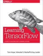
TensorFlow Serving, written in C++, is a high-performance serving framework with which we can deploy our model in a production setting. It makes our model usable for production by enabling client software to access it and pass inputs through Serving’s API (Figure 10-1). Of course, TensorFlow Serving is designed to have seamless integration with TensorFlow models. Serving features many optimizations to reduce latency and increase throughput of predictions, useful for real-time, large-scale applications. It’s not only about accessibility and efficient serving of predictions, but also about flexibility—it’s quite common to want to keep a model updated for various reasons, like having additional training data for improving the model, making changes to the network architecture, and more.

Figure 10-1. Serving links our trained model to external applications, allowing client software easy access.
Overview
Say that we run a speech-recognition service and we want to deploy our models with TensorFlow Serving. In addition to optimized serving, it is important for us to update our models periodically as we obtain more data or experiment with new network architectures. In slightly more technical terms, we’d like to have the ability to load new models and serve their outputs, and unload old ones, all while streamlining model life-cycle management and version policies.
In general terms, we can accomplish this with Serving as follows. In Python, we define the model and prepare it to be serialized in a way that can be parsed by the different modules responsible for loading, serving, and managing versions, for example. The core Serving “engine” resides in a C++ module that we will need to access only if we wish to control specific tuning and customization of Serving behaviors.
In a nutshell, this is how Serving’s architecture works (Figure 10-2):
- A module called
Sourceidentifies new models to be loaded by monitoring plugged-in filesystems, which contain our models and their associated information that we exported upon creation.Sourceincludes submodules that periodically inspect the filesystem and determine the latest relevant model versions. -
When it identifies a new model version, source creates a loader. The loader passes its servables (objects that clients use to perform computations such as predictions) to a manager. The manager handles the full life cycle of servables (loading, unloading, and serving) according to a version policy (gradual rollout, reverting versions, etc.).
- Finally, the manager provides an interface for client access to servables.

Figure 10-2. An outline of the Serving architecture.
What’s especially nice about how Serving is built is that it’s designed to be flexible and extendable. It supports building various plug-ins to customize system behavior, while using the generic builds of other core components.
In the next section we will build and deploy a TensorFlow model with Serving, demonstrating some of its key functionalities and inner workings. In advanced applications it is likely that we may have to control for different types of optimizations and customization; for example, controlling version policies and more. In this chapter we show you how to get up and running with Serving and understand its fundamentals, laying the foundations for production-ready deployment.
Installation
Serving requires several installations, including some third-party components. The installation can be done from source or using Docker, which we use here to get you started quickly. A Docker container bundles together a software application with everything needed to run it (for example, code, files, etc.). We also use Bazel, Google’s own build tool for building client and server software. In this chapter we only briefly touch on the technicalities behind tools such as Bazel and Docker. More comprehensive descriptions appear in the appendix, at the end of the book.
Installing Serving
Docker installation instructions can be found in on the Docker website.
Here, we demonstrate the Docker setup using Ubuntu.
Docker containers are created from a local Docker image, which is built from a dockerfile, and encapsulates everything we need (dependency installations, project code, etc.). Once we have Docker installed, we need to download the TensorFlow Serving dockerfile.
This dockerfile contains all of the dependencies needed to build TensorFlow Serving.
First, we produce the image from which we can run containers (this may take some time):
docker build --pull -t $USER/tensorflow-serving-devel -f
                                                  Dockerfile.devel .
Now that we’ve got the image created locally on our machine, we can create and run a container by using:
docker run -v $HOME/docker_files:/host_files
                         -p 80:80 -it $USER/tensorflow-serving-devel
The docker run -it $USER/tensorflow-serving-devel command would suffice to create and run a container, but we make two additions to this command.
First, we add -v $HOME/home_dir:/docker_dir, where -v (volume) indicates a request for a shared filesystem so we have a convenient way to transfer files between the Docker container and the host. Here we created the shared folders docker_files on our host and host_files on our Docker container. Another way to transfer files is simply by using the command docker cp foo.txt mycontainer:/foo.txt. The second addition is -p <host port>:<container port>, which makes the service in the container accessible from anywhere by having the indicated port exposed.
Once we enter our run command, a container will be created and started, and a terminal will be opened. We can have a look at our container’s status by using the command docker ps -a (outside the Docker terminal). Note that each time we use the docker run command, we create another container; to enter the terminal of an existing container, we need to use docker exec -it <container id> bash.
Finally, within the opened terminal we clone and configure TensorFlow Serving:
git clone --recurse-submodules https://github.com/tensorflow/serving
cd serving/tensorflow
./configure
And that’s it; we’re ready to go!
Building and Exporting
Now that Serving is cloned and operational, we can start exploring its features and how to use it. The cloned TensorFlow Serving libraries are organized in a Bazel architecture. The source code Bazel builds upon is organized in a workspace directory, inside nested hierarchies of packages that group related source files together. Each package has a BUILD file, specifying the output to be built from the files inside that package.
The workspace in our cloned library is located in the /serving folder, containing the WORKSPACE text file and the /tensorflow_serving package, which we will return to later.
We now turn to look at the Python script that handles the training and exportation of the model, and see how to export our model in a manner ready for serving.
Exporting our model
As when we used the Saver class, our trained model will be serialized and exported to two files: one that contains information about our variables, and another that holds information about our graph and other metadata. As we shall see shortly, Serving requires a specific serialization format and metadata, so we cannot simply use the Saver class, as we saw at the beginning of this chapter.
The steps we are going to take are as follows:
- Define our model as in previous chapters.
- Create a model builder instance.
- Have our metadata (model, method, inputs and outputs, etc.) defined in the builder in a serialized format (this is referred to as
SignatureDef). - Save our model by using the builder.
We start by creating a builder instance using Serving’s SavedModelBuilder module, passing the location to which we want our files to be exported (the directory will be created if it does not exist). SavedModelBuilder exports serialized files representing our model in the required format:
builder=saved_model_builder.SavedModelBuilder(export_path)
The serialized model files we need will be contained in a directory whose name will specify the model and its version:
export_path_base=sys.argv[-1]export_path=os.path.join(compat.as_bytes(export_path_base),compat.as_bytes(str(FLAGS.model_version)))
This way, each version will be exported to a distinct subdirectory with its corresponding path.
Note that the export_path_base is obtained as input from the command line with sys.argv, and the version is kept as a flag (presented in the previous chapter). Flag parsing is handled by tf.app.run(), as we will see shortly.
Next, we want to define the input (shape of the input tensor of the graph) and output (tensor of the prediction) signatures. In the first part of this chapter we used TensorFlow collection objects to specify the relation between input and output data and their corresponding placeholders, and also operations for computing predictions and accuracy. Here, signatures serve a somewhat analogous purpose.
We use the builder instance we created to add both the variables and meta graph information, using the SavedModelBuilder.add_meta_graph_and_variables() method:
builder.add_meta_graph_and_variables(sess,[tag_constants.SERVING],signature_def_map={'predict_images':prediction_signature,signature_constants.DEFAULT_SERVING_SIGNATURE_DEF_KEY:classification_signature,},legacy_init_op=legacy_init_op)
We need to pass four arguments: the session, tags (to “serve” or “train”), the signature map, and some initializations.
We pass a dictionary with the prediction and classification signatures. We start with the prediction signature, which again can be thought of as analogical to specifying and saving a prediction op in a TensorFlow collection as we saw earlier:
prediction_signature=signature_def_utils.build_signature_def(inputs={'images':tensor_info_x},outputs={'scores':tensor_info_y},method_name=signature_constants.PREDICT_METHOD_NAME)
images and scores here are arbitrary names that we will use to refer to our x and y Tensors later. The images and scores are encoded into the required format by using the following commands:
tensor_info_x=utils.build_tensor_info(x)tensor_info_y=utils.build_tensor_info(y_conv)
Similar to the prediction signature, we have the classification signature, where we input the information about the scores (the probability values of the top k classes) and the corresponding classes:
# Build the signature_def_mapclassification_inputs=utils.build_tensor_info(serialized_tf_example)classification_outputs_classes=utils.build_tensor_info(prediction_classes)classification_outputs_scores=utils.build_tensor_info(values)
classification_signature=signature_def_utils.build_signature_def(inputs={signature_constants.CLASSIFY_INPUTS:classification_inputs},outputs={signature_constants.CLASSIFY_OUTPUT_CLASSES:classification_outputs_classes,signature_constants.CLASSIFY_OUTPUT_SCORES:classification_outputs_scores},method_name=signature_constants.CLASSIFY_METHOD_NAME)
Finally, we save our model by using the save() command:
builder.save()
This, in a nutshell, wraps all the parts together in a format ready to be serialized and exported upon execution of the script, as we shall see immediately.
Here is the final code for our main Python model script, including our model (the CNN model from Chapter 4):
importosimportsysimporttensorflowastffromtensorflow.python.saved_modelimportbuilderassaved_model_builderfromtensorflow.python.saved_modelimportsignature_constantsfromtensorflow.python.saved_modelimportsignature_def_utilsfromtensorflow.python.saved_modelimporttag_constantsfromtensorflow.python.saved_modelimportutilsfromtensorflow.python.utilimportcompatfromtensorflow_serving.exampleimportmnist_input_datatf.app.flags.DEFINE_integer('training_iteration',10,'number of training iterations.')tf.app.flags.DEFINE_integer('model_version',1,'version number of the model.')tf.app.flags.DEFINE_string('work_dir','/tmp','Working directory.')FLAGS=tf.app.flags.FLAGSdefweight_variable(shape):initial=tf.truncated_normal(shape,stddev=0.1)returntf.Variable(initial,dtype='float')defbias_variable(shape):initial=tf.constant(0.1,shape=shape)returntf.Variable(initial,dtype='float')defconv2d(x,W):returntf.nn.conv2d(x,W,strides=[1,1,1,1],padding='SAME')defmax_pool_2x2(x):returntf.nn.max_pool(x,ksize=[1,2,2,1],strides=[1,2,2,1],padding='SAME')defmain(_):iflen(sys.argv)<2orsys.argv[-1].startswith('-'):('Usage: mnist_export.py [--training_iteration=x] ''[--model_version=y] export_dir')sys.exit(-1)ifFLAGS.training_iteration<=0:('Please specify a positivevaluefortrainingiteration.')sys.exit(-1)ifFLAGS.model_version<=0:('Please specify a positivevalueforversionnumber.')sys.exit(-1)('Training...')mnist=mnist_input_data.read_data_sets(FLAGS.work_dir,one_hot=True)sess=tf.InteractiveSession()serialized_tf_example=tf.placeholder(tf.string,name='tf_example')feature_configs={'x':tf.FixedLenFeature(shape=[784],dtype=tf.float32),}tf_example=tf.parse_example(serialized_tf_example,feature_configs)x=tf.identity(tf_example['x'],name='x')y_=tf.placeholder('float',shape=[None,10])W_conv1=weight_variable([5,5,1,32])b_conv1=bias_variable([32])x_image=tf.reshape(x,[-1,28,28,1])h_conv1=tf.nn.relu(conv2d(x_image,W_conv1)+b_conv1)h_pool1=max_pool_2x2(h_conv1)W_conv2=weight_variable([5,5,32,64])b_conv2=bias_variable([64])h_conv2=tf.nn.relu(conv2d(h_pool1,W_conv2)+b_conv2)h_pool2=max_pool_2x2(h_conv2)W_fc1=weight_variable([7*7*64,1024])b_fc1=bias_variable([1024])h_pool2_flat=tf.reshape(h_pool2,[-1,7*7*64])h_fc1=tf.nn.relu(tf.matmul(h_pool2_flat,W_fc1)+b_fc1)keep_prob=tf.placeholder(tf.float32)h_fc1_drop=tf.nn.dropout(h_fc1,keep_prob)W_fc2=weight_variable([1024,10])b_fc2=bias_variable([10])y_conv=tf.matmul(h_fc1_drop,W_fc2)+b_fc2y=tf.nn.softmax(y_conv,name='y')cross_entropy=-tf.reduce_sum(y_*tf.log(y_conv))train_step=tf.train.AdamOptimizer(1e-4).minimize(cross_entropy)values,indices=tf.nn.top_k(y_conv,10)prediction_classes=tf.contrib.lookup.index_to_string(tf.to_int64(indices),mapping=tf.constant([str(i)foriinxrange(10)]))sess.run(tf.global_variables_initializer())for_inrange(FLAGS.training_iteration):batch=mnist.train.next_batch(50)train_step.run(feed_dict={x:batch[0],y_:batch[1],keep_prob:0.5})(_)correct_prediction=tf.equal(tf.argmax(y_conv,1),tf.argmax(y_,1))accuracy=tf.reduce_mean(tf.cast(correct_prediction,'float'))y_:mnist.test.labels})('training accuracy%g'%accuracy.eval(feed_dict={x:mnist.test.images,y_:mnist.test.labels,keep_prob:1.0}))('training is finished!')export_path_base=sys.argv[-1]export_path=os.path.join(compat.as_bytes(export_path_base),compat.as_bytes(str(FLAGS.model_version)))'Exporting trained model to',export_pathbuilder=saved_model_builder.SavedModelBuilder(export_path)classification_inputs=utils.build_tensor_info(serialized_tf_example)classification_outputs_classes=utils.build_tensor_info(prediction_classes)classification_outputs_scores=utils.build_tensor_info(values)classification_signature=signature_def_utils.build_signature_def(inputs={signature_constants.CLASSIFY_INPUTS:classification_inputs},outputs={signature_constants.CLASSIFY_OUTPUT_CLASSES:classification_outputs_classes,signature_constants.CLASSIFY_OUTPUT_SCORES:classification_outputs_scores},method_name=signature_constants.CLASSIFY_METHOD_NAME)tensor_info_x=utils.build_tensor_info(x)tensor_info_y=utils.build_tensor_info(y_conv)prediction_signature=signature_def_utils.build_signature_def(inputs={'images':tensor_info_x},outputs={'scores':tensor_info_y},method_name=signature_constants.PREDICT_METHOD_NAME)legacy_init_op=tf.group(tf.initialize_all_tables(),name='legacy_init_op')builder.add_meta_graph_and_variables(sess,[tag_constants.SERVING],signature_def_map={'predict_images':prediction_signature,signature_constants.DEFAULT_SERVING_SIGNATURE_DEF_KEY:classification_signature,},legacy_init_op=legacy_init_op)builder.save()('new model exported!')if__name__=='__main__':tf.app.run()
The tf.app.run() command gives us a nice wrapper that handles parsing command-line arguments.
In the final part of our introduction to Serving, we use Bazel for the actual exporting and deployment of our model.
Most Bazel BUILD files consist only of declarations of build rules specifying the relationship between inputs and outputs, and the steps to build the outputs.
For instance, in this BUILD file we have a Python rule py_binary to build executable programs. Here we have three attributes, name for the name of the rule, srcs for the list of files that are processed to create the target (our Python script), and deps for the list of other libraries to be linked into the binary target:
py_binary(
    name = "serving_model_ch4",
    srcs = [
        "serving_model_ch4.py",
    ],
    deps = [
        ":mnist_input_data",
        "@org_tensorflow//tensorflow:tensorflow_py",
        "@org_tensorflow//tensorflow/python/saved_model:builder",
        "@org_tensorflow//tensorflow/python/saved_model:constants",
        "@org_tensorflow//tensorflow/python/saved_model:loader",
        "@org_tensorflow//tensorflow/python/saved_model:
                                              signature_constants",
        "@org_tensorflow//tensorflow/python/saved_model:
                                              signature_def_utils",
        "@org_tensorflow//tensorflow/python/saved_model:
                                              tag_constants",
        "@org_tensorflow//tensorflow/python/saved_model:utils",
    ],
)
Next we run and export the model by using Bazel, training with 1,000 iterations and exporting the first version of the model:
bazel build //tensorflow_serving/example:serving_model_ch4
bazel-bin/tensorflow_serving/example/serving_model_ch4
        --training_iteration=1000 --model_version=1 /tmp/mnist_model
To train the second version of the model, we just use:
--model_version=2
In the designated subdirectory we will find two files, saved_model.pb and variables, that contain the serialized information about our graph (including metadata) and its variables, respectively. In the next lines we load the exported model with the standard TensorFlow model server:
bazel build //tensorflow_serving/model_servers:
                                           tensorflow_model_server
bazel-bin/tensorflow_serving/model_servers/tensorflow_model_server
                  --port=8000 --model_name=mnist
                  --model_base_path=/tmp/mnist_model/ --logtostderr
Finally, our model is now served and ready for action at localhost:8000. We can test the server with a simple client utility, mnist_client:
bazel build //tensorflow_serving/example:mnist_client
bazel-bin/tensorflow_serving/example/mnist_client
                          --num_tests=1000 --server=localhost:8000
Summary
This chapter dealt with how to save, export, and serve models, from simply saving and reassigning of weights using the built-in Saver utility to an advanced model-deployment mechanism for production. The last part of this chapter touched on TensorFlow Serving, a great tool for making our models commercial-ready with dynamic version control. Serving is a rich utility with many functionalities, and we strongly recommend that readers who are interested in mastering it seek out more in-depth technical material online.