Installing TensorFlow

If you are using a clean Python installation (probably set up for the purpose of learning TensorFlow), you can get started with the simple pip installation:

$ pip install tensorflow

This approach does, however, have the drawback that TensorFlow will override existing packages and install specific versions to satisfy dependencies. If you are using this Python installation for other purposes as well, this will not do. One common way around this is to install TensorFlow in a virtual environment, managed by a utility called virtualenv.

Depending on your setup, you may or may not need to install virtualenv on your machine. To install virtualenv, type:

$ pip install virtualenv

See http://virtualenv.pypa.io for further instructions.

In order to install TensorFlow in a virtual environment, you must first create the virtual environment—in this book we choose to place these in the ~/envs folder, but feel free to put them anywhere you prefer:

$ cd ~
$ mkdir envs
$ virtualenv ~/envs/tensorflow

This will create a virtual environment named tensorflow in ~/envs (which will manifest as the folder ~/envs/tensorflow). To activate the environment, use:

$ source ~/envs/tensorflow/bin/activate

The prompt should now change to indicate the activated environment:

(tensorflow)$

At this point the pip install command:

(tensorflow)$ pip install tensorflow​

will install TensorFlow into the virtual environment, without impacting other packages installed on your machine.

Finally, in order to exit the virtual environment, you type:

(tensorflow)$ deactivate

at which point you should get back the regular prompt:

$

alias tensorflow="source ~/envs/tensorflow/bin/activate"

Now that we have a basic installation of TensorFlow, we can proceed to our first working examples. We will follow the well-established tradition and start with a “hello world” program.

Hello World

Our first example is a simple program that combines the words “Hello” and “ World!” and displays the output—the phrase “Hello World!” While simple and straightforward, this example introduces many of the core elements of TensorFlow and the ways in which it is different from a regular Python program.

We suggest you run this example on your machine, play around with it a bit, and see what works. Next, we will go over the lines of code and discuss each element separately.

First, we run a simple install and version check (if you used the virtualenv installation option, make sure to activate it before running TensorFlow code):

import tensorflow as tf
print(tf.__version__)

If correct, the output will be the version of TensorFlow you have installed on your system. Version mismatches are the most probable cause of issues down the line.

Example 2-1 shows the complete “hello world” example.

import tensorflow as tf

h = tf.constant("Hello")
w = tf.constant(" World!")
hw = h + w

with tf.Session() as sess:
    ans = sess.run(hw)

print (ans)

We assume you are familiar with Python and imports, in which case the first line:

import tensorflow as tf

requires no explanation.

Next, we define the constants "Hello" and " World!", and combine them:

import tensorflow as tf

h = tf.constant("Hello")
w = tf.constant(" World!")
hw = h + w 

At this point, you might wonder how (if at all) this is different from the simple Python code for doing this:

ph = "Hello"
pw = " World!"
phw = h + w

The key point here is what the variable hw contains in each case. We can check this using the print command. In the pure Python case we get this:

>print phw
Hello World!

In the TensorFlow case, however, the output is completely different:

>print hw
Tensor("add:0", shape=(), dtype=string)

Probably not what you expected!

In the next chapter we explain the computation graph model of TensorFlow in detail, at which point this output will become completely clear. The key idea behind computation graphs in TensorFlow is that we first define what computations should take place, and then trigger the computation in an external mechanism. Thus, the TensorFlow line of code:

hw = h + w 

does not compute the sum of h and w, but rather adds the summation operation to a graph of computations to be done later.

Next, the Session object acts as an interface to the external TensorFlow computation mechanism, and allows us to run parts of the computation graph we have already defined. The line:

ans = sess.run(hw)

actually computes hw (as the sum of h and w, the way it was defined previously), following which the printing of ans displays the expected “Hello World!” message.

This completes the first TensorFlow example. Next, we dive right in with a simple machine learning example, which already shows a great deal of the promise of the TensorFlow framework.

MNIST

The MNIST (Mixed National Institute of Standards and Technology) handwritten digits dataset is one of the most researched datasets in image processing and machine learning, and has played an important role in the development of artificial neural networks (now generally referred to as deep learning).

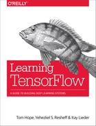
As such, it is fitting that our first machine learning example should be dedicated to the classification of handwritten digits (Figure 2-1 shows a random sample from the dataset). At this point, in the interest of keeping it simple, we will apply a very simple classifier. This simple model will suffice to classify approximately 92% of the test set correctly—the best models currently available reach over 99.75% correct classification, but we have a few more chapters to go until we get there! Later in the book, we will revisit this data and use more sophisticated methods.

Figure 2-1. 100 random MNIST images

Softmax Regression

In this example we will use a simple classifier called softmax regression. We will not go into the mathematical formulation of the model in too much detail (there are plenty of good resources where you can find this information, and we strongly suggest that you do so, if you have never seen this before). Rather, we will try to provide some intuition into the way the model is able to solve the digit recognition problem.

Put simply, the softmax regression model will figure out, for each pixel in the image, which digits tend to have high (or low) values in that location. For instance, the center of the image will tend to be white for zeros, but black for sixes. Thus, a black pixel in the center of an image will be evidence against the image containing a zero, and in favor of it containing a six.

Learning in this model consists of finding weights that tell us how to accumulate evidence for the existence of each of the digits. With softmax regression, we will not use the spatial information in the pixel layout in the image. Later on, when we discuss convolutional neural networks, we will see that utilizing spatial information is one of the key elements in making great image-processing and object-recognition models.

Since we are not going to use the spatial information at this point, we will unroll our image pixels as a single long vector denoted x (Figure 2-2). Then

xw⁰ = ∑x_i$w_i^0$

will be the evidence for the image containing the digit 0 (and in the same way we will have $w^d$ weight vectors for each one of the other digits, $d=1,...,9$).

Figure 2-2. MNIST image pixels unrolled to vectors and stacked as columns (sorted by digit from left to right). While the loss of spatial information doesn’t allow us to recognize the digits, the block structure evident in this figure is what allows the softmax model to classify images. Essentially, all zeros (leftmost block) share a similar pixel structure, as do all ones (second block from the left), etc.

All this means is that we sum up the pixel values, each multiplied by a weight, which we think of as the importance of this pixel in the overall evidence for the digit zero being in the image.²

For instance, w⁰₃₈ will be a large positive number if the 38th pixel having a high intensity points strongly to the digit being a zero, a strong negative number if high-intensity values in this position occur mostly in other digits, and zero if the intensity value of the 38th pixel tells us nothing about whether or not this digit is a zero.³

Performing this calculation at once for all digits (computing the evidence for each of the digits appearing in the image) can be represented by a single matrix operation. If we place the weights for each of the digits in the columns of a matrix W, then the length-10 vector with the evidence for each of the digits is

[xw⁰, ···, xw⁹] = xW

The purpose of learning a classifier is almost always to evaluate new examples. In this case, this means that we would like to be able to tell what digit is written in a new image we have not seen in our training data. In order to do this, we start by summing up the evidence for each of the 10 possible digits (i.e., computing xW). The final assignment will be the digit that “wins” by accumulating the most evidence:

digit = argmax(xW)

We start by presenting the code for this example in its entirety (Example 2-2), then walk through it line by line and go over the details. You may find that there are many novel elements or that some pieces of the puzzle are missing at this stage, but our advice is that you go with it for now. Everything will become clear in due course.

import tensorflow as tf
from tensorflow.examples.tutorials.mnist import input_data


DATA_DIR = '/tmp/data'
NUM_STEPS = 1000
MINIBATCH_SIZE = 100


data = input_data.read_data_sets(DATA_DIR, one_hot=True)

x = tf.placeholder(tf.float32, [None, 784])
W = tf.Variable(tf.zeros([784, 10]))

y_true = tf.placeholder(tf.float32, [None, 10])
y_pred = tf.matmul(x, W)

cross_entropy = tf.reduce_mean(tf.nn.softmax_cross_entropy_with_logits(
    logits=y_pred, labels=y_true))


gd_step = tf.train.GradientDescentOptimizer(0.5).minimize(cross_entropy)

correct_mask = tf.equal(tf.argmax(y_pred, 1), tf.argmax(y_true, 1))
accuracy = tf.reduce_mean(tf.cast(correct_mask, tf.float32))

with tf.Session() as sess:

    # Train
    sess.run(tf.global_variables_initializer())

    for _ in range(NUM_STEPS):
        batch_xs, batch_ys = data.train.next_batch(MINIBATCH_SIZE)
        sess.run(gd_step, feed_dict={x: batch_xs, y_true: batch_ys})

    # Test
    ans = sess.run(accuracy, feed_dict={x: data.test.images, 
                                        y_true: data.test.labels})

print "Accuracy: {:.4}%".format(ans*100)

If you run the code on your machine, you should get output like this:

Extracting /tmp/data/train-images-idx3-ubyte.gz
Extracting /tmp/data/train-labels-idx1-ubyte.gz
Extracting /tmp/data/t10k-images-idx3-ubyte.gz
Extracting /tmp/data/t10k-labels-idx1-ubyte.gz
Accuracy: 91.83%

That’s all it takes! If you have put similar models together before using other platforms, you might appreciate the simplicity and readability. However, these are just side bonuses, with the efficiency and flexibility gained from the computation graph model of TensorFlow being what we are really interested in.

The exact accuracy value you get will be just under 92%. If you run the program once more, you will get another value. This sort of stochasticity is very common in machine learning code, and you have probably seen similar results before. In this case, the source is the changing order in which the handwritten digits are presented to the model during learning. As a result, the learned parameters following training are slightly different from run to run.

Running the same program five times might therefore produce this result:

Accuracy: 91.86%
Accuracy: 91.51%
Accuracy: 91.62%
Accuracy: 91.93%
Accuracy: 91.88%

We will now briefly go over the code for this example and see what is new from the previous “hello world” example. We’ll break it down line by line:

import tensorflow as tf
from tensorflow.examples.tutorials.mnist import input_data

The first new element in this example is that we use external data! Rather than downloading the MNIST dataset (freely available at http://yann.lecun.com/exdb/mnist/) and loading it into our program, we use a built-in utility for retrieving the dataset on the fly. Such utilities exist for most popular datasets, and when dealing with small ones (in this case only a few MB), it makes a lot of sense to do it this way. The second import loads the utility we will later use both to automatically download the data for us, and to manage and partition it as needed:

DATA_DIR = '/tmp/data'
NUM_STEPS = 1000
MINIBATCH_SIZE = 100

Here we define some constants that we use in our program—these will each be explained in the context in which they are first used:

data = input_data.read_data_sets(DATA_DIR, one_hot=True)

The read_data_sets() method of the MNIST reading utility downloads the dataset and saves it locally, setting the stage for further use later in the program. The first argument, DATA_DIR, is the location we wish the data to be saved to locally. We set this to '/tmp/data', but any other location would be just as good. The second argument tells the utility how we want the data to be labeled; we will not go into this right now.⁴

Note that this is what prints the first four lines of the output, indicating the data was obtained correctly. Now we are finally ready to set up our model:

x = tf.placeholder(tf.float32, [None, 784])
W = tf.Variable(tf.zeros([784, 10]))

In the previous example we saw the TensorFlow constant element—this is now complemented by the placeholder and Variable elements. For now, it is enough to know that a variable is an element manipulated by the computation, while a placeholder has to be supplied when triggering it. The image itself (x) is a placeholder, because it will be supplied by us when running the computation graph. The size [None, 784] means that each image is of size 784 (28×28 pixels unrolled into a single vector), and None is an indicator that we are not currently specifying how many of these images we will use at once:

y_true = tf.placeholder(tf.float32, [None, 10])
y_pred = tf.matmul(x, W)

In the next chapter these concepts will be dealt with in much more depth.

A key concept in a large class of machine learning tasks is that we would like to learn a function from data examples (in our case, digit images) to their known labels (the identity of the digit in the image). This setting is called supervised learning. In most supervised learning models, we attempt to learn a model such that the true labels and the predicted labels are close in some sense. Here, y_true and y_pred are the elements representing the true and predicted labels, respectively:

cross_entropy = tf.reduce_mean(tf.nn.softmax_cross_entropy_with_logits(
    logits=y_pred, labels=y_true))

The measure of similarity we choose for this model is what is known as cross entropy—a natural choice when the model outputs class probabilities. This element is often referred to as the loss function:⁵

gd_step = tf.train.GradientDescentOptimizer(0.5).minimize(cross_entropy)

The final piece of the model is how we are going to train it (i.e., how we are going to minimize the loss function). A very common approach is to use gradient descent optimization. Here, 0.5 is the learning rate, controlling how fast our gradient descent optimizer shifts model weights to reduce overall loss.

We will discuss optimizers and how they fit into the computation graph later on in the book.

Once we have defined our model, we want to define the evaluation procedure we will use in order to test the accuracy of the model. In this case, we are interested in the fraction of test examples that are correctly classified:⁶

correct_mask = tf.equal(tf.argmax(y_pred, 1), tf.argmax(y_true, 1))
accuracy = tf.reduce_mean(tf.cast(correct_mask, tf.float32)) 

As with the “hello world” example, in order to make use of the computation graph we defined, we must create a session. The rest happens within the session:

with tf.Session() as sess:

First, we must initialize all variables:

    sess.run(tf.global_variables_initializer())

This carries some specific implications in the realm of machine learning and optimization, which we will discuss further when we use models for which initialization is an important issue

    for _ in range(NUM_STEPS):
        batch_xs, batch_ys = data.train.next_batch(MINIBATCH_SIZE)
        sess.run(gd_step, feed_dict={x: batch_xs, y_true: batch_ys})

The actual training of the model, in the gradient descent approach, consists of taking many steps in “the right direction.” The number of steps we will make, NUM_STEPS, was set to 1,000 in this case. There are more sophisticated ways of deciding when to stop, but more about that later! In each step we ask our data manager for a bunch of examples with their labels and present them to the learner. The MINIBATCH_SIZE constant controls the number of examples to use for each step.

Finally, we use the feed_dict argument of sess.run for the first time. Recall that we defined placeholder elements when constructing the model. Now, each time we want to run a computation that will include these elements, we must supply a value for them.

    ans = sess.run(accuracy, feed_dict={x: data.test.images,
                                        y_true: data.test.labels})

In order to evaluate the model we have just finished learning, we run the accuracy computing operation defined earlier (recall the accuracy was defined as the fraction of images that are correctly labeled). In this procedure, we feed a separate group of test images, which were never seen by the model during training:

    print "Accuracy: {:.4}%".format(ans*100)

Lastly, we print out the results as percent values.

Figure 2-3 shows a graph representation of our model.

Figure 2-3. A graph representation of the model. Rectangular elements are Variables, and circles are placeholders. The top-left frame represents the label prediction part, and the bottom-right frame the evaluation. Here, b is a bias term that could be added to the mode.

feed_dict={x: data.test.images, y_true: data.test.labels}
ans = sess.run(accuracy, feed_dict)

Summary

Congratulations! By now you have installed TensorFlow and taken it for a spin with two basic examples. You have seen some of the fundamental building blocks that will be used throughout the book, and have hopefully begun to get a feel for TensorFlow.

Next, we take a look under the hood and explore the computation graph model used by TensorFlow.