
Chapter 2
Dynamic Security Design and Corporate Financing*
Abstract
Keywords
Security design; Dynamic contracts; Moral hazard; Asymmetric information; Signaling; Incentives
1 Introduction
Modigliani and Miller (1958), hereafter MM, argue that under certain idealized assumptions firm capital structure is irrelevant, i.e. it does not affect firm value. These conditions include:
1. There are no taxes or bankruptcy costs.
2. There are no agency problems.
3. There are no differences in information between insiders and outside investors.
4. Capital markets are frictionless, i.e. market participants are perfectly competitive and have no market power, and there is no security mispricing.
Of course, we know that these idealized conditions clearly fail in practice. The important message of the Modigliani–Miller theory is that it rules out certain commonly used arguments about capital structure as incorrect or incomplete. These arguments typically fail to take into account that the riskiness of securities used in capital structure, and thus their required return, depend on the capital structure itself. Here are some typical examples:
A. An argument against higher capital requirements for banks: because equity has a higher required return than debt, requiring banks to hold more equity in their capital structure to absorb risk will make banks less profitable. This argument fails to take into account that a decrease in leverage makes equity less risky, and thus lowers the cost of equity.1
B. An argument that calls on technology firms, such as Apple, to pay out their cash holdings, because cash earns a much lower rate of return than these firms’ cost of capital. This argument fails to take into account that cash is less risky than the rest of the firm and so the required return on cash is significantly lower than the cost of equity.
C. An argument that merging firms can create value for their shareholders through “corporate diversification”. This argument ignores that shareholders can diversify themselves.
Of course, there are valid contributions to these debates that are based on the violations of Modigliani–Miller conditions. These focus on the relationship between leverage/cash holdings and incentives, distinctions between inside and outside equity, and bankruptcy costs. This essay explores the implications of these frictions on capital structure.
The Modigliani–Miller Propositions. Consider a firm that generates a random stream of cash flows:
![]()
at time points 1, 2, etc. Firm capital structure divides these cash flows between debt holders and equity holders, and possibly other security holders, in some way. According to MM, the value of the firm does not depend on how these cash flows are divided among the firm’s stake holders. Behind this result is the principle of arbitrage. Using frictionless financial markets, participants should be able to replicate the payoff of any structured security backed by the firm’s cash flows, with zero transaction costs and zero market impact.
The most basic example that illustrates the MM propositions involves a one-period firm that generates a single random cash flow of ![]() at date 1. Suppose that the firm has debt with face value D and the risk-free interest rate is r. Then at date 1, debt holders get (1 + r)D and equity holders get
at date 1. Suppose that the firm has debt with face value D and the risk-free interest rate is r. Then at date 1, debt holders get (1 + r)D and equity holders get ![]() , assuming that
, assuming that ![]() is always large enough to make debt risk-free. Denote by E the market value of this firm’s equity.
is always large enough to make debt risk-free. Denote by E the market value of this firm’s equity.
MM Proposition 1
Assume that there is an identical all-equity firm 2, with value V. That is, firm 2 also generates a cash flow of![]() at date 1. Then:
at date 1. Then:
![]()
That is, the two firms with different capital structure but the same cash flows have the same value.
Proof.
The proof uses the principle of arbitrage.
If D + E > V, consider selling short a fraction α > 0 of equity of firm 1, borrowing αD, and using αV < αE + αD of the proceeds to buy a fraction α of firm 2. This position can be liquidated at no cost at date 1, since the proceeds ![]() from the stake in firm 2 are just sufficient to repurchase equity of firm 1 for
from the stake in firm 2 are just sufficient to repurchase equity of firm 1 for ![]() and have
and have ![]() left to pay down debt. At the same time, this trading strategy generates an instantaneous profit of αE + αD − αV at date 0. That is, if D + E > V than there is an arbitrage opportunity.
left to pay down debt. At the same time, this trading strategy generates an instantaneous profit of αE + αD − αV at date 0. That is, if D + E > V than there is an arbitrage opportunity.
If D + E < V then this strategy can be executed in reverse to generate an instant profit of αV − αE − αD.
MM Proposition 2 derives how the required return on the firm’s equity changes with capital structure. Let ![]() and denote by:
and denote by:
![]()
the req uired rate of return on the firm’s assets.
MM Proposition 2
The required rate of return on the firm’s equity, ![]() , satisfies
, satisfies
![]()
This proposition implies that, if firm investors require compensation for the firm’s risk, that is, rA > r, then as firm leverage D/E increases, the cost of equity rE increases. That is, as equity becomes riskier with greater leverage, equity holders require a higher compensation for risk.
MM Proposition 2 is related to example A about the amount of equity that banks are required to hold to absorb losses. Under MM assumptions, higher capital requirements would not make banks less profitable because lower leverage would lead to a lower cost of equity. Of course, violations of the MM assumptions immediately enter the debate. A key counterargument is that debt has a tax advantage, and thus leverage can reduce the cost of capital.
The focus of this essay is the relationship between information and capital structure. Insiders, e.g. firm managers, may have information about firm fundamentals that the market does not know. There may also be a conflict of interest, i.e. agency problems, between firm insiders and outside investors. Models of these informational problems predict a specific division of cash flows between insiders and outsiders. A typical result is that insiders must hold an equity-like security backed by the firm’s assets. Such a security allows insiders to signal good information about firm fundamentals in settings with adverse selection, and it gives insiders incentives to take actions that increase firm value in settings of moral hazard.
While models of agency problems and asymmetric information have very clear implications on the division of cash flows between insiders and outsiders, they typically say very little about the division of cash flows among outsiders. Trade-off theory models, such as that of Leland (1994), explore the optimal division of firm cash flows between outside debt and equity holders taking into account tax advantages of debt and bankruptcy costs.
The rest of the essay is organized as follows. In Section 2 we review theories of capital structure based on static models of informational asymmetries. In Section 3 we move on to a dynamic environment based on the model of Leland (1994), in which we explore trade-offs between bankruptcy costs and tax advantages of debt, and incentive properties of simple contracts. In Section 4 we explore the full-blown problem of optimal contracts in dynamic moral hazard environments. In Section 5 we explore dynamic adverse selection and market dynamics.
2 Informational Problems in Static Models
In this section we explore static models of informational problems. One classic early reference on capital structure and the scope of the firm in the presence of agency models is Jensen and Meckling (1976). If a firm manager is risk-neutral, then a 100% managerial equity stake in the firm leads to an efficient outcome. The manager will then take actions that maximize the shareholder value of the firm (which includes the value of non-pecuniary benefits that the manager receives). Moreover, if the manager has private information about firm fundamentals, he does not have any incentive to misrepresent it to the market.
If the manager is risk-averse, then the optimal security design problem becomes nontrivial. The most rudimentary way to capture risk-aversion in a model is by imposing a limited liability constraint—the manager cannot consume negative amounts, and a more general way is by assuming a concave utility function. If so, then it may be necessary and beneficial for the manager to sell some of his equity stake, or another security backed by the firm’s assets, to raise funding for the firm. Selling securities to raise funds can lead to various inefficiencies: reducing the manager’s effort, requiring costly monitoring actions or inefficient project liquidation. It may also be difficult to sell securities due to informational asymmetries. In this section we explore various static models where this happens.
2.1 Moral Hazard
Townsend (1979): Townsend’s costly state verification model, which has been adapted to finance settings by Gale and Hellwig (1985), has been used widely in applications, including macro economics in work of Bernanke and Gertler (1989) and Bernanke, Gertler, and Gilchrist (1999). The costly state verification model captures deadweight costs that outside investors might need to incur to monitor the manager. A monitoring action can be required because the manager privately observes the firm’s profits, which he may divert and refuse to pay back to investors.
Consider an agent with a profitable project, which needs an investment of I > 0. The agent does not have the full amount to invest, and needs to raise some money from an outside investor, the principal.
If the investment is made, the project has a random gross return ![]() , distributed on
, distributed on ![]() with CDF F. Only the agent observes the true returns. However, the principal can verify returns at a cost c. Both the agent and the principal are risk-neutral, but the agent has limited liability—he cannot be forced to pay back more than what he claims to have, or more than what he actually has if verification takes place. An optimal contract maximizes the principal’s profit subject to giving the agent a specific expected gross payoff of W0. The value of W0 depends on the agent’s contribution towards the up-front investment, and the relative bargaining powers of the principal and the agent. Assuming that the principal must contribute a strictly positive amount to up-front investment,
with CDF F. Only the agent observes the true returns. However, the principal can verify returns at a cost c. Both the agent and the principal are risk-neutral, but the agent has limited liability—he cannot be forced to pay back more than what he claims to have, or more than what he actually has if verification takes place. An optimal contract maximizes the principal’s profit subject to giving the agent a specific expected gross payoff of W0. The value of W0 depends on the agent’s contribution towards the up-front investment, and the relative bargaining powers of the principal and the agent. Assuming that the principal must contribute a strictly positive amount to up-front investment, ![]() .
.
Assuming that the principal can perfectly commit to any contract, we can use the revelation principle to consider only truth-telling contracts, in which the agent directly reports realized output (see Myerson, 1979). We can focus on contracts {V, g(x)}, where V ⊆ [0, X] is the set of reports that the principal commits to verify, and g(x) ≤ x is a transfer that the agent is required to make if he reports x and is not caught lying. If the agent is caught lying then without loss of generality we assume that the principal takes away the agent’s entire output. This transfer rule off the equilibrium path gives the agent the maximal incentive to tell the truth.
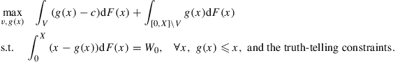
In this notation, the optimal contracting problem is written as follows:
The truth-telling constraints require that the agent be at least as well-off telling the truth rather than lying, after any output realization. Rather than writing out all truth-telling constraints explicitly, we provide a lemma that characterizes the set of all contracts that satisfy the truth-telling constraints.
Lemma 1
A feasible contract satisfies the truth-telling constraints if and only if for some constant D:
Proof
(⇒) If the agent chooses to report in the non-verification region, he will choose a report that involves the smallest transfer. Therefore, if (A) fails, it is not incentive-compatible to tell the truth in the non-verification region. Similarly, if (B) fails, then there is x ∈ V with g(x) > D. But then the agent would prefer to report something in the non-verification region than to report x. We conclude that A and B must hold in a truth-telling contract.
(⇐) If x ∈ V, then the agent weakly prefers to tell the truth and pay a transfer of g(x) rather than announce something outside V and pay D or announce something else in V and pay x. If x is outside V, then the agent is indifferent among all announcements that do not trigger verification, but weakly prefers them to any announcement that does lead to verification. Hence, truth-telling incentives hold.
The following theorem solves for the optimal contract, and shows that it takes the form of debt.
Theorem 1
The optimal contract is a standard debt contract, as illustrated inFigure 1, i.e. ∃ D s.t.

Figure 1 Function g(x) and the verification region in the standard debt contract.
Proof
Since the contract must satisfy the truth-telling constraints, there exists D such that g(x) ≤ D for x ∈ V and g(x) = D for x outside V. Then, by the feasibility constraints, the entire interval [0, D) must be a subset of V.
If we have a contract that does not satisfy the conditions outlined in Theorem 1, as illustrated on the left panel of Figure 2, we can strictly improve it in two steps. First, as illustrated on the middle panel, let us (1) move all points in V ∩ [D, X] to the non-verification region, (2) raise g(x) to D on V ∩ [D, X], and (3) raise g(x) to x on [0, D). Then the new contract satisfies the truth-telling constraints and generates higher total surplus (sum of the principal’s and agent’s payoffs), but it generates a strictly lower payoff than W0 to the agent. We then transfer value from the principal to agent, and improve surplus further, by lowering D in the second step (as shown in the right panel of Figure 2), to the point where the agent’s expected payoff equals exactly W0

Figure 2 The proof of Theorem 1.
Remark 1
A moral hazard problem exists when the agent can take an action that yields him private benefit and at the same time reduces the overall value of the project. In this setting, such an action is hiding output. A solution to a moral hazard problem requires the agent to hold some type of equity-like security. Such a security prevents the agent from taking at least some actions that are detrimental to the overall value of the project. In this setting, the agent’s security is equity in the non-verification region, i.e. he gets a marginal payoff of 1 for each incremental dollar of cash flows.
Remark 2
We assumed that only deterministic verification is allowed. If the principal could commit to stochastic verification, he could design a better contract.
Remark 3
We assumed that the principal can fully commit to any contract. This assumption provides a useful benchmark for the analysis of contracting problems. The assumption of commitment can be relaxed. In this setting, if the principal cannot commit to verify the agent, we can instead consider contracts in which the principal can have a right, but not an obligation, to verify. Under this alternative assumption, the revelation principle no longer holds but an equally efficient outcome may be attained under additional conditions.
Remark 4
The moral hazard problem has implications on the optimal amount of investment and the scale of the firm. Generally, the optimal scale rises with the amount of wealth that the agent is able to contribute into the project. In the following example, the project is infeasible if the agent cannot contribute towards up-front investment. If the agent can contribute an amount E > 0, the optimal scale rises linearly in E.
Consider a scalable project, which generates a cash flow uniformly distributed on [0, 3I] when an investment of I is made. Cash flows can be verified at the cost of cI, where ![]() . Then the principal’s payoff as a function of D is:
. Then the principal’s payoff as a function of D is:
![]()
The debt face value that maximizes this expression is D = (3 − c)I, and so the principal’s maximal payoff is (3 − c)2I/6. Consequently, the maximum amount the firm can borrow, i.e. its debt capacity, is also (3 − c)2I/6. Since ![]() , then the project debt capacity is less than I, and so the project is infeasible unless the agent contributes to up-front investment.
, then the project debt capacity is less than I, and so the project is infeasible unless the agent contributes to up-front investment.
Now, suppose the agent is able to contribute E > 0 towards up-front investment. Then investment greater than E/(1 − (3 − c)2/6) is infeasible, because in this case, the amount the agent must borrow, I − E, would exceed the firm’s debt capacity. Optimal investment is in the interval (0, E/(1 − (3 − c)2/6)): it maximizes the agent’s expected payoff
![]()
subject to the constraint that the principal breaks even, i.e. ![]() . Due to the scale invariance of this example, the optimal level of investment is increasing linearly in E.2
. Due to the scale invariance of this example, the optimal level of investment is increasing linearly in E.2
Bolton and Sharfstein (1990) presents a simple two-period model of moral hazard, which provides a useful link from static to fully dynamic infinite-horizon models. One of the implications of this model is that future investment and the probability of continuing the project can depend on past performance even when future NPV is unrelated to past performance.
A manager has an opportunity to operate the firm for 2 periods, but needs financing from outside investors. In each period, if the firm gets outside funding to make an investment of I, it gets cash flows x1 ≥ 0 with probability θ and x2 > x1 with probability 1 − θ. Cash flows are i.i.d. over time, and there is no discounting between periods. Figure 3 illustrates possible outcomes if investment is always made.

Figure 3 Possible outcomes in the model of Bolton and Sharfstein (1990).
As in Townsend (1979), the agency problem is that only firm manager, and not the outsiders, observe the true cash flows. The agent cannot pretend that he got a lower cash flow than x1 ≥ 0, since that is the worst cash flow realization. However, costly state verification is not possible, so the manager can always divert the residual x2 − x1 for personal consumption if he receives a high cash flow.
Assume that x1 < I, so that in a one-period version of this model investment is infeasible if the agent cannot contribute his own funds towards investment.
We also assume that
![]()
That is, if cash flows were verifiable it would be profitable to invest in every period.
By the revelation principle we can restrict attention to contracts in which the manager reports true cash flows, and transfers from the manager to the investors and the probability of continued financing depend on the manager’s report. Because in the second period the agent will tell the truth only if he is required to make the same transfer regardless of realized cash flow, we can restrict attention to contracts defined by:
• Ri, the payment the manager makes at the end of period 1 if he reports xi,
• βi, the probability of continued financing in the second period if the report is xi, and
• Ri, the payment at the end of period 2 if the manager reports xi in period 1.
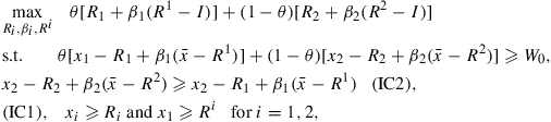
An optimal contract maximizes the principal’s profit subject to giving the agent an expected gross payoff of at least W0. The value of W0 is determined by the amount the agent can contribute to up-front investment, and the relative bargaining powers of the principal and agent. Formally, we would like to solve
where the objective function is the principal’s gross profit (after initial investment in period 1). The constraint (IC2) guarantees that if the agent receives a high cash flow of x2, his payoff if he reveals it truthfully, the left-hand side of (IC2), is at least as good as his payoff if he reports cash flow x1 instead. Note also that we did not write out explicitly the analogous truth-telling constraint (IC1) for the low cash flow realization in period 1. We do not expect it to bind, as verified after we derive the optimal contract.
Theorem 2
An optimal contract is as follows: R1 = R2 = x1, β2 = 1 and
Proof
First, without loss of generality we can take R1 = R2 = x1. Indeed, if Ri < x1 then by increasing Ri to x1 and reducing Ri by βi(x1 − Ri), we get a payoff-equivalent contract in which all constraints are still satisfied.
Second, we claim that β2 = 1. If not, let us increase β2 to 1 and R2 by ![]() . Then the left-hand side of (IC2) does not change, and neither does the agent’s payoff. Furthermore, since (IC2) is satisfied, the new value of R2 is less than or equal to
. Then the left-hand side of (IC2) does not change, and neither does the agent’s payoff. Furthermore, since (IC2) is satisfied, the new value of R2 is less than or equal to
![]()
since β1 ≥ 0, ![]() , and R1 ≤ x1.
, and R1 ≤ x1.
Third, if ![]() , then β1 = 1. Otherwise, we can raise β1 by ɛ and improve total surplus while also improving the agent’s payoff by
, then β1 = 1. Otherwise, we can raise β1 by ɛ and improve total surplus while also improving the agent’s payoff by ![]() (
(![]() is assumed to be sufficiently small so that
is assumed to be sufficiently small so that ![]() . We can transfer this payoff from the agent to the principal by raising R1 by
. We can transfer this payoff from the agent to the principal by raising R1 by ![]() . Since the value of the right-hand side of (IC2) does not change, the contract still satisfies all the constraints, and the principal is strictly better off.
. Since the value of the right-hand side of (IC2) does not change, the contract still satisfies all the constraints, and the principal is strictly better off.
Now, if β1 = β2 = 1, then to satisfy (IC2) the agent cannot be required to pay more than R2 = x1 after high output in period 1, so he gets the payoff of at least ![]() . Thus, this case is relevant only when
. Thus, this case is relevant only when ![]() . If so, the contract provided in part (b) satisfies all constraints and attains first-best; therefore it is optimal.
. If so, the contract provided in part (b) satisfies all constraints and attains first-best; therefore it is optimal.
Fourth, if ![]() then β1 < 1, R1 = x1, and we claim that (IC2) must bind. If not, let us increase β1 by ɛ and at the same time increase R2 by
then β1 < 1, R1 = x1, and we claim that (IC2) must bind. If not, let us increase β1 by ɛ and at the same time increase R2 by ![]() . Then the agent’s expected value remains unchanged and, because total surplus improves, the principal’s value improves. Furthermore, if ɛ is small then (IC2) is still satisfied. We conclude that
. Then the agent’s expected value remains unchanged and, because total surplus improves, the principal’s value improves. Furthermore, if ɛ is small then (IC2) is still satisfied. We conclude that ![]() .
.
Fifth, we can pin down the values of β1 and R2 assuming that the agent gets the expected payoff of exactly ![]() . If so, then using (IC2), the agent’s payoff is
. If so, then using (IC2), the agent’s payoff is
![]()
as in part (a) of the theorem. As W0 moves between ![]() and
and ![]() , β1 spans the entire feasible range of [0, 1].
, β1 spans the entire feasible range of [0, 1].
The principal’s profit
![]()
is a decreasing function of W0, and so it follows immediately that the agent’s expected payoff constraint must bind if ![]() .
.
If ![]() , then setting β1 = 0 satisfies the agent’s reservation payoff constraint, and so the optimal contract is given by part (c) of the theorem.
, then setting β1 = 0 satisfies the agent’s reservation payoff constraint, and so the optimal contract is given by part (c) of the theorem.
Figure 4 illustrates the principal’s profit as a function of W0. Note the special cases of ![]() and
and ![]() . In the former case, the agent obtains financing for the last period if he pays
. In the former case, the agent obtains financing for the last period if he pays ![]() in the first period. Thus, he is indifferent between paying only x1 in period 1 and paying
in the first period. Thus, he is indifferent between paying only x1 in period 1 and paying ![]() in exchange for a round that lets him receive an expected payoff of
in exchange for a round that lets him receive an expected payoff of ![]() and pay x1 in the last period. In the latter case, the agent pays x1 in both rounds, and receives funding for both rounds for sure. Note that on the interval
and pay x1 in the last period. In the latter case, the agent pays x1 in both rounds, and receives funding for both rounds for sure. Note that on the interval ![]() , the slope of the principal’s profit is flatter than −1 because
, the slope of the principal’s profit is flatter than −1 because ![]() . As W0 increases, so does the total surplus because inefficiency due to the agency problem becomes less severe. The inefficiency depends on the probability with which the project does not get funded in the second period. In Section 4, when we discuss the model of DeMarzo and Sannikov (2006), we will see how the slope of the principal’s value function changes in a dynamic setting.
. As W0 increases, so does the total surplus because inefficiency due to the agency problem becomes less severe. The inefficiency depends on the probability with which the project does not get funded in the second period. In Section 4, when we discuss the model of DeMarzo and Sannikov (2006), we will see how the slope of the principal’s value function changes in a dynamic setting.
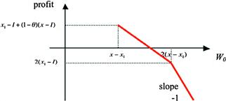
Figure 4 The principal’s profit as a function of the agent’s payoff in the model of Bolton and Sharfstein (1990).
Remark 1
In this model, for all W0 the optimal contract is renegotiation-proof. If the cash flow is low in period 1 so that the contract prescribes project termination (in case R1 = x1 and β1 < 1), the principal and the agent cannot renegotiate to continue the project. Indeed, because the agent just paid out the entire cash flow to the principal, he has no cash left to contribute towards investment in period 2. Thus, the principal always finds it unprofitable to fund new investment.
However, in more complex dynamic models, the optimal contract can easily be not renegotiation-proof, as we will see in Section 4.
Remark 2
If ![]() , then the contract exhibits ex post inefficiency. Bad performance in period 1 may lead to a lack of financing in period 2, even though the profitability of the second period does not depend on performance in period 1.
, then the contract exhibits ex post inefficiency. Bad performance in period 1 may lead to a lack of financing in period 2, even though the profitability of the second period does not depend on performance in period 1.
Remark 3
The optimal contract can be implemented as follows. Initially the firm is funded with 2I − x1. The agent holds equity and the principal holds debt with promised repayments R2 − x1 and x1. In period 1, if the cash flow is high, available cash balance of x2 + I − x1 is sufficient to both make the debt payment and fund investment. If the cash flow is low, then cash balance I is insufficient to both pay debt and fund investment. The principal allows the agent to skip a payment with probability β1, and with probability 1 − β1 triggers default.
2.2 Adverse Selection
If a firm manager has private information about firm fundamentals, it may be difficult to sell informationally sensitive securities, especially equity, to raise funds for investment or share risk. Typically, insiders must retain some of firm’s cash flows in order to signal to the market the quality of the firm. Leland and Pyle (1977) provide a classic model in which firm insiders signal their private information about the quality of fundamentals by retaining shares of equity.
Myers and Majluf (1984) studies the effect of private information on investment decisions. It assumes that financing can be raised only in the form of equity, and that the management acts in the interest of old shareholders. It finds that “if managers have inside information there must be some cases in which that information is so favorable that management, if it acts in the interest of the old stockholders, will refuse to issue shares even if it means passing up a good investment opportunity” (p. 188).
The model is as follows. There is no discounting. At time 0 the management has an investment opportunity that requires investment I. The firm has financial slack S < I (cash + marketable securities) and must raise E = I − S by issuing new equity if it decides to go ahead. If the investment is not made at time 0, the investment opportunity evaporates.
The management knows the value y that the investment opportunity generates and the value x of assets in place. However, from the point of view of the market, these are random variables ![]() . With this information, the market requires the management to sell a fraction α of firm equity in order to raise E.
. With this information, the market requires the management to sell a fraction α of firm equity in order to raise E.
It is assumed that following a decision to issue, the old shareholders remain passive. That is, they “sit tight” if stock is issued; thus the issue goes to a different group of investors.
Definition
An equilibrium consists of a fraction α of equity that has to be issued to raise E, and the investment region M ⊆ [0, ∞) × [0, ∞) such that:
The following simple example illustrates equilibrium.
Example
There are two equally likely states of the world. In state 1, assets in place are worth x = 150, and an investment of I = 100 generates a cash flow of y = 120. In state 2, assets in place are worth x = 50, and an investment of I = 100 generates a cash flow of y = 110. The firm has no financial slack, i.e. S = 0.
In this example there is no equilibrium in which both types of firms invest. An investment by both types would require α = 100/215, since E[x + y] = 215 and E = 100. But then (1 − α) (150 + 120) = (115/215)270 = 144.42 < 150.
There is an equilibrium in which the firm invests only in state 2, by selling the fraction of equity α = 100/160. Since the investment has positive NPV, (1 − α) 160= 60 > 50. In this equilibrium, in state 1 the firm forgoes a positive-NPV project due to the asymmetric information problem.
In general, the investment region ![]() as illustrated in Figure 5.
as illustrated in Figure 5.
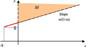
Figure 5 The set of parameters (x, y) for which the firm sells equity.
Assuming that the joint distribution of (x, y) over [0, ∞) × [0, ∞) is characterized by a strictly positive density, the equation
![]()
must have at least one solution. Indeed, note that the left-hand side is continuous in α, and it goes from 0 at α = 0 to infinity as α → 1 and the slope of the lower boundary of M gets steeper.
Theorem 3
In equilibrium firms with low asset value x may issue equity to finance a project with negative NPV, and firms with a high asset value may forgo a project with positive NPV.
Proof
First, we argue that in equilibrium α < E/I. Otherwise, if α ≥ E/I then x + y ≥ I in region M as illustrated in the left panel of Figure 6.

Figure 6 The Proof of Theorem 3.
If so, then
![]()
violating the equilibrium definition.
Since α < E/I, the low corner of M is at a point (0, y) with y < I, as illustrated in the right panel. Therefore, region M includes negative-NPV projects for firms with low asset value x. Also, since α > 0, some positive-NPV projects are not taken by firms with high x.
Of course, it is difficult to issue equity in the presence of informational asymmetries, because equity is very sensitive to private information. In the model of Myers and Majluf (1984), it is assumed that the firm cannot raise funds through other securities, such as debt or hybrid securities. We next discuss a model that investigates optimal security design under asymmetric information, using general securities.
DeMarzo and Duffie (1999) consider a setting in which an issuer owns assets with random cash flows, and wants to raise capital by issuing asset-backed securities. The issuer receives superior private information about the assets’ cash flows after security design stage but before sale. We saw in the overview of Myers and Majluf (1984) that it is difficult to sell equity in the presence of private information, because equity is quite information-sensitive. Here we will allow for general securities, and solve for optimal security design. The desire to issue is motivated by the assumption that the issuer is less patient than the market, e.g. because the issuer has superior investment opportunities. This is captured by assuming that the issuer discounts cash flows at the rate of δ < 1, while the market does not discount.
The model has one period, and the issuer’s assets generate a random cash flow of ![]() at the end of the period. A security is characterized by a non-decreasing function g : [0, ∞) →[0, ∞), which gives the payout to investors at the end of the period as a function of realized cash flow, x. Function g has to satisfy the feasibility constraint g(x) ≤ x. Formally the timeline is as follows:
at the end of the period. A security is characterized by a non-decreasing function g : [0, ∞) →[0, ∞), which gives the payout to investors at the end of the period as a function of realized cash flow, x. Function g has to satisfy the feasibility constraint g(x) ≤ x. Formally the timeline is as follows:
• the issuer designs a security g;
• the issuer learns private information z;
• the issuer chooses the quantity q ∈ [0, 1] of the security to sell;
• the market prices the securities sold at Pg(q) depending, on the quantity sold;
• cash flows are realized, investors are paid according to g, and the issuer receives the remaining cash flow.
The issuer’s expected payoff is given by
![]()
Note that the issuer does not discount the proceeds from the sale of the security, but discounts at rate δ the cash flows received upon the maturity of the assets.
The issuer would like to design a security to maximize her ex ante expected payoff. Formally, given a security g, the perfect Bayesian equilibrium consists of a map z → q such that (1) the issuer chooses q to maximize her expected payoff, (2) given q, the market forms its belief about the issuer’s type according to Bayes rule, and (3) given the belief, the market prices the security at its expected payoff.
The issuer’s optimization problem with respect to q in equilibrium is
![]()
where f = E[g(x)|z] is the expected payoff of the security. Since the issuer’s expected payoff depends on her type z only through f after the security g has been designed, it is convenient to think of f as the issuer’s type in the signaling equilibrium, in which the quantity q is chosen.
Assuming that in equilibrium, quantity sold q( f ) is a continuous function of the value of the security f, the schedule q( f ) can be characterized from the first-order condition
![]()
Using the fact that in equilibrium Pg(q) = f is the inverse of q( f ), so that ![]() , we have:
, we have:
![]()
The constant of integration is pinned down by the condition that the worst type f0 sells q = 1, and so:

From this expression, we see the trade-offs involved in optimal security design. Equity g(x) = x maximizes f0 since it sells all cash flows of the worst type to investors. However, equity is also very informationally sensitive. Therefore, as asset fundamentals z improve, f = E[g(x)|z] rises very fast, leading to very low payoffs for issuers with good fundamentals. It may be possible to raise the expected payoff of issuers with good fundamentals by designing a less informationally sensitive security, that is, making g(x) less sensitive to the cash flow x. However, that has a cost, as the value of f0 ends up lower. It follows that, in comparison with equity, less informationally sensitive securities give lower payoffs to issuers with low-quality assets, but may give significantly higher payoffs to issuers with high-quality assets. Below, we characterize conditions when equity is the optimal security, and when risky debt is.
Intuitively, it is optimal to sell equity if the seller’s private information is small.
Theorem 4
If![]() then g(x) = x is optimal.
then g(x) = x is optimal.
Proof
See Proposition 6 in DeMarzo and Duffie (1999).
If the seller’s private information is not that small, then debt turns out to be optimal under an additional condition.
Definition
Type z0 is called a uniform worst case if ![]() is increasing in x.
is increasing in x.
Theorem 5
If there is a uniform worst case then standard debt is optimal (among securities, for which g(x) is non-decreasing).
Proof
Consider an arbitrary security, characterized by a non-decreasing payoff function g(x). Let us compare it with debt D(x), whose face value is chosen so that
![]()
Then, let us show that for all z ≠ z0,
![]()
Then it follows immediately that the payoff for each type under standard debt is

its payoff under security g.
Since g(x) ≤ x is a security with a non-decreasing payoff, there exists a point x* such that g(x) ≤ D(x) for x ≤ x* and g(x) ≥ D(x) for x > x*, as illustrated in Figure 7.

Figure 7 The Proof of Theorem 5.
We have
![]()
since for all x, ![]() .
.
Intuitively, debt is optimal because if the issuer’s private info changes from z0 to z, then standard debt, in the class of monotone securities, is one that minimizes the increase in the issuer’s private valuation, and thus illiquidity costs.
3 Simple Securities in Dynamic Models
In this section, we explore simple securities in a fully dynamic model, before we consider optimal dynamic security design in the next section. In particular, we focus on the model of Leland (1994), which builds upon the dynamic models of Merton, 1974 and Black and Cox (1976) to explore the trade-offs between the tax advantages of debt and bankruptcy costs.
Merton (1974), Black and Cox (1976), and Leland (1994) investigate the model of a firm that pays no dividends and whose asset value, under the risk-neutral probability measure, follows the geometric Brownian motion:
![]() (1)
(1)
In Eqn (1), Zt is a standard Brownian motion under the risk-neutral measure and r is the risk-free rate. Below, we first describe the classic risky debt valuation model of Merton (1974), in which debt has fixed maturity, and then describe Leland (1994), which focuses on perpetual debt.
Importantly, using both of these models, we are also able to discuss the incentive properties of a particular capital structure. This discussion, which focuses on the sensitivities of the value of equity to the value and volatility of assets, serves as a precursor to the next section that considers optimal security design.
Merton (1974) considers a capital structure that consists of zero-coupon debt with promised payment D and fixed maturity T. The firm defaults at time T if VT < D. If the firm does not default, then equity holders pay off debt (e.g. by borrowing again). As a result, the payoff of equity holders is
![]()
Effectively, equity is a call option on firm assets with maturity T and strike D, and so its value is given by the Black–Scholes formula:
![]()
where ![]() , and N is normal CDF.
, and N is normal CDF.
This simple capital structure highlights incentive problems that typically arise when a firm raises outside financing. The Delta of an option measures the sensitivity of option value to the price of the underlying Vt. The Delta of equity with respect to assets, N(d1), is less than 1. This can lead to debt overhang. Equity holders will not take projects that cost them more than Delta per 1 added to firm value.
Option Vega measures the sensitivity of option value to volatility. Since the Vega > 0 for call options, there is asset substitution. Given the fixed-debt contract in place, equity holders would like to increase the risk of assets, and gradually will if they can.
Leland (1994) explores trade-offs between the tax advantages of debt and bankruptcy costs in a model with perpetual debt, in which the firm’s assets also follow (1). Debt with a continuous coupon rate of C is set at time 0. Due to tax effects, the effective cost of these coupon payments to equity holders is ![]() , where
, where ![]() is the tax rate and
is the tax rate and ![]() is the interest tax shield.3
is the interest tax shield.3
In the version of the model with an endogenous bankruptcy choice, equity holders decide at each moment of time whether to keep paying coupons or default and forfeit the assets to debt holders. Effectively equity holders have a perpetual American put option to sell the firm’s assets for ![]() . It is exercised only when the value of assets drops to the critical boundary VB, which we derive below.
. It is exercised only when the value of assets drops to the critical boundary VB, which we derive below.
The stationary nature of this setting implies that the prices of all securities are functions of V. Since the required rate of return under the risk-neutral measure is r, the value of any security F(V) must satisfy the equation
![]() (2)
(2)
where CF is the cash flow that the security pays and ![]() is the drift of F(V). The appropriate value of CF is C for debt, −(1 − τ)C for equity, and τC for the firm as a whole. Using (1) and Ito’s lemma,
is the drift of F(V). The appropriate value of CF is C for debt, −(1 − τ)C for equity, and τC for the firm as a whole. Using (1) and Ito’s lemma, ![]() , and so the security-pricing Eqn (2) becomes
, and so the security-pricing Eqn (2) becomes
![]()
For any value of CF, this equation has a general solution of the form
![]()
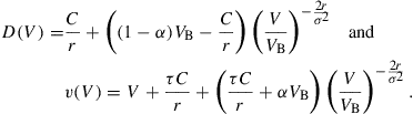
Matching the boundary conditions at the bankruptcy boundary VB and infinity, equity has value
![]()
To find the value of the firm’s debt D(V), as well as the value of the whole firm v(V) = E(V) + D(V), assume that in bankruptcy a fraction α of firm assets VB is lost due to bankruptcy costs. Then
The boundary VB, at which equity holders exercise their option to abandon the assets in the endogenous bankruptcy case, can be determined by the smooth-pasting condition
![]()
This leads to
![]() (3)
(3)
Given C and τ, the point at which equity holders default is independent of the initial value of the assets V0 or bankruptcy costs α. VB is proportional to the debt burden (1 − τ)C, and VB decreases as asset volatility goes up.
Equity holders choose the boundary VB to maximize their payoff, without taking into account the payoff of debt holders. This leads to a conflict of interest. When determining the optimal capital structure in endogenous bankruptcy case ex ante, market participants recognize that ex post equity holders default at the boundary given by (3). Maximizing the value of the firm
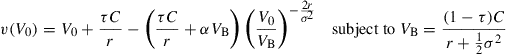
with respect to C, we find that
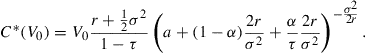
Naturally, the optimal coupon rate is proportional to V0.
As in the Merton model, equity Delta with respect to assets in this model is less than 1. Delta decreases to 0 as V drops towards VB. This phenomenon can cause severe agency problems to arise when equity holders are under water in a richer model where equity holders can take costly actions that may improve the value of the firm. For example, if equity holders were also controlling investment, they would refuse positive-NPV projects when V gets close to VB.
Under alternative conditions determining bankruptcy, such as in the presence of protective debt covenants, agency problems can be less severe near bankruptcy. Equity Delta with respect to asset value could be large near bankruptcy if bankruptcy is forced by the contract, rather than determined by the equity holders’ decision to walk away from the assets. The optimal design of the security held by the “agent”—the firm’s insiders—is the subject of the next section. Section 4 presents several explicit models that capture how the agent’s actions can affect the firm’s value in a dynamic setting.
4 Optimal Dynamic Security Design under Moral Hazard
The foundation of optimal security design under dynamic moral hazard lies in dynamic agency theories, which have been studied by Radner (1985), Rogerson (1985), Green (1987), Spear and Srivastava (1987), Abreu, Pearce, and Stacchetti (1990), and Phelan and Townsend (1991). In corporate finance, discrete-time models of dynamic financing under moral hazard include the work of Albuquerque and Hopenhayn (2004), Clementi and Hopenhayn (2006) and DeMarzo and Fishman (2007a, 2007b). Continuous-time principal-agent models (see Sannikov, 2008), offer particularly tractable methods that have been adopted in corporate finance. Biais et al. (2007) is an important paper that illustrates the relationship between continuous-time and discrete-time methods.
We begin this section by reviewing the work of DeMarzo and Sannikov (2006), which characterizes optimal security design under dynamic moral hazard using continuous-time methods, and that of DeMarzo et al. (2011), which investigates the relationship between agency problems and investment dynamics. After that, we briefly review a number of other models that adopt the dynamic agency framework to study a broader set of issues.
DeMarzo and Sannikov (2006) (hereafter DS) model the same type of moral hazard as the two-period model of Bolton and Scharfstein (1990) which we have already reviewed, in infinite horizon.
The agent has a profitable investment opportunity that, if funded with an initial investment of I > 0, would generate a cash flow stream of the form
![]()
where Zt is a standard Brownian motion. The agent would like to write a contract with the principal (an investor) to fund this project and use it as a collateral to fund the agent’s consumption. The agent would like to borrow money against this project because he has a higher discount rate γ than the market rate r, and also because he may not have sufficient funds to finance the up-front investment.
However, an agency problem exists because the agent privately observes the true cash flows Yt. Thus, the agent may divert some of the cash flows for personal consumption or as perks. The principal only learns about cash flows that are left ![]() after the agent’s diversion action, possibly through the agent’s report. Assume that the cumulative amount of cash diverted
after the agent’s diversion action, possibly through the agent’s report. Assume that the cumulative amount of cash diverted
![]()
must be a continuous non-decreasing process (i.e. the agent cannot send the principal a higher cash flow than realized). It is inefficient to divert cash, so that the agent is able to enjoy only a fraction λ ∈ (0, 1] of diverted cash. In order to solve the agency problem, the contract between the principal and the agent may force a termination of the project in the event that the observed cash flows ![]() are insufficient. In the event of termination, the principal receives the project’s assets, which he values at L, and the agent pursues his outside option with value R. Termination is inefficient, i.e.
are insufficient. In the event of termination, the principal receives the project’s assets, which he values at L, and the agent pursues his outside option with value R. Termination is inefficient, i.e.
![]()
DS derive the optimal contract between the agent and the principal in this setting, which maximizes the principal’s profit subject to a set of constraints, including the incentive constraints. There are no restrictions regarding the form of contracts allowed. That is, contracts can specify in the most general way how the termination time τ and the agent’s compensation dCt depend on the history of observed cash flows ![]() .
.
Because the marginal benefit to the agent from diverting cash is a constant λ, and because the agent can divert cash at an unbounded rate, the optimal contract should not allow any cash flow diversion. Intuitively, it is cheaper to allow the agent to consume some of the project’s cash flows directly, rather than through cash flow diversion behind the principal’s back.
Formally, the optimal contract solves the following constrained optimization problem:
![]() (4)
(4)
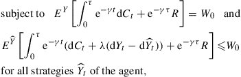
where superscripts Y and ![]() over the expectation highlight that the agent’s compensation dCt, as well as the termination time τ, depend on the agent’s reports. Parameter W0 in the first constraint is the agent’s expected payoff, which is determined by the relative bargaining powers of the principal and agent. Problem (4) is feasible whenever W0 ≥ R.
over the expectation highlight that the agent’s compensation dCt, as well as the termination time τ, depend on the agent’s reports. Parameter W0 in the first constraint is the agent’s expected payoff, which is determined by the relative bargaining powers of the principal and agent. Problem (4) is feasible whenever W0 ≥ R.
The second set of constraints restricts contracts to those in which the agent prefers to abstain from cash flow diversion. This set of contracts can be characterized via a simple condition on the sensitivity of the agent’s continuation payoff to observed cash flows ![]() . For a given contract {τ, C}, the agent’s continuation payoff when he refrains from cash flow diversion is given by
. For a given contract {τ, C}, the agent’s continuation payoff when he refrains from cash flow diversion is given by
![]()
Theorem 6
For any contract {τ, C} there exists a process βt such that
![]() (5)
(5)
and it is optimal for the agent to refrain from cash flow diversion if and only if βt ≥ λ for all t ≤ τ. Also conversely, if a process Wt ≤ R follows(5)until time τ, at which Wτ = R, and satisfies the transversality condition E[1t≤τ e−γt Wt] → 0 as t → ∞, then Wt is the agent’s continuation payoff.
Proof
See DS.
The representation (5) can be derived using the Martingale Representation Theorem, by focusing on the martingale:
![]()
The terms ![]() in the law of motion of Wt are due to simple accounting for the agent’s discount rate, and payoff received by the agent through consumption.
in the law of motion of Wt are due to simple accounting for the agent’s discount rate, and payoff received by the agent through consumption.
The incentive condition is βt ≥ λ because the agent refrains from cash flow diversion if he receives at least λ in the present value of his future payoff for each dollar of cash flow reported to the principal.
Due to Theorem 6, the principal’s problem (4) can be reduced to a stochastic control problem.
Corollary
There is a one-to-one correspondence between contracts {τ, C} that satisfy the constraints of problem(4)and controlled processes
![]()
that satisfy the transversality condition under controls (Ct, βt ≥λ), with τ defined as the first time when Wt hits R.
The control problem is to maximize the principal’s objective (4) by a choice of controls (Ct, βt ≥ λ) that drive the state Wt according to (5), subject to the constraint that time τ occurs when Wt hits R for the first time as well as the transversality condition. To solve the control problem, we can follow an intuitive line of reasoning to conjecture a solution, and then verify that the solution is optimal.
Intuitively, contracting in this setting involves inefficiencies because the agent needs incentives to report cash flows truthfully. The principal provides these incentives by tying the agent’s continuation payoff to performance through the sensitivity coefficient βt ≥ λ. This introduces volatility in the agent’s payoff. A bad history of cash flows drives Wt down to R, and necessitates inefficient termination. Due to this intuition, the choice βt = λ, which minimizes the volatility of Wt while still satisfying the incentive constraints, is optimal.
The choice of the agent’s compensation also involves an interesting trade-off. Because the agent’s discount rate γ is higher than r, it is expensive for the principal to postpone payments to the agent. However, according to (5), early payments to the agent reduce the agent’s continuation payoff Wt and increase the chance that Wt hits R due to a cash flow drawdown. This concern is particularly pressing when Wt is low, so that the chance of termination is significant. Therefore, we conjecture that there is a critical level of ![]() such that it is optimal to pay nothing to the agent when
such that it is optimal to pay nothing to the agent when ![]() , and pay immediately any accumulated continuation payoff in excess of
, and pay immediately any accumulated continuation payoff in excess of ![]() .
.
To summarize, we conjecture a contract of the following form:
In the optimal contract, the agent’s continuation payoff evolves according to
![]()
on the interval ![]() . The agent is paid only when
. The agent is paid only when ![]() , i.e. dCt = 0 if
, i.e. dCt = 0 if ![]() , and otherwise payments dCt are chosen so that Wt is a reflecting process that never exceeds
, and otherwise payments dCt are chosen so that Wt is a reflecting process that never exceeds ![]() . If
. If ![]() , then at time 0 the agent receives a lump-sum payment of
, then at time 0 the agent receives a lump-sum payment of ![]() . Termination occurs when Wt hits the boundary R for the first time.
. Termination occurs when Wt hits the boundary R for the first time.
We still need to determine the optimal level of ![]() . We can do that by valuing the security that the principal is holding under this contract, and then finding
. We can do that by valuing the security that the principal is holding under this contract, and then finding ![]() that maximizes the value of that security. The value of this security is a function of current Wt. As in Leland (1994), we can value the principal’s security through equation
that maximizes the value of that security. The value of this security is a function of current Wt. As in Leland (1994), we can value the principal’s security through equation
![]()
where CF is the cash flow that the security pays and ![]() is the drift of F(W). On
is the drift of F(W). On ![]() , dCt = 0 and so the principal’s expected cash flow is μ. Thus, using Ito’s lemma, F(W) must satisfy
, dCt = 0 and so the principal’s expected cash flow is μ. Thus, using Ito’s lemma, F(W) must satisfy
 (6)
(6)
for all ![]() . This second-order ordinary differentialequation requires two boundary conditions to solve. First, F(R) = L, because the value of the assets to the principal is L when termination occurs. Second,
. This second-order ordinary differentialequation requires two boundary conditions to solve. First, F(R) = L, because the value of the assets to the principal is L when termination occurs. Second, ![]() , because at the point where the agent gets paid it costs the principal one dollar to give the agent an extra dollar of utility. For any choice of
, because at the point where the agent gets paid it costs the principal one dollar to give the agent an extra dollar of utility. For any choice of ![]() , the corresponding solution gives the principal’s value of the contract, in which payments to the agent are made at point
, the corresponding solution gives the principal’s value of the contract, in which payments to the agent are made at point ![]() .
.
So, what is the optimal choice of ![]() ? To answer this question, in Figure 8 we illustrate the phase diagram of solutions to Eqn (6) starting with boundary condition F(R) = L, for different levels of F’(R). For any W ≥ R, it can be shown that F’(W) is increasing in F’(R).4
? To answer this question, in Figure 8 we illustrate the phase diagram of solutions to Eqn (6) starting with boundary condition F(R) = L, for different levels of F’(R). For any W ≥ R, it can be shown that F’(W) is increasing in F’(R).4
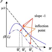
Figure 8 Functions F(W), such that F(R) = L, which solve Eqn (6) with different boundary conditions F’(R).
In this diagram, ![]() maximizes the principal’s profit. This choice corresponds to the top solution, which has a single inflection point
maximizes the principal’s profit. This choice corresponds to the top solution, which has a single inflection point ![]() where
where ![]() . That solution is concave on the interval
. That solution is concave on the interval ![]() , and then it becomes convex. For any other value of
, and then it becomes convex. For any other value of ![]() , the principal’s security has lower value. The bottom solution corresponds to two different choices of
, the principal’s security has lower value. The bottom solution corresponds to two different choices of ![]() , and
, and ![]() . The slope at the inflection point, which is between
. The slope at the inflection point, which is between ![]() and
and ![]() , is steeper than −1. The bottom solution does not correspond to the optimal contract because, by continuity of solutions to differential equations in initial conditions, a solution with a slightly higher slope F’(R) still reaches slope −1 at some point
, is steeper than −1. The bottom solution does not correspond to the optimal contract because, by continuity of solutions to differential equations in initial conditions, a solution with a slightly higher slope F’(R) still reaches slope −1 at some point ![]() , and it is therefore superior (i.e. it is higher than the bottom solution at every point W, and it represents the principal’s value function under the contract, in which the agent is paid at point
, and it is therefore superior (i.e. it is higher than the bottom solution at every point W, and it represents the principal’s value function under the contract, in which the agent is paid at point ![]() ).5
).5
Note also that since ![]() and solution F has an inflection point at
and solution F has an inflection point at ![]() , i.e.
, i.e. ![]() , Eqn (6) implies that
, Eqn (6) implies that
![]()
This equation, which corresponds to the dashed line in Figure 8, can be taken as a condition that determines the optimal level of ![]() . It can be interpreted as follows: it makes sense to postpone payments to the agent to reduce the likelihood of termination, but only up to the point where the expected cash flows exhaust the required returns of the principal and the agent.
. It can be interpreted as follows: it makes sense to postpone payments to the agent to reduce the likelihood of termination, but only up to the point where the expected cash flows exhaust the required returns of the principal and the agent.
We can verify that this contract, which we guessed using intuitive reasoning, is indeed optimal using an argument that we sketch below:
A sketch of the verification argument. Let function F, together with the point ![]() , be determined on
, be determined on ![]() by Eqn (6) and boundary conditions F(R) = L,
by Eqn (6) and boundary conditions F(R) = L, ![]() and
and ![]() . Let us extend F beyond
. Let us extend F beyond ![]() linearly with slope −1. We will show that there is no contract with value higher than F(W0) to the principal.
linearly with slope −1. We will show that there is no contract with value higher than F(W0) to the principal.
For an arbitrary contract {C, τ}, in which the agent’s continuation value follows:
![]()
consider the process ![]() .
.
We claim that Gt is a super-martingale. Differentiating Gt with respect to t, we get
Using the fact that F"(Wt) ≤ 0, and F’(Wt) ≥ −1, we see that Gt is a super-martingale by focusing on its drift.
Therefore, the principal’s profit from this contract is:
![]()
We finish discussing DS by outlining one particular capital structure that implements the optimal contract, and mentioning a few comparative statics results.
The optimal contract can be implemented in many ways, but one particularly attractive implementation involves a credit line. To construct the implementation, we map Wt into the outstanding balance Mt on a credit line, so that point ![]() corresponds to balance Mt = 0, and point R corresponds to the credit limit
corresponds to balance Mt = 0, and point R corresponds to the credit limit ![]() . Then
. Then ![]() evolves according to
evolves according to
![]()
This leads to a capital structure consisting of a credit line, perpetual debt and equity. The agent holds a fraction λ of equity. The principal holds perpetual debt, which receives a flow of payments of ![]() , and the credit line, which receives the project cash flows net of the perpetual debt payments and dividends, and the fraction 1 − λ of equity.6 Total dividends on equity are
, and the credit line, which receives the project cash flows net of the perpetual debt payments and dividends, and the fraction 1 − λ of equity.6 Total dividends on equity are ![]() , and they are paid only when Mt = 0, i.e. the credit line is fully paid off. The interest rate on the credit line equals to the agent’s discount rate γ. The contract triggers termination when the credit line is drawn to the limit.
, and they are paid only when Mt = 0, i.e. the credit line is fully paid off. The interest rate on the credit line equals to the agent’s discount rate γ. The contract triggers termination when the credit line is drawn to the limit.
Note that the cash flows on the securities held by the principal (perpetual debt, credit line, and equity) are the same as in the optimal contract based on Wt. Indeed, when ![]() then the principal receives just the reported cash flows
then the principal receives just the reported cash flows ![]() . Perpetual debt pays a flow of
. Perpetual debt pays a flow of ![]() , and the credit line receives the payments of
, and the credit line receives the payments of ![]() net of the coupon payments on perpetual debt
net of the coupon payments on perpetual debt ![]() . The interest rate charged on the credit line increases its balance, but does not generate an actual cash flow. At point
. The interest rate charged on the credit line increases its balance, but does not generate an actual cash flow. At point ![]() , the agent receives dCt in each contract, and the principal receives the rest,
, the agent receives dCt in each contract, and the principal receives the rest, ![]() .
.
DS verify that under this implementation, the agent has incentives to refrain from cash flow diversion, and instead chooses to use firm cash flows to pay down the credit line, and pay dividends only when the credit line is fully paid off.
The continuous-time formulation makes analytic comparative statics possible in this dynamic contracting setting. For example, the optimal mix of credit line and debt depends on the volatility of cash flows σ and the agent’s discount rate γ.The implementation uses a longer credit line when σ is larger or γ is smaller. See DS for details, and other comparative statics results.
Besides creating a convenient methodology that is applicable to study a range of issues, the model of DS has a number of important economic implications. The optimal contract clearly divides the risks between the agent, the firm insider, and outside investors. The model does not have specific predictions regarding the division of cash flows among outside investors: the Modigliani–Miller theorem holds with respect to those cash flows. The implementation of the optimal contract in the form of a credit line suggests one way to divide these cash flows between outside equity holders and debt holders. Certainly, the implementation is not unique, e.g. Biais et al. (2007) provide an alternative implementation that maps the agent’s continuation payoff Wt into the firm’s cash balance. In any case, it is convenient to link Wt to some measure of the firm’s financial slack.
In this interpretation, the model has a number of important predictions. Past performance is positively related to the firm’s payouts, and the firm’s financial slack. Following poor performance, firms stop paying dividends and may be liquidated inefficiently, even when past performance is uncorrelated with future profitability. The firm’s manager should be exposed to the risk of the firm—he should be compensated with a non-tradable stake of the firm’s equity.
Remark
DS also present a variation of the model, in which the agency problem involves costly effort input rather than cash flow diversion. Specifically, they assume that the principal observes cash flows
![]()
The agent gets a private benefit of B = λA if he shirks.
They show that the optimal contract is the same as in the baseline model (with cash flow diversion), and it gives the agent incentives to work until the termination time τ, if and only if the following condition is satisfied:
![]() (7)
(7)
Zhu (2011) solves for the optimal contract with shirking in this variation of the DS model, when condition (7) is violated. We summarize the findings of Zhu (2011) in Section 4.1.
DeMarzo et al. (2011) (hereafter DFHW) investigate how dynamic agency problems affect the scale of the firm. They use the agency model of DS, and add investment decisions that are observable and contractible.
The firm’s capital stock evolves according to
![]()
where ιt is the cost of investment per unit of capital, and function Φ satisfies Φ(0) = 0, Φ’ > 0 and Φ” ≤ 0. In the absence of investment, capital simply depreciates at rate δ. The concavity of function Φ reflects adjustment costs.7
After accounting for investment and adjustment costs, the firm’s cumulative cash flow process takes the form
![]()
The agent’s action at ≤ 1 reduces the mean of cash flows. Setting at < 1 is inefficient, but it gives the agent a private benefit flow of λ(1 − at)Kt. In the event of termination, which may be required to solve the agency problem, the agent receives the payoff of R = 0, and the principal receives value ![]() from the project’s assets, where
from the project’s assets, where ![]() because the firm can always liquidate by disinvesting. The agent’s discount rate γ is higher than the principal’s discount rate r.
because the firm can always liquidate by disinvesting. The agent’s discount rate γ is higher than the principal’s discount rate r.
The range of possible contracts specify how the cash flows that the agent is allowed to keep Ct, the termination time τ, and the rate of investment ιt depend on the entire history of firm performance {Ys, s ∈ [0, t]}. For the same reasons as in DS, we know that the optimal contract has to create incentives for the agent to always choose at = 1. Formally, the optimal contracting problem is:

In this setting, for an arbitrary contract (τ, C, ι), the law of motion of the agent’s continuation payoff when he follows the strategy {at = 1} is
![]()
The incentive constraint is βt ≥ λ.
The principal’s value function F(Wt, Kt) under the optimal policy depends on both Wt and Kt. It must satisfy the Bellman equation
![]()
Due to the scale-invariance properties of the model, DFHW conjecture that the value function has the form F(W, K) = f(w)K, where w = W/K. Then wt = Wt/Kt follows:
![]()
and the Bellman equation reduces to
![]()
The solution to this equation can be found using similar logic as we used in the discussion of DS.
Theorem 7
The principal’s value function is of the form F(W, K) = Kf(W/K). Function f is concave, and satisfies the equation
![]() (8)
(8)
on the interval![]() determined by the boundary conditions
determined by the boundary conditions
![]()
In the optimal contract, the agent’s compensation, investment and termination time τ are determined by two state variables: Kt and Wt. The law of motion of Wt is determined contractually by
![]()
where payments dCt are set to 0 for![]() and chosen to reflect Wt at the boundary
and chosen to reflect Wt at the boundary![]()
![]()
. The investment rate ιt maximizesand τ is the time when Wt hits 0 for the first time.
Proof
See DFHW.
How does the investment rate under the optimal contract depend on w, and how does it compare to the first-best investment rate? Because f is a concave function, ![]() is increasing in w, and so ι increases with w (see Figure 9 for a geometric interpretation).
is increasing in w, and so ι increases with w (see Figure 9 for a geometric interpretation).

Figure 9 Since f(w) is a concave function, f(w) − wf’(w) increases in w.
Moreover, the first-best investment rate and the corresponding value of capital can be found from
![]()
At the same time, from Eqn (8) and the boundary conditions at ![]() ,
,
It follows that at ![]() , the optimal rate of investment is less than first-best, and the value of the firm per unit of capital (measured as the sum of the principal’s and agent’s payoffs) is also less than qFB.
, the optimal rate of investment is less than first-best, and the value of the firm per unit of capital (measured as the sum of the principal’s and agent’s payoffs) is also less than qFB.
Both the average Tobin’s q of the firm’s assets
![]()
and the marginal q
![]()
are increasing in w. Moreover, because f’(w) ≥ −1, it follows that
![]()
Empirically, the average q (which is easy to measure) is often used empirically as a proxy for the marginal q, following the results of Hayashi (1982). However, even though the model of DFHW exhibits the same homogeneity properties as Hayashi (1982), here the marginal and average q are not the same, due to agency costs. The difference between average and marginal q’s depend on w, and thus the history of firm performance.
The model has the following predictions about the relationship between investment, Tobin’s q, and the firm’s financial slack w:
• Financial slack is positively related to past performance.
• Average and marginal q, as well as investment, are increasing with financial slack.
• The agent’s cash compensation increases with financial slack.
• The maximal level of financial slack is higher for firms with more volatile cash flows and lower liquidation values.
In general, the model predicts that investment is positively correlated with profits, past investment, financial slack, and managerial compensation, even with time-invariant investment opportunities.
DS as well as DFHW serve as a microfoundation of financing frictions that exist in the presence of agency problems. Many papers assume a set of financial frictions, instead of deriving them, and instead devote attention to the implications of these frictions on the issues of investment and financing policies as well as risk management. For example Rampini and Vishwanathan (2010, 2012) assume financing frictions in the form of collateral constraints in a partial equilibrium setting. Brunnermeier and Sannikov (2011) and He and Krishnamurthy (2012) assume constraints with respect to equity issuance, together with restrictions on hedging of certain aggregate risks, to study the implications of frictions on the issues financial stability in general equilibrium settings.
The models of Bolton, Chen, and Wang (2011, 2012) (hereafter BCW) are particularly close to DFHW in how they model the firm’s production technology, but they assume financial frictions directly instead of explicitly modeling an agency problem. Specifically, BCW assume that the firm’s production and investment technology is governed by equations
![]()
These equations are identical to those of DFHW, assuming that the managerial compensation contract in place enforces full effort, at = 1. Instead of modeling the agent’s incentives explicitly, BCW assume financial frictions that are related to the features of the optimal contract that motivate effort. Specifically, they assume that the firm maintains a cash balance (recall the implementations of the optimal contract in DS and Biais et al. (2007)) and that it is costly to issue new equity when the firm runs out of cash. In DS, new equity is issued only when the old manager is fired and replaced with a new manager. In addition, BCW assume that it is costly to keep cash inside the firm instead of paying it out to shareholders, just as in DS it is costly to postpone payments to the agent as the agent is less patient than the principal. Under the optimal policy in BCW, the firm’s financial slack is sensitive to the firm’s cash flows, and evolves between endpoints where dividend payouts are made after good performance and new equity is issued under poor performance. Thus, BCW present a simple dynamic model that captures many of the features of the optimal contract of DS and DFHW without delving into the details of an agency problem explicitly.
4.1 Other Models that Involve Dynamic Moral Hazard
A number of papers adapt a continuous-time dynamic agency framework to study the interaction between agency problems and various other issues. We briefly review several of them here. We focus, for the most part, on the technical elements of these models.
Piskorski and Tchistyi (2010), who consider the problem of optimal mortgage design, have a number of important contributions. First, they adapt a model similar to that of DS to the study of mortgages. Second, they investigate what happens in the optimal contract when market conditions exogenously change. They focus specifically on changes of market interest rates and find that it is optimal to tighten the agent’s access to credit when interest rates rise.
The market interest rate in the model of Piskorski and Tchistyi (2010) is a Poisson switching process with two levels {rL, rH}, and the switching intensity from interest rate ri to rj, j ≠ i, given by δ(ri). The cash flow process
![]()
is interpreted as the borrower’s income, which is unobservable. It is assumed that the borrower can hide income without any cost, so parameter λ in DS is set to 1.
In any incentive-compatible contract the agent’s continuation value follows:
![]()
where ![]() is the agent’s continuation value conditional on the event that the interest rate switches at time t, and the incentive constraint is βt ≥ 1.
is the agent’s continuation value conditional on the event that the interest rate switches at time t, and the incentive constraint is βt ≥ 1.
The principal’s value function Fi(Wt) depends on two state variables—the agent’s continuation value Wt and the current interest rate rt = ri. It is characterized by the system of two equations:
for i = L, H and j ≠ i, with the familiar boundary conditions
![]()
Under the optimal contract, the agent’s continuation value jumps from Wt to ![]() whenever the interest rate switches. A key equation that determines the jump in the agent’s continuation value, when the interest rate jumps from rt− = ri to rt = rj at time t, is the first-order condition
whenever the interest rate switches. A key equation that determines the jump in the agent’s continuation value, when the interest rate jumps from rt− = ri to rt = rj at time t, is the first-order condition
![]() (9)
(9)
We would like to emphasize that condition (9) arises very commonly in models where a state switches via a Poisson process.
Piskorski and Tchistyi (2010) offer several implementations of the optimal contract. In particular, the variable Wt can be mapped into the balance on the homeowner’s home equity line of credit. The changes in the value of Wt in response to interest rate shifts can be linked to some properties of adjustable-rate mortgages. In particular, it is a feature of the optimal contract that the agent’s default probability rises when the interest rates increase.
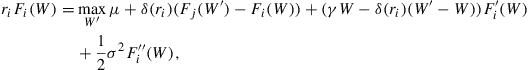
Hoffmann and Pfeil (2010) consider a dynamic agency model, in which firm profitability experiences observable shocks. Their model builds upon DS, except that they allow for Poisson shocks that change the expected rate of cash flows μ. One of the key messages of Hoffmann and Pfeil (2010) is that, despite conventional intuition, the optimal contract rewards the agent for luck when it is correlated with the firm’s future profitability.
Here we review a variation of their model. Assume that the expected rate of cash flows is a Poisson switching process with values {μL, μH}, so that
![]()
The switching intensity from state μi to μj, j ≠ i, is given by δ(μi).8 The agency problem is the same as in DS: the agent can divert cash flows, and he receives benefit equal to a fraction λ ∈ (0, 1] of the diverted cash flows.
The optimal contract depends on μt and the agent’s continuation value Wt, which follows:
![]()
The principal’s value function solves the system of two equations

for i = L, H and j ≠ i, with the familiar boundary conditions
![]()
The most important point of this paper is that under the optimal contract the agent is rewarded for luck, i.e. when the mean of cash flows jumps from μL to μH. This conclusion seems to contradict the conventional wisdom of Holmstrom and Milgrom (1991); that it is optimal to filter out factors outside the manger’s control when evaluating the agent’s performance. An example of this involves the evaluation of fund manager performance relative a benchmark index, rather than in absolute terms. However, in the model of Hoffmann and Pfeil (2010) it is optimal to reward the manager for luck because of the dynamic feature of the model that luck is positively related to future profitability.9
Whenever the mean of cash flows switches from μi to μj, the jump in the agent’s continuation value satisfies the first-order condition
![]()
We have already encountered a similar condition in Piskorski and Tchistyi (2010), in the event that the interest rate jumps.
He (2009) considers a dynamic agency model in which both the agent’s hidden actions and shocks affect the scale of the firm, rather than the current cash flow. Apart from this distinction, the model has many similarities to that of DFHW.
Below we present an extension of the model of He (2009), which incorporates investment decisions that affect the scale of the firm. This model can be a convenient option for applications, as it has different moment properties from DFHW (e.g. firm cash flows are highly correlated in the model of He (2009)—they follow a random walk—but uncorrelated in the model of DFHW).
Consider a firm, whose cash flow is given by
![]()
where ιt is the investment rate and Kt is the firm’s capital, both of which are observable. The firm’s capital follows:
![]()
if the agent works and
![]()
if the agent shirks, where ![]() . Neither the shocks Zt nor the agent’s actions are observable. The agent gets a private benefit of BKt from shirking, where B ≥ 0. Both the agent and the principal are risk-neutral, and the agent’s discount rate is γ ≥ r, where r is the principal’s discount rate.10 In the event of termination, the agent’s outside option is 0, and the value of the assets to the principal is given by
. Neither the shocks Zt nor the agent’s actions are observable. The agent gets a private benefit of BKt from shirking, where B ≥ 0. Both the agent and the principal are risk-neutral, and the agent’s discount rate is γ ≥ r, where r is the principal’s discount rate.10 In the event of termination, the agent’s outside option is 0, and the value of the assets to the principal is given by ![]() , where
, where
![]()
Assume that the difference ![]() and parameter B are such that it is optimal to implement working at all times until termination.
and parameter B are such that it is optimal to implement working at all times until termination.
For a given contract, if the law of motion of the agent’s continuation value is given by
![]()
then the incentive constraint to ensure that it is optimal for the agent to work is βt ≥ λ, where λ = B/(![]() ). The optimal contract sets βt = λ.
). The optimal contract sets βt = λ.
The principal’s value function F(W, K) satisfies the HJB equation
![]()
As in DFHW, the scale-invariance properties of the model imply that the solution must have the form F(W, K) = f(w)K, where w = W/K. By Ito’s lemma, wt = Wt/Kt follows:
![]()
and the HJB equation, in the region where dCt = 0, reduces to
![]()
If γ > r, then the relevant boundary conditions that determine the function f(w) as well as the point ![]() where the agent gets paid are
where the agent gets paid are
![]()
as in DFHW. Point ![]() is a reflecting boundary of the process wt.
is a reflecting boundary of the process wt.
If γ = r, then ![]() and f(w) must satisfy
and f(w) must satisfy
![]()
and the process wt becomes absorbed when it hits ![]() . When that happens, inefficiency completely disappears, and the solution is first-best. In both cases, termination occurs when wt hits 0.
. When that happens, inefficiency completely disappears, and the solution is first-best. In both cases, termination occurs when wt hits 0.
Zhu (2011) provides a general solution to the variation of the DS model with costly effort. Recall that in this model the principal observes cash flows
![]()
The agent gets a private benefit of B = λA if he shirks. This model is similar to the baseline cash flow diversion model of DS, except that the rate, at which the agent can divert cash flows, is bounded by A.
Here we review the results of Zhu (2011), specializing them to the case when the agent’s outside option is R = 0. The form of the optimal contract depends on the region in the space of payoff pairs of the agent and principal, in which the point (λA/γ, (μ − A)/r) lies.
Denote by F(W) the principal’s value function in the baseline model of DS. Recall that this function solves Eqn (6) with boundary conditions ![]() ,
, ![]() and
and ![]() (or, equivalently,
(or, equivalently, ![]() ). Furthermore, let
). Furthermore, let
![]()
Function g(w) bounds region A in Figure 10.

Figure 10 Regions that determine the form of the optimal contract.
The boundary between regions B and D is the locus of points, where solutions ![]() to Eqn (6) with boundary conditions
to Eqn (6) with boundary conditions ![]() and
and ![]() reach slope 0. The boundary between regions C and D is the locus of points, where solutions
reach slope 0. The boundary between regions C and D is the locus of points, where solutions ![]() to Eqn (6) with boundary conditions
to Eqn (6) with boundary conditions ![]() and
and ![]() , for some
, for some ![]() , reach slope 0.
, reach slope 0.
The principal’s value function in the optimal contract can be found as follows:
Case A: If point (λA/γ, (μ − A)/r) falls in region A, then the optimal contract is identical to that in the baseline setting of DS (as demonstrated in Section III of DS).
Case B: If point (λA/γ, (μ − A)/r) falls in region B, then the principal’s value function is determined by solving (6) with boundary conditions ![]() and
and ![]() on an interval
on an interval ![]() and equation
and equation
![]() (10)
(10)
on ![]() , with
, with ![]() . The two portions of
. The two portions of ![]() must merge at
must merge at ![]() in a differentiable manner.The second derivaties must also match (i.e. the supercontact condition has to hold) to ensure that
in a differentiable manner.The second derivaties must also match (i.e. the supercontact condition has to hold) to ensure that ![]() is the largest function that satisfies these conditions.
is the largest function that satisfies these conditions.
Case C: If point (λA/γ, (μ − A)/r) falls in region C, then the principal’s value function is determined by solving (6) with boundary conditions ![]() and
and ![]() on an interval
on an interval ![]() , and Eqn (10) for
, and Eqn (10) for ![]() . The two portions of
. The two portions of ![]() merge at
merge at ![]() in a differentiable manner.
in a differentiable manner.
Case D: If point (λA/γ, (μ − A)/r) falls in region A, then the optimal contract does not give the agent incentives to work in any region.
In both cases B and C, function ![]() is maximized at a point where it satisfies Eqn (6). Thus, if the principal can start the contract at point W0 where his profit is maximized, then the agent will be initially putting effort, and his continuation value will evolve according to:
is maximized at a point where it satisfies Eqn (6). Thus, if the principal can start the contract at point W0 where his profit is maximized, then the agent will be initially putting effort, and his continuation value will evolve according to:
![]()
In case B, the agent is putting in effort while ![]() ; at the left endpoint of this interval the agent is fired, and the right endpoint the agent is allowed to shirk temporarily. Point
; at the left endpoint of this interval the agent is fired, and the right endpoint the agent is allowed to shirk temporarily. Point ![]() is a sticky reflecting boundary of the process Wt. In case C, the agent is putting in effort when
is a sticky reflecting boundary of the process Wt. In case C, the agent is putting in effort when ![]() . At point
. At point ![]() the agent is paid so that Wt reflects at
the agent is paid so that Wt reflects at ![]() . Point
. Point ![]() is a sticky reflecting boundary: at that point the agent shirks and consumes private benefits temporarily (which is not so attractive for the agent because in region C, λA/γ is low).
is a sticky reflecting boundary: at that point the agent shirks and consumes private benefits temporarily (which is not so attractive for the agent because in region C, λA/γ is low).
Biais, Mariotti, Rochet, and Villeneuve (2010) (hereafter BMRV) adapt the agency framework to settings where the agent’s action, e.g. negligence, may lead to large losses. These situations are common in practice, and often the damage is significantly greater than what the agent can cover. BMRV study the question of optimal incentive provision in these settings. They find that losses often require the downsizing of operations.
Formally, BMRV assume that performance-related information takes the form of a Poisson process, rather than a Brownian one. Like DFHW, they also allow for investment (and disinvestment) that changes the scale of the project. They assume a production technology that uses capital Kt to produce a cash flow of
![]()
The term M dNt in the expression for dYt represents possible losses (which translate to cash flow losses of the size KtM). A loss arrives when the counting Poisson process Nt jumps up by 1, and the intensity of losses Ψt depends on the agent’s unobservable action. The agent has two actions: working and shirking. The impact of these actions on the intensity of losses, as well as the agent’s private benefit, are summarized as follows:

The investment function Φ is increasing and concave. BMRV take δ = 0 and consider a particular form of Φ represented in Figure 11.11 That is, it is possible to costlessly destroy arbitrary amounts of capital, and build new capital at cost c, as long as the growth rate does not exceed g < r.

Figure 11 The investment function in the setting of BMRV.
The agent’s and principal’s preferences over consumption streams are identical to those of DS: both the principal and the agent are risk-neutral, the agent’s discount rate is given by γ > r, and the agent can consume only non-negative amounts. Moreover, the agent’s outside option is assumed to be 0 as in DFHW and He (2009).
BMRV mainly focus on parameters, for which it is optimal to give the agent incentives to work at all times, the maximal risk prevention case. We focus on this case here.
The optimal contract is based on two state variables: the agent’s continuation payoff Wt and the size of the firm Kt. Denote the principal’s value function by F(Wt, Kt).
The agent’s continuation value follows:
![]()
The incentive constraint is
![]()
If this constraint holds, then the benefit from shirking is not greater than the negative impact of shirking on the agent’s continuation payoff, i.e. AKt ≤ βtΔψMKt. Naturally, the optimal contract sets βt = λ.
Because information about the agent’s performance arrives via a Poisson process, one has to take into account that it is impossible to give the agent incentives to work when Wt ∈ [0, λMKt). The reason is that a required punishment in the event of a loss would reduce the agent’s continuation payoff by at least λMKt, below the agent’s outside option.12 As a result, if the agent’s continuation payoff ever falls below λMKt, the optimal contract prescribes either randomization that lowers Wt to 0 or boosts it to λMKt, or downsizing that reduces the firm’s capital to Wt/(λM).
Due to the scale-invariance properties of the model,
![]()
When Wt ≤ λMKt, i.e. w ≤ λM, f is a linear function of the form ![]() . The two-dimensional Bellman equation for F(W, K) can be reduced to a one-dimensional equation by a method similar to that used in DFHW. The equation takes the form
. The two-dimensional Bellman equation for F(W, K) can be reduced to a one-dimensional equation by a method similar to that used in DFHW. The equation takes the form

on the interval ![]() , and it must satisfy the boundary conditions
, and it must satisfy the boundary conditions
![]()
Figure 12 illustrates the form of function f in this model.

Figure 12 Function f in the model of BMRV.
The optimal investment rate ι solves
![]()
as in DFHW. Because f is a concave function, it follows that ![]() is increasing in w; thus the rate of investment is increasing in the firm’s financial slack.
is increasing in w; thus the rate of investment is increasing in the firm’s financial slack.
For the specific piecewise linear form of function Φ(ι) assumed in BMRV, the optimal investment rate is
![]()
Effectively, investment happens when wt exceeds a critical level of wi, where
![]()
BMRV has an important implication about how the contract gives incentives to the agent to work to prevent losses. Once wt reaches ![]() , the agent is paid a continuous stream of payments until the next loss. If a loss occurs, payments are suspended and the agent has to wait a fixed amount of time before the payments resume. If another loss occurs, the agent has to wait longer. Too many losses in a row lead to a partial downsizing or liquidation.13
, the agent is paid a continuous stream of payments until the next loss. If a loss occurs, payments are suspended and the agent has to wait a fixed amount of time before the payments resume. If another loss occurs, the agent has to wait longer. Too many losses in a row lead to a partial downsizing or liquidation.13
5 Asymmetric Information in Dynamic Settings
From the static models of Section 3, we know that when asymmetric information is present, it is difficult for firms to raise money for positive-NPV projects. The problem is particularly severe with equity issuance, as its value is highly sensitive to the private information of firm management. In equilibrium, firms raise financing for new investments by selling equity if their assets are overvalued by the market, but may refrain from investing if their assets are undervalued. Upon the announcement of issuance, the market revises its belief about the firm’s assets down, and the firm’s stock price drops. The problem is less severe with debt, which is less informationally sensitive. Firms with good private information are able to raise more money by issuing less informationally sensitive securities.
5.1 Static Contracts in Dynamic Settings
A number of new issues come to light once we think about the time dimension. Below we review several models that highlight these issues, starting with models that incorporate static contracts in dynamic settings.14Lucas and McDonald (1990) consider a model in which firms can raise money for investment opportunities only by issuing equity. Investment opportunities can be postponed, and inside information about assets in place is time varying. In equilibrium, managers of overvalued firms issue equity to finance the investment right away, while managers of undervalued firms wait to issue until their private information becomes public. Stock prices tend to drop upon the announcement of issuance, and generate high abnormal returns prior to issuance.
The model of Lucas and McDonald (1990) motivates us to think about further issues that are likely to arise in dynamic settings with adverse selection. First, while in the model of Lucas and McDonald (1990) managers carry private information for only one period before it becomes public, in more elaborate models managers can signal the quality of their information by waiting. Second, the distribution of private information can change over time: if managers of undervalued firms wait to issue, their proportion in the market can rise over time, alleviating the problem of asymmetric information. This can lead to hot markets when the dilution problem due to asymmetric information is less severe as more high-quality firms sell securities, and cold markets, during which high-quality firms wait and only low-quality firms, or firms with dire capital needs, issue. Third, firms can issue securities other than equity and can build up financial slack during times when the informational problem is less severe.
The model of Daley and Green (2012) sheds light on some of these issues. Specifically, in their setting the seller/issuer, who has persistent private information about asset quality, can signal by waiting. Market belief about the seller’s private information tends to rise during the periods of non-issuance. An improvement of market belief about asset quality leads to a hot market, in which sellers issue regardless of private information. Interestingly, the equilibrium also features a regime where the market freezes, i.e. issuance becomes suspended until further arrival of news.
The models of Lucas and McDonald (1990) and Daley and Green (2012) only give a flavor of many interesting issues that arise in dynamic adverse selection models with simple contracts. A number of other papers look at these issues both empirically and theoretically, including Baker and Wurgler (2002) and Hennessy, Livdan, and Miranda (2008). Market dynamics with adverse selection is also a fruitful area for future research, as a lot of interesting questions have not been answered.
It turns out that many adverse selection frictions become significantly less severe once dynamic contracts are allowed. We finish this section by quickly revisiting Lucas and McDonald (1990) and Daley and Green (2012) with the perspective of dynamic contracts, and review several insights about optimal dynamic contracting under adverse selection.
Lucas and McDonald (1990) consider an infinite-horizon model in which firms have assets in place and may have investment opportunities. For simplicity, the risk-free rate is assumed to be 0. In each period t, the market perceives that the value of the firm’s assets in place is At. At the same time, the manager learns the next period’s value of the firm’s assets, which is
![]()
It is assumed that u > d, so that if At+1 = uAt, the firm is undervalued on the market, and if At+1 = dAt, the firm is overvalued.
In addition, the manager knows whether the firm has an investment opportunity in that period. If an opportunity exists, it requires an investment of KAt, and generates value ![]() in the next period (net of the underwriting fees). It is assumed that a firm can raise money for investment only by issuing equity. As in Myers and Majluf (1984), the manager cares about the firm’s old shareholders.
in the next period (net of the underwriting fees). It is assumed that a firm can raise money for investment only by issuing equity. As in Myers and Majluf (1984), the manager cares about the firm’s old shareholders.
In addition, the following assumptions are made. Between periods t − 1 and t the firm is liquidated for exogenous reasons with probability 1 − ρ, and generates a payoff of At to shareholders. Investment opportunities are random: if the firm has an investment opportunity in period t that it does not take, it still has an investment opportunity in period t + 1. If the firm took its opportunity in period t, or did not have one altogether, it gets an investment opportunity in period t + 1 with probability q.
Lucas and McDonald (1990) focus on an equilibrium, in which firms with an investment opportunity issue equity to finance it only if they are overvalued, and undervalued firms postpone the opportunity. Parameter restrictions are imposed to ensure that overvalued firms without an investment project and undervalued firms do not want to issue (e.g. due to high underwriting costs). Then upon issuance, new investors will infer that At+1 = dAt and that the firm has an investment opportunity. Based on this belief, investors then demand in exchange for capital KAt an appropriate fraction of the firm s, such that they break even.
Due to scale invariance, the manager’s valuation of the firm is of the form V(a, b)At, where a = u or d depending on the value of At+1, and b = 0 or β, depending on whether the firm has an investment opportunity or not. The value function satisfies the following recursive equations in equilibrium:
![]()
for a = u, d
![]()
since K = s(dβ + K + V(d, β)) to ensure that the firm’s new investors break even.
While V(a, b)At is the manager’s valuation of the firm based on his private information, market valuation of the firm will depend on its belief about manager’s information. In particular, in period t, prior to issue announcement, market will believe that a = u with probability p and d with probability 1 − p. In addition, the probability that the firm has a project is increasing in the number of periods n its stock has gone up (and thus the firm had been undervalued in the prior period, and unable to raise funding for the project). The probability that the firm has a project is:
![]()
and so market valuation of the firm’s stock prior to issue announcement is:
![]()
Since V(a, β) > V(a, 0), the value of the firm is increasing in the number of periods its asset value has gone up.
If the firm decides to issue, its market value immediately changes to V(d, β). The decision to issue reveals two pieces of news to the market: bad news that the firm’s asset value will go down in the next period, and good news that the firm has an investment opportunity. If n is large, then P(n) ![]() pV(u, β) + (1 − p)V(d, β) > V(d, β), and the price of the firm drops for sure upon announcement. In this case, the good news that the firm has a project is not really news. If n is small, then stock price reaction to equity issue announcement may be ambiguous.
pV(u, β) + (1 − p)V(d, β) > V(d, β), and the price of the firm drops for sure upon announcement. In this case, the good news that the firm has a project is not really news. If n is small, then stock price reaction to equity issue announcement may be ambiguous.
The model predicts that the firm generates a positive abnormal return prior to issue. This happens because the decision to not issue is related to good private information about the firm’s asset value. The model also predicts that, usually, the firm’s share price should drop upon the announcement of issuance, particularly after long periods of stock price increases.
Daley and Green (2012) consider a dynamic asset market with asymmetric information. They investigate how trade patterns change over time as information is gradually revealed to buyers, who continuously update their beliefs about asset quality. The equilibrium they derive has a very interesting feature of market breakdown: a period when trade stops even though there are beneficial trading opportunities, and sellers have incentives to strategically wait for improved market conditions.
The model has one seller of the asset and a continuum of competitive buyers. The seller has one asset whose quality θ ∈ {L, H} is privately known to the seller. The seller derives a payoff flow of Kθ from the asset until a trade occurs, and any buyer who purchases the asset is able to derive a higher payoff flow of Vθ > Kθ after the time of the trade. Quality H generates more value, i.e. VH > VL and KH > KL. Buyers continuously make offers to the seller until a sale occurs. After the sale, the purchaser holds the asset in perpetuity.15 Denote by Wt/r the highest offer that the buyers make to the seller at time t in equilibrium, where r is the common discount rate of the seller and all buyers.
Buyers initially believe that the seller is type H with probability π0 ∈ (0, 1). They update their belief from the signal Xt that follows
![]()
where μL < μH, as well as from the seller’s decisions. Ignoring the information about the seller’s decisions, Bayes rule implies that the buyers’ belief about the seller’s type would evolve according to16
![]()
The variable zt ∈ (−∞, ∞) is more convenient to work with than the belief πt ∈ (0, 1).
Furthermore, Daley and Green (2012) show that if we take into account the seller’s decisions, then the absence of trade is always good information about the seller’s type. That is, type H would never trade—i.e. he strictly prefers to wait for future offers—whenever type L prefers to wait or is indifferent. Intuitively, this is true because type H gets a higher payoff flow and more favorable news than type L from holding on to the asset. If no trade is good news, then conditional on the absence of trades, the process zt that determines the buyers’ beliefs about the seller’s type follows:
![]() (11)
(11)
where Qt is a non-decreasing process.
It turns out that the equilibrium is characterized by three regimes:
• z ≤ α, where type H does not trade and type L accepts the offer of VL with probability that is less than 1, such that the posterior zt jumps up to α;
• z ∈ (α, β), where neither type trades, and
• z ≥ β, where both types for sure accept the price of Wt = (1 − πt)VL + πtVH.
Therefore, the process Qt is such that α is a reflecting boundary of the system, and dQt = 0 on the interval (α, β).
For expositional reasons, we will assume that the equilibrium takes this form and derive equations that determine the boundaries α and β, as well as the value functions of both types of the seller. On the interval [α, β], the value functions of the two types of sellers satisfy the HJB equation (see Footnote 15):
![]() (12)
(12)
with the “+” sign if θ = H, and the “−” sign if θ = L. The value function FL(z) of type L reaches the level of VL at point z = α and stays at VL on the entire interval (−∞, α). Moreover, both functions FH(z) and FL(z) reach the level of
![]() (13)
(13)
at point z = β, and satisfy Eqn (13) for all z ∈ [β, ∞). In addition, because α is a reflecting boundary of the system, ![]() .
.
Functions FH(z) and FL(z) that solve the second-order ordinary differential equation (12), together with the two boundaries α and β, can be fully determined through six boundary conditions. In addition to the five conditions that we have already identified, ![]() and FH(β) = FL(β) = Ψ(β), Daley and Green (2012) add a sixth condition of
and FH(β) = FL(β) = Ψ(β), Daley and Green (2012) add a sixth condition of ![]() , which is motivated by the off-equilibrium behavior. First, for any z ∈ (α, β), it has to be the case that only a type L seller accepts any price less than Ψ(z). Otherwise, buyers have a profitable deviation for z ∈ (α, β): offering a price less than Ψ(z) that both seller types would accept, and getting a strictly positive payoff. Therefore, we cannot have
, which is motivated by the off-equilibrium behavior. First, for any z ∈ (α, β), it has to be the case that only a type L seller accepts any price less than Ψ(z). Otherwise, buyers have a profitable deviation for z ∈ (α, β): offering a price less than Ψ(z) that both seller types would accept, and getting a strictly positive payoff. Therefore, we cannot have ![]() , since otherwise such an offer would exist at z = β − ɛ for sufficiently small ɛ. Second, if zt reaches β, the seller of type H should not be able to benefit by waiting a moment, instead of accepting the best offer immediately. If
, since otherwise such an offer would exist at z = β − ɛ for sufficiently small ɛ. Second, if zt reaches β, the seller of type H should not be able to benefit by waiting a moment, instead of accepting the best offer immediately. If ![]() and if zt keeps following Eqn (11) if the seller does not accept, for some non-decreasing process Qt, then the seller of type H benefits from waiting.17 Thus, we must have
and if zt keeps following Eqn (11) if the seller does not accept, for some non-decreasing process Qt, then the seller of type H benefits from waiting.17 Thus, we must have ![]() . Note that the assumption that zt keeps following Eqn (11) conditional on the absence of trade even if zt ≤ β is an off-equilibrium path belief assumption.
. Note that the assumption that zt keeps following Eqn (11) conditional on the absence of trade even if zt ≤ β is an off-equilibrium path belief assumption.
Figure 13, reproduced from Daley and Green (2012), illustrates the value functions FH(z) and FL(z) in equilibrium, and compares them with the average price Ψ(z) at which the transaction would take place in the absence of the informational problem.
Figure 13 The value functions of types H and L in the model of Daley and Green (2012).
The equilibrium has several notable features. First, sellers of type H signal asset quality by waiting. Indeed, due to the non-negative term dQt in (11), the absence of trade is good news about quality. Second, the pattern of trade depends on the distribution of private information that the seller may have, which is captured by the state variable zt. The equilibrium features a hot market, for zt ≥ β, where both types of the seller trade, and a cold market for zt ≤ α, where only the low-quality seller trades. Third, the equilibrium has an interesting region of (α, β) where the market freezes, i.e. trade stops until new information about asset quality is revealed.
It turns out that the conclusions of Lucas and McDonald (1990) as well as Daley and Green (2012) change drastically if it is possible to write dynamic contracts. It is a striking observation (although, of course, there are frictions in practice that may make dynamic contracting difficult). Following this observation, we review several common conclusions that the literature on optimal dynamic contracts with adverse selection delivers.
5.2 Optimal Dynamic Contracts with Adverse Selection
In both of the models that we just discussed, dynamic contracts can restore full efficiency. Consider first the setting of Lucas and McDonald (1990). Despite asymmetric information, the manager could always raise funds for investment by announcing whether At+1 = uAt or At+1 = dAt and issuing a security with the following characteristics: (1) it grants the holder a claim to a fraction s of the firm’s equity at time t and (2) at time t + 1 grants the holder a claim to all the remaining equity if the manager’s announcement of the value of At+1 turned out the be incorrect (or if it turns out that the firm did not have an investment opportunity at time t). This security gives the manager incentives to tell the truth, and fully solves the adverse selection problem.
Likewise in the setting of Daley and Green (2012), if we assume that the signal Xt reveals public information about the quality of the asset even after the transfer of ownership, then the asymmetric information problem can also be solved completely through a dynamic security. Indeed, the seller can transfer the asset to the buyer at time 0 in exchange for a payment that is contingent on the future observation of Xt. The payment can be easily designed in such a way that its expected value is VH/r conditional on the seller’s asset being of type H, and VL/r conditional on the seller’s asset being of type L.
When dynamic contracts are possible, there is a crucial difference between asymmetric information that exists up front at time 0, and that, which arises in the future. Speaking loosely, only the former creates distortions. The problem of future asymmetric information can be solved by a contract signed before asymmetric information materializes.
One general takeaway from the literature that investigates dynamic contracts in settings with adverse selection is that distortions that exist at time 0 decay gradually over time. For example, Pavan, Segal, and Toikka (2009) and Garrett and Pavan (2009) focus on the concept of impulse responses, which captures the extent to which private information at time 0 remains relevant at a future time t. In their settings, distortions in the optimal mechanism disappear as impulse responses decay to 0. To illustrate how distortions due to adverse selection gradually disappear, we focus below on the setting of Sannikov (2007), as it conveniently builds on a model of DeMarzo and Sannikov (2006) that we already discussed in Section 4.18
Sannikov (2007) studies adverse selection a setting similar to that of DeMarzo and Sannikov (2006) (DS). The key new assumption is that the agent has private information about the mean of cash flows, μH or μL. Only the project with cash flow μH > μL has positive NPV. The principal would like to design a contract that maximizes profits, subject to (1) giving the agent with a good project a desired expected payoff of W0, (2) giving the agent with a good project incentives to reveal cash flows truthfully, and (3) screening out bad projects with the mean of cash flows μL. The agent participates in up-front investment, and is able to receive an outside value of R ∈ (0, W0) from the resources contributed. If the project is funded and terminated, the agent’s outside option is 0.
In addition, it is assumed that (1) the agent and the principal have a common discount rate r, (2) the project has a finite time horizon T, but may be terminated early for underperformance, (3) the agent has access to a secret savings technology, with a rate of return r, and (4) the agent with a bad project may have large savings to exaggerate the project’s cash flows in the short run.
As in DS, the agent privately observes the cash flows
![]()
The agent may divert cash flows or use his private savings to boost cash flows. Moreover, the agent captures the full value of diverted cash flows, i.e. the parameter λ in the setting of DS is set to 1.
Apart from adverse selection, the setting differs from that of DS in minor ways. Therefore, we know the form that the optimal contract would take in the absence of adverse selection. With moral hazard alone, the optimal contract is based on the agent’s continuation value, which follows:
![]()
Because the agent is as patient as the principal, it is optimal to postpone payments to the agent until time T. If Wt hits zero before time T, then the project is terminated early, and otherwise the agent receives the payment of WT at time T.19
The contract can be implemented through a credit line with balance Mt = μH/r − Wt and a credit limit of ![]() . Then the balance evolves according to:
. Then the balance evolves according to:
![]()
If the credit limit is reached, the project is terminated. However, unlike in DS, in this implementation the agent saves excess cash flows if the credit line is fully paid off, i.e. the agent is not paid until time T.
Remarkably, it turns out that the optimal contract with adverse selection is a natural modification of this contract. The simplicity of the optimal contract is informative about the impact of adverse selection. However, while the final product is clean on the outside, it requires sophisticated engineering. In fact, the proof of optimality of the contract described below requires significantly more complex arguments than those used in the analysis of the DS model, which we discussed in Section 4. Those arguments can be found in the paper.
Observe that the optimal contract under pure moral hazard “does not work” with adverse selection. Indeed, the credit available to the agent at time 0, ![]() , exceeds the payoff of R that the agent with a bad project can obtain elsewhere if he does not pretend to have a good project. Therefore, to screen out bad projects, the credit limit at time 0 must be restricted to
, exceeds the payoff of R that the agent with a bad project can obtain elsewhere if he does not pretend to have a good project. Therefore, to screen out bad projects, the credit limit at time 0 must be restricted to ![]() . In fact, the present value of the expected cash flows received by the agent with a bad project, as well as funds drawn from the credit line, cannot exceed R at any time in the future, i.e. we need
. In fact, the present value of the expected cash flows received by the agent with a bad project, as well as funds drawn from the credit line, cannot exceed R at any time in the future, i.e. we need
![]() (14)
(14)
for any history of reported cash flows. Otherwise an agent with a bad project, with a sufficient flexibility to generate high short-term cash flows, can game the system and get a payoff higher than R.
Equation (14) gives an upper bound on the maximal amount of credit that can be made available to the agent,
![]()
As long as M0 > μL/r, is increasing in t and reaches the level of ![]() at some future time T*.
at some future time T*.
It turns out that the optimal contract with adverse selection takes the form of a credit line, in which the credit limit is ![]() until time T, and it is
until time T, and it is ![]() from time T to time T. It is a remarkably simple contract, as the credit limit depends deterministically on time, that is, it does not depend on the agent’s behavior. Figure 14 illustrates the form of the credit limit.
from time T to time T. It is a remarkably simple contract, as the credit limit depends deterministically on time, that is, it does not depend on the agent’s behavior. Figure 14 illustrates the form of the credit limit.
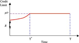
Figure 14 Optimal credit limit, as a function of time.
This model illustrates how the distortions due to adverse selection disappear over time. The credit available to the agent is initially restricted due to adverse selection, but the credit limit rises over time, and from time T onwards the optimal contract looks as if adverse selection were never a problem. The agent is initially in a “hot seat”. A shorter credit limit is unforgiving about losses. As a result, if the agent could affect the cash flows with effort, he would work harder up front to differentiate himself from types with a bad project.
The solution of Garrett and Pavan (2009) illustrates a similar pattern using a model that is different in many ways. One major difference from Sannikov (2007) is that the absence of adverse selection leads to a first-best outcome in the model of Garrett and Pavan (2009), as the agent is risk-neutral and does not have limited liability. Thus, the form of the optimal contract converges to first-best over time.
Several other papers have explored dynamic contracts in settings with asymmetric information. For example, Tchistyi (2006) and DeMarzo and Sannikov (2010) investigate settings where the firm’s cash flows are correlated over time. Thus, the agent has private information about the distribution of future cash flows (at least off the equilibrium path). Williams (2011) and Kwon (2012) also address the issues of persistence, and Golosov, Troshkin, and Tsyvinsky (2010) as well as Farhi and Werning (2011) focus on these issues in the context of public finance. While several common themes emerge, in general there is no unified way to analyze settings of dynamic adverse selection and moral hazard, and this area is ripe for future research.
References
1. Abreu D, Pearce D, Stacchetti E. Toward a theory of discounted repeated games with imperfect monitoring. Econometrica. 1990;58:1041–1063.
2. Albuquerque R, Hopenhayn HA. Optimal lending contracts and firm dynamics. Review of Economic Studies. 2004;72(2):285–315 No. 247.
3. Baker M, Wurgler J. Market timing and capital structure. Journal of Finance. 2002;57(1):1–32.
4. Bernanke B, Gertler M, Gilchrist S. The financial accelerator in a quantitative business cycle framework. In: Elsevier 1999:1341–1393. Taylor JB, Woodford M, eds. Handbook of Macroeconomics. Vol. 1 chap. 21.
5. Bernanke BS, Gertler M. Agency costs, net worth, and business fluctuations. American Economic Review. 1989;79(1):14–31.
6. Biais B, Mariotti T, Plantin G, Rochet J-C. Dynamic security design: Convergence to continuous time and asset pricing implications. Review of Economic Studies. 2007;74(2):345–390.
7. Biais B, Mariotti T, Rochet J-C, Villeneuve S. Large risks, limited liability and dynamic moral hazard. Econometrica. 2010;78(1):73–118.
8. Black F, Cox J. Valuing corporate securities: Some effects of bond indenture provisions. Journal of Finance. 1976;31:351–367.
9. Bolton P, Chen H, Wang N. A unified theory of Tobin’s q, corporate investment, financing and risk management. Journal of Finance. 2011;66(5):1545–1578.
10. Bolton, P., Chen, H., & Wang, N. (2012). Market timing, investment and risk management. Working paper, Columbia University.
11. Bolton P, Sharfstein D. A theory of predation based on agency problems in financial contracting. American Economic Review. 1990;80(1):93–106.
12. Brunnermeier, M., & Sannikov, Y. (2011). A macroeconomic model with a financial sector. Working paper, Princeton University.
13. Clementi GL, Hopenhayn H. A theory of financing constraints and firm dynamics. Quarterly Journal of Economics. 2006;121(1):229–265.
14. Daley, B., & Green, B. (2012). Asset trading, news and liquidity in markets with asymmetric information. Working paper, Princeton University.
15. Daley, B., & Green, B. (2012). Waiting for news in the market for lemons. Econometrica. 80(4), 1433–1504.
16. DeMarzo P, Duffie D. A liquidity-based model of security design. Econometrica. 1999;97(1):65–100.
17. DeMarzo P, Fishman M. Optimal long-term financial contracting. Review of Financial Studies. 2007a;20:2079–2128.
18. DeMarzo P, Fishman M. Agency and optimal investment dynamics. Review of Financial Studies. 2007b;20:151–188.
19. DeMarzo, P., Fishman, M., He, Z., & Wang, N. (2011). Dynamic agency and the q theory of investment. Working paper, Stanford GSB.
20. DeMarzo, P., Livdan, D., & Tchistyi, A. (2012). Risking other people’s money: Gambling, limited liability and optimal incentives. Working paper, UC Berkeley.
21. DeMarzo P, Sannikov Y. Optimal security design and dynamic capital structure in a continuous-time agency model. Journal of Finance. 2006;61:2681–2724.
22. DeMarzo, P., & Sannikov, Y. (2010). Learning, termination, and payout policy in dynamic incentive contracts. Working paper, UC Berkeley.
23. Farhi, E., & Werning, I. (2011). Insurance and taxation over the life cycle. Working paper, Harvard University.
24. Gale D, Hellwig M. Incentive-compatible debt contracts: The one-period problem. Review of Economic Studies. 1985;52(4):647–663.
25. Garrett, D., & Pavan, A. (2009). Dynamic managerial compensation: A mechanism design approach. Working paper, Northwestern University.
26. Goldstein R, Ju N, Leland H. An EBIT-based model of dynamic capital structure. Journal of Business. 2001;74(4):483–512.
27. Golosov, M., Troshkin, M., & Tsyvinsky, A. (2010). Optimal dynamic taxes. Working paper, Princeton University.
28. Green EJ. Lending and the smoothing of uninsurable income. In: Prescott EC, Wallace N, eds. Contractual arrangements for intertemporal trade. University of Minnesota Press 1987.
29. Hayashi F. Tobin’s q, and average q: A neoclassical interpretation. Econometrica. 1982;50:215–224.
30. He Z. Optimal executive compensation when firm size follows geometric Brownian motion. Review of Financial Studies. 2009;22(2):859–892.
31. He, Z., & Krishnamurthy, A. (2012). A model of capital and crises. Working paper, Northwestern University.
32. Hennessy, C., Livdan, D., & Miranda, B. (2008). Repeated signaling and firm dynamics. Working paper, Northwestern University.
33. Hoffmann F, Pfeil S. Reward for luck in a dynamic agency model. Review of Financial Studies. 2010;23(9):3329–3345.
34. Holmstrom B. Managerial incentive problems – A dynamic perspective. Review of Economic Studies. 1999;66.
35. Holmstrom B, Milgrom P. Multitask principal-agent analyses: Incentive contracts, asset ownership, and job design. Journal of Law, Economics, and Organization. 1991;7:24–52.
36. Jensen M, Meckling W. Theory of the firm: Managerial behavior, agency costs and ownership structure. Journal of Financial Economics. 1976;3:305–360.
37. Kwon, S. (2012). Dynamic moral hazard with persistent states. Working paper, MIT.
38. Leland H. Corporate debt value, bond covenants and optimal capital structure. Journal of Finance. 1994;49(4):1213–1252.
39. Leland H, Pyle D. Informational asymmetries, financial structure and financial intermediation. Journal of Finance. 1977;32(2):371–387.
40. Lucas D, McDonald R. Equity issues and stock price dynamics. Journal of Finance. 1990;45(4):1019–1043.
41. Modigliani F, Miller M. The cost of capital, financial structure and financial intermediation. American Economic Review. 1958;48(3):261–297.
42. Merton RC. The pricing of corporate debt: the risk structure of interest rates. Journal of Finance. 1974;29(2):449–470.
43. Myers S, Majluf N. Corporate financing and investment decisions when firms have information that investors do not have. Journal of Financial Economics 1984.
44. Myerson R. Incentive compatibility and the bargaining problem. Econometrica. 1979;47(1):61–74.
45. Pavan, A., Segal, I., & Toikka, J. (2009). Dynamic mechanism design: Incentive compatibility, profit maximization and information disclosure. Working paper, Stanford University.
46. Phelan C, Townsend R. Computing multi-period, information-constrained optima. Review of Economic Studies. 1991;58:853–881.
47. Piskorski T, Tchistyi A. Optimal mortgage design. Review of Financial Studies. 2010;23(8):3098–3140.
48. Radner R. Repeated principal-agent games with discounting. Econometrica. 1985;53:1173–1198.
49. Rampini, A., & Vishwanathan, S. (2012). Collateral and capital structure. Working paper, Duke University.
50. Rampini A, Vishwanathan S. Collateral, risk management and the distribution of debt capacity. Journal of Finance. 2010;65:2293–2322.
51. Rogerson WP. Repeated moral hazard. Econometrica. 1985;53:69–76.
52. Sannikov, Y. (2007). Agency problems, screening and increasing credit lines. Working paper, University of California at Berkeley.
53. Sannikov Y. A continuous-time version of the principal-agent problem. Review of Economic Studies. 2008;75:957–984.
54. Spear S, Srivastava S. On repeated moral hazard with discounting. Review of Economic Studies. 1987;54:599–617.
55. Tchistyi, A. (2006). Security design with correlated hidden cash flows: The optimality of performance pricing. Working paper, UC Berkeley.
56. Townsend R. Optimal contracts and competitive markets with costly state verification. Journal of Economic Theory. 1979;21(2):265–293.
57. Williams N. Persistent private information. Econometrica 2011.
58. Zhu, J. (2011). Sticky incentives and dynamic agency: Optimal contracting with perks and shirking. Working paper, UC Berkeley.
*I am most grateful to Milton Harris for his generous guidance and extensive suggestions during the preparation of this manuscript. I would also like to thank Neng Wang, Brett Green, Brendan Daley, Alexei Tchistyi, and Thomas Mariotti for helpful comments.
1However, when tax advantages of debt exist, then the overall cost of capital can easily increase with stricter constraints on leverage.
2This point is developed in the dynamic model of DeMarzo, Fishman, He, and Wang (2011) that we discuss in Section 4. In that model, the scale of investment varies dynamically with the agents’ wealth, which itself depends on the firm’s past performance.
3While the amount of debt is fixed at time 0 in the model of Leland (1994), Goldstein, Ju, and Leland (2001) provide an important extension in which the firm has an option to increase the level of debt, but cannot decrease it.
4If not, then two solutions of (6), F and ![]() such that
such that ![]() would have the same slope
would have the same slope ![]() at some point W > R. Take the lowest such W. Then
at some point W > R. Take the lowest such W. Then ![]() and for all
and for all ![]() and so
and so ![]() . However, then Eq. (6) implies that
. However, then Eq. (6) implies that ![]() , so
, so ![]() for some small ɛ > 0, a contradiction.
for some small ɛ > 0, a contradiction.
5Note also that a single choice of ![]() is optimal for all values of W0.
is optimal for all values of W0.
6If ![]() , then the cash inflows that reduce the agent’s credit line balance can be interpreted as interest payments from a compensating balance that the agent holds with the principal, in order to access a particularly long (in this case) credit line.
, then the cash inflows that reduce the agent’s credit line balance can be interpreted as interest payments from a compensating balance that the agent holds with the principal, in order to access a particularly long (in this case) credit line.
7DFHW incorporate adjustment costs in the firm’s capital accumulation equation in a way that is different from, but equivalent to, the form presented here. Specifically, they model the firm’s investment technology in the form dKt = (It − δKt)dt and the cash flows in the form dXt = Kt(dYt − c(It/Kt)dt) − It dt, where c is a convex adjustment cost function. The two formulations are equivalent: they present two ways of describing the firm’s production set of expected output and new capital, per unit of existing capital. The production set is (atμ − c(i) − i, i − δ) under the formulation of DFHW, and (atμ − ι, Φ(ι) − δ) under the formulation we work with above.
8Hoffmann and Pfeil (2010) assume instead that the mean of cash flows may experience only a one-time jump up (good luck) or down (bad luck).
9Section 6 in DeMarzo et al. (2011) independently makes the same point.
10In this model, unlike in DS and DFHW, the optimal contract exists even if the agent is equally patient as the principal.
11Note that Φ can be negative, i.e. it is possible to destroy capital, but ![]() cannot be negative, i.e. the destruction of capital does not generate any liquidating cash flows.
cannot be negative, i.e. the destruction of capital does not generate any liquidating cash flows.
12This issue arises also in discrete-time principal-agent models, e.g. see DeMarzo and Fishman (2007a, 2007b). It is absent from Brownian models, or Poisson models in which jumps are “good news”.
13A recent paper of DeMarzo, Livdan, and Tchistyi (2012) builds upon the modeling elements of DS and BMRV to study optimal contracting in settings where managers can take hidden tail risks to boost perceived returns. They find that in the optimal contract, managers take more tail risks after poor performance, when they have less “skin in the game”.
14Holmstrom, (1999) provides a linear dynamic model with static wage contracts, which illustrates how signaling incentives on the degree of uncertainty.
15Daley and Green (2012b) relax this assumption and endogenize the value of the asset to the purchaser, as the purchaser may need to trade the asset in the future due to liquidity shocks.
16Thus, dzt = (μH − μL)2/(2σ2)dt + (μH − μL)/σ dZt conditional on type H, and dzt = −(μH − μL)2/(2σ2)dt + (μH − μL)/σ dZt conditional on type L.
17Recall that on the equilibrium path, process Qt is non-decreasing because no trade is good news about the type of the seller.
18In general, adverse selection problems alone can be solved very effectively via state-contingent dynamic contracts, and interesting frictions arise only when moral hazard is also present. In practice, it is difficult to imagine a situation where adverse selection exists by itself without moral hazard.
19If the agent is risk-neutral and has the same discount rate as the principal, it is optimal to postpone payments to the agent indefinitely, or until the time when the contract is first-best. We have already encountered this fact in the model of He (2009).