
Chapter 3
Do Taxes Affect Corporate Decisions? A Review
Abstract
Keywords
Taxes; Corporate taxation; Capital structure; Corporate finance; Compensation; Dividends; Payout policy
1 Introduction
Taxes are thought to affect corporate decisions in important ways. Witness the numerous changes the US government has made (or has considered making) to the tax code to affect corporate behavior. Just in the past decade: (1) Equity tax rates have been reduced for retail investors in an attempt to reduce the corporate cost of capital, and these changes are thought to have altered corporate payout policy. (2) During the last two recessions, in an attempt to stimulate the corporate sector, the government has temporarily granted companies the ability to carry current period losses back five years, to receive a refund on any taxes paid during the past five years. (3) Companies have been temporarily granted the ability to deduct depreciation at an accelerated rate, and earn a tax credit for research and development spending, to encourage corporate spending. (4) President Obama’s administration and European authorities are considering whether to eliminate or reduce the ability of companies to deduct interest payments from taxable income, because allegedly this tax-favored status of debt has encouraged too much debt financing, thereby exacerbating economic downturns. (5) There have been proposals to reduce the top US corporate income tax rate from 35% to approximately 25%, in an effort to make US firms more competitive and also to reduce distortions caused by income taxes. One such distortion occurs when US multinationals park large quantities of cash overseas to avoid paying repatriation taxes that would be incurred if the US parent were to bring the foreign profits back home. These examples make it clear that taxes play an important role in public policy and political debates. The focus of this chapter, however, is not public policy. Rather, this chapter takes the tax rules as given and focuses on how corporate choices and actions are affected by the incentives provided by them. In this paper, I review academic research related to many different tax issues, with the goal of providing a better understanding of when taxes appear to have a first-order effect on corporate behavior, versus when taxes do not appear to have much if any effect on corporate actions.
Modigliani and Miller (1958) and Miller and Modigliani (1961) lay the groundwork for analyzing whether taxes matter. Modigliani and Miller (MM) assume that capital markets are perfect, which implies that there are no corporate or personal taxes, among other things. They demonstrate that corporate financial decisions are irrelevant in a perfect, taxless world. During the past 45 years, research has studied how financial decisions become relevant as the perfect capital markets assumptions are relaxed. The research reviewed in this chapter investigates the consequences of the existence of imperfections related to corporate and personal taxation, highlighting the role of corporate and investor taxes in corporate policies and firm value.1 This role is potentially very important, given the sizable tax rates that many corporations and individuals face (see Figure 1).

Figure 1 Corporate and personal income tax rates. The highest tax bracket statutory rates are shown for individuals and C-corporations. The corporate capital gains tax rate (not shown) was equal to the corporate income tax rate every year after 1987. In May 2003, President Bush signed into law a reduction in the top personal income tax rate to 35% in 2003. This same law reduced top personal tax rates on capital gains and dividends to 15%. In late 2010, President Obama and Congress agreed to keep the personal tax rates in place through 2012 and to revisit the issue later, and the Bowles–Simpson commission recommended a reduction in the corporate income tax rate to 25%. Thus, as this chapter goes to press, it seems quite possible that personal and corporate income tax rates will change in the near future.
Modigliani and Miller argue that corporate financial policies do not add value in equilibrium, and therefore firm value equals the present value of operating cash flows. Once imperfections are introduced, however, corporate financial policies can affect firm value, and firms should pursue a given policy until the marginal benefit of doing so equals the marginal cost. A common theme in tax research involves expressing how various tax rules and regulations affect the marginal benefit of corporate actions. For example, when tax rules allow interest deductibility, a $1 interest deduction provides tax savings of $1 × τC(.). The function τC(.) measures corporate marginal tax benefits and is conditional on statutory tax rates, nondebt tax shields, the probability of experiencing a loss, international tax rules about dividend imputation and interest allocation, organizational form, and various other tax rules. A common theme that runs throughout this chapter is to describe how various tax rules affect the τC(.) benefit function, and therefore how they affect corporate incentives and decisions. A second but less common theme is related to how market imperfections affect tax costs. Given that this chapter reviews tax research, the emphasis is on research that describes how taxes affect costs and benefits—and the influence of nontax factors is discussed only briefly.
There are multiple avenues for taxes to affect corporate decisions. As outlined in the Table of Contents, taxes can affect capital structure decisions, both domestic (Section 2) and multinational (Section 3), organizational form and restructurings (Section 4), payout policy (Section 5), compensation policy (Section 6), risk management (Section 7), and the use of tax shelters (Section 8). For each of these areas, a brief theoretical framework is presented that describes how taxes might affect corporate decisions, followed by empirical predictions based on the theory and summaries of the related empirical evidence. This approach seeks to highlight important questions about how taxes affect corporate decisions, and to summarize and, in some cases, critique the answers that have been thus far provided. Each section concludes with a discussion of unanswered questions and possible avenues for future research. Overall, substantial progress has been made in the investigation of whether and how taxes affect corporate financial decisions, but much work remains. Section 9 concludes and proposes directions for future research.
2 Taxes and Capital Structure—The US Tax System
2.1 Theory and Empirical Predictions
This section reviews capital structure research that is related to the “classical” tax system found in the United States. (Section 3 reviews multinational and imputation tax systems.) The key features of the classical system are that corporate income is taxed at a rate τC, interest is deductible and so is paid out of income before taxes, and equity payout is not deductible but is paid from the residual remaining after corporate taxation. In this tax system, interest, dividends, and capital gains income are taxed upon receipt by investors (at tax rates τP, τdiv, and τG, respectively). Most research assumes that equity is the marginal source of funds and that dividends are paid according to a fixed payout policy.2 To narrow the discussion, assume that regulations or transactions costs prevent investors from following the tax-avoidance schemes implied by Miller and Scholes (1978), in which investors borrow via insurance or other tax-free vehicles to avoid personal tax on interest or dividend income.
In this framework, the after-personal-tax value to investors of a corporation paying $1 of interest is $1(1 − τP). In contrast, if that capital were instead returned as equity income, it would be subject to “double taxation” and would be taxed at both the corporate and personal level; the equity investor would receive $1(1 − τC)(1 − τE). The equity tax rate, τE, is often modeled as a blended dividend and capital gains tax rate.3 The net tax advantage of $1 of debt payout, relative to $1 of equity payout, is
![]() (1)
(1)
If Eqn (1) is positive, debt interest is the tax-favored way to return capital to investors, once both corporate and individual taxation are considered. In this case, in order to maximize firm value, a company has a tax incentive to issue debt instead of equity.
Equation (1) captures the benefit of a firm paying out $1 as debt interest in the current period, relative to paying out $1 as equity income. If a firm has $D of debt with coupon rate rD, the net benefit of using debt rather than equity is
![]() (2)
(2)
Given this expression, the value of a firm with debt can be written as
![]() (3)
(3)
where the PV term measures the present value of all current and future interest deductions. Note that Eqn (3) implicitly assumes that using debt adds tax benefits but has no other effect on incentives, operations, or value. In particular, (3) ignores all capital structure costs other than possible personal tax costs.4 The expression also assumes, a la MM, that there are no feedback effects from capital structure on operating decisions (e.g. no debt-induced agency costs).
The Modigliani and Miller (1958) set-up is the starting point for capital structure research. If capital markets are perfect, τC, τP, and τE all equal zero, and firm value is not affected by whether the firm finances with debt or equity (i.e., Valuewith debt = Valueno debt). That is, the value of the firm equals the value of equity plus the value of debt, but total value is not affected by the proportions of debt and equity. This implication is used as the null throughout the capital structure discussion.
Null hypotheses: Firms do not have optimal tax-driven capital structures.
The value of a firm with debt is equal to the value of an identical firm without debt (i.e., there is no net tax advantage to debt).
In their “correction article”, MM (1963) consider corporate income taxation but continue to assume that τP and τE equal zero. In this case, the second term in Eqn (3) collapses to PV[τCrDD]: Because interest is deductible, paying $rDD of interest saves τCrDD in taxes each period relative to returning capital as equity. MM (1963) assume that debt is fixed and hence that interest deductions are as risky as the debt that generates them and should be discounted by rD.5 With perpetual debt, MM (1963) argue that the value of a firm with debt financing is:
![]() (4)
(4)
where the τCD term represents the tax advantage of debt. Note that Eqn (4) contains a term that captures the tax benefit of using debt (τCD) but no offsetting cost of debt term. Eqn (4) has two strong implications. First, corporations should finance with 100% debt because the marginal benefit of debt is τC, which is usually assumed to be a positive constant. Second, if τC is constant, firm value increases (linearly) with D due to tax benefits.
The first implication was recognized as extreme, and researchers soon developed models that relax the MM (1958) assumptions and consider costs of debt. In the early models, firms trade off the tax benefits of debt with costs. The first cost proposed in the literature was the cost of bankruptcy, or more generally, costs of financial distress. Kraus and Litzenberger (1973), using a state-preference framework, show that firms should trade off bankruptcy costs with the tax benefits of debt to arrive at an optimal capital structure that involves less than 100% debt. Scott (1976) shows the same thing with continuous variables. For decades, the bankruptcy cost solution was viewed as not large enough empirically in magnitude to ex ante offset the benefits of debt.6 Therefore, other papers proposed nonbankruptcy costs that could be traded off against the tax benefits of debt. For example, Jensen and Meckling (1976) introduce agency costs of equity and leverage-related deadweight costs.7Myers (1977) introduces underinvestment costs that can result from too much debt.8
Regardless of the type of cost, the basic trade-off implications remain similar to those in MM (1963): (1) the incentive to finance with debt increases with the corporate tax rate, and (2) firm value increases with the use of debt (up to the point where the marginal cost equals the marginal benefit of debt). Note also that in these models, different firms can have different optimal debt ratios depending on the relative costs and benefits of debt (i.e. depending on differing firm characteristics).
Prediction 1: All else constant, for taxable firms, value increases with the use of debt because of tax benefits (up to the point where the marginal cost equals the marginal benefit of debt).
Prediction 2: Corporations have a tax incentive to finance with debt that increases with the corporate marginal tax rate. All else equal, this implies that firms have different optimal debt ratios to the extent that their tax rates differ.
Prediction 1 is based directly on Eqn (4), whereas Prediction 2 is based on the first derivative of Eqn (4) with respect to D.
Miller (1977) argues that personal taxes can eliminate the “100% debt” implication, without the need for bankruptcy or agency costs. (Farrar and Selwyn, 1967, took first steps in this direction.) Miller’s argument is that the marginal costs of debt and equity, net of the effects of personal and corporate taxes, should be equal in equilibrium, so firms are indifferent between the two financing sources. In essence, the corporate tax savings from debt are offset by the personal tax disadvantage to investors from holding debt, relative to holding equity. All else equal (including risk), this personal tax disadvantage causes investors to demand higher pretax returns on debt, relative to equity returns. From the firm’s perspective, paying this higher pretax return wipes out the tax advantage of using debt financing.
Figure 2 illustrates Miller’s point. (Note that Figure 2 has the tax benefit savings from a dollar of interest (measured as τC) on the y-axis, rather than returns as in Miller (1977).) The horizontal line in Panel A depicts the supply curve for debt; the line is horizontal because Miller assumes that the benefit of debt for all firms equals a fixed constant τC. The demand for debt curve is initially horizontal at zero, representing demand by tax-free investors, but eventually slopes upward because the return on debt must increase to attract investors with higher personal income tax rates. By making the simplifying assumption that τE = 0, Miller’s equilibrium is reached when the marginal investor with ![]() is attracted to purchase debt. In equilibrium, the overall amount of debt supplied by firms equals aggregate demand by investors. In this equilibrium, the entire surplus (the area between the supply and demand curves) accrues to investors subject to personal tax rates less than τP*.
is attracted to purchase debt. In equilibrium, the overall amount of debt supplied by firms equals aggregate demand by investors. In this equilibrium, the entire surplus (the area between the supply and demand curves) accrues to investors subject to personal tax rates less than τP*.
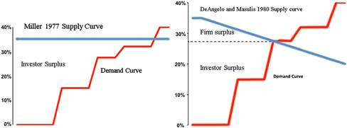
Figure 2 Equilibrium supply and demand curves for corporate debt. The supply curve shows the expected tax rate (and therefore the tax benefit of a dollar of interest) for the firms that issue debt. The demand curve shows the tax rate (and therefore the tax cost of a dollar of interest) for the investors that purchase debt. The tax rates for the marginal supplier of and investor in debt are determined by the intersection of the two curves. In the Miller Equilibrium (panel A), all firms have the same tax rate in every state of nature, so the supply curve is flat. The demand curve slopes upward because tax-free investors are the initial purchasers of corporate bonds, followed by low-tax-rate investors, and eventually followed by high tax-rate-investors. In the Miller Equilibrium, all investors with tax rates less than the marginal investor’s (i.e., investors with tax rates of 35% or less in Panel A) are inframarginal and enjoy an “investor surplus” in the form of an after-tax return on debt higher than their reservation return. In Panel B, the supply curve is downward sloping because firms differ in terms of the probability that they can fully utilize interest deductions (or have varying amounts of nondebt tax shields), and therefore have differing benefits of interest deductibility. Firms with tax rates higher than that for the marginal supplier of debt (i.e., firms with tax rates greater than 28% in Panel B) are inframarginal and enjoy “firm surplus” because the benefit of interest deductibility is larger than the personal tax cost implicit in the debt interest rate Panel A.
Miller’s (1977) analysis has several implications. The first two are not reflected in Predictions 1 or 2:
Prediction 3: High personal taxes on interest income (relative to personal taxes on equity income) create a disincentive for firms to use debt.
Prediction 4: The aggregate supply of debt is affected by relative corporate and personal taxes.
The other implications are consistent with the null hypotheses stated above: (1) there is no net tax advantage to debt at the corporate level (once one accounts for the higher debt yields investors demand because of the relatively high personal taxes associated with receiving interest), (2) though taxes affect the aggregate supply of debt in equilibrium, they do not affect the optimal capital structure for any particular firm (i.e. it does not matter which particular firms issue debt, as long as aggregate supply equals aggregate demand), and (3) using debt does not increase firm value.
A general version of the Miller argument (that does not assume τE = 0) can be expressed analogously to Eqn (4) with perpetual debt. Once personal taxes are introduced into this framework, the appropriate discount rate is measured after personal income taxes to capture the (after-personal-tax) opportunity cost of investing in debt. In this case, the value of a firm using perpetual debt is, where rD is the before-personal-tax expected rate of return on debt investors require 9:
![]() (5)
(5)
If the investor-level tax on interest income (τP) is large relative to tax rates on corporate and equity income (τC and τE), the net tax advantage of debt can be zero or even negative. Note that Eqn (5) is identical to Eqn (4) if there are no personal taxes, or if τP = τE.
One way that Eqn (5) can be an equilibrium expression is for the rightmost term in this equation to equal zero in equilibrium (e.g. (1 − τP) = (1 − τC)(1 − τE)), in which case the implications from Miller (1977) are unchanged. Alternatively, the tax benefit expressed in the bracketed term in Eqn (5) can be positive, and a separate cost term can be introduced in the spirit of the trade-off models. In this case, the corporate incentive to issue debt and firm value both increase with [1 − (1 − τC)(1 − τE)/(1 − τP)] and firm-specific optimal debt ratios can exist. The bracketed expression specifies the degree to which personal taxes (Prediction 3) offset the corporate incentive to use debt (Prediction 2). Recall that τP and τE are personal tax rates for the marginal investor(s) (i.e. price-setters) and therefore are very difficult to pin down empirically (more on this in Section 2.4).
DeAngelo and Masulis (1980; hereafter DM) broaden Miller’s (1977) model and put the focus on the marginal tax benefit of debt, represented earlier by τC. The DM argument focuses on nondebt tax shields (NDTS) and can be nested within an argument that τC(.) is not constant and is therefore not always equal to the statutory rate. In particular, τC(.) is a decreasing function of nondebt tax shields (e.g. depreciation and investment tax credits) because NDTS crowd out the tax benefit of interest. Furthermore, Kim (1989) highlights the fact that firms do not always benefit fully from incremental interest deductions because they are not taxed when taxable income is negative. Extending this logic implies that τC(.) is a decreasing function of a firm’s debt usage because existing interest deductions crowd out the tax benefit of incremental interest.
Modeling τC(.) as a function, rather than a constant equal to the statutory tax rate, has important implications because the supply of debt function becomes downward sloping (see Panel B in Figure 2). This implies that using debt has a corporate advantage, as measured by the “firm surplus” of issuing debt (the area above the dotted line but below the supply curve in Panel B). Moreover, high-tax-rate firms supply debt (i.e. are on the portion of the supply curve to the left of its intersection with demand), which implies that tax-driven firm-specific optimal debt ratios can exist (as in Prediction 2), and that the tax benefits of debt add value for high-tax-rate firms (as in Prediction 1). The DeAngelo and Masulis (1980) approach leads to the following prediction, which essentially expands Prediction 2:
Prediction 2’: All else equal, to the extent that they reduce τC(.), nondebt tax shields and/or interest deductions from already-existing debt reduce the tax incentive to use debt. Similarly, the tax incentive to use debt decreases with the probability that a firm will experience nontaxable states of the world.
2.2 Empirical Evidence on Whether the Tax Advantage of Debt Increases Firm Value
Prediction 1 indicates that the tax benefits of debt add τCD (Eqn (4)) or [1 − (1 − τC)(1 − τE)/(1 − τP)]D (Eqn (5)) to firm value. If τC = 40% and the debt ratio is 35%, Eqn (4) indicates that the contribution of taxes to firm value equals 14% (0.14 = τC × debt-to-value). This calculation is an upper bound, however, because it ignores costs and other factors that reduce the corporate tax benefit of interest deductibility, such as personal taxes, nontax costs of debt, and the possibility that interest deductions are not fully valued in every state of the world. This section reviews empirical research that attempts to quantify the net tax benefits of debt. The first group of papers studies market reactions to exchange offers, which should net out the various costs and benefits of debt. Then, recent analyses based on large-sample regressions are reviewed. The section concludes by examining explicit calculation of benefit functions for interest deductions.
2.2.1 Exchange Offers
To investigate whether the tax benefits of debt increase firm value (Prediction 1), Masulis (1980) examines exchange offers made during the 1960s and 1970s. Because one security is issued and another is simultaneously retired in an exchange offer, Masulis argues that exchanges hold investment policy relatively constant and are primarily changes in capital structure. Masulis’s tax hypothesis is that leverage increasing (decreasing) exchange offers increase (decrease) firm value because they increase (decrease) tax deductions. Note that Masulis implicitly assumes that firms are underlevered and that the exchange announcement is unanticipated. For a company already at its optimum, a movement in either direction (i.e. increasing or decreasing debt) would decrease firm value.
Masulis (1980) finds evidence consistent with his predictions: leverage-increasing exchange offers increase equity value by 7.6%, and leverage-decreasing transactions decrease by 5.4%. Moreover, the exchange offers with the largest increases in tax deductions (debt-for-common and debt-for-preferred) have the largest positive stock price reactions (9.8% and 4.7%, respectively). Using a similar sample, Masulis (1983) regresses stock returns on the change in debt in exchange offers and finds a debt coefficient of approximately 0.40 (which is statistically indistinguishable from the top statutory corporate tax rate during that era). This is consistent with taxes increasing firm value as in Eqn (4) (and is also consistent with some alternative hypotheses discussed below), but it is surprising because such a large coefficient implies near-zero personal tax and other costs to debt and/or large nontax benefits to debt. That is, the debt coefficient in Masulis (1983) measures the average benefit of debt (averaged across firms and averaged over the incremental net benefit of each dollar of debt for a given firm) net of the costs. An average net benefit of 0.40 requires that the costs are much smaller than the benefits for most dollars of debt. For the post-exchange offer capital structure to satisfy the MB = MC equilibrium condition, and given that the average benefit is approximately equal to the maximum statutory tax rate, the benefit or cost curve (or both) must be very steeply sloped near their intersection.
Myers (1984) and Cornett and Travlos (1989) argue that Masulis’s (1980) hypothesis is problematic. If firms optimize, they should only adjust capital structure to move toward an optimal debt ratio, whether that involves increasing debt or equity. In other words, increasing debt will not always add to firm value, even if interest reduces tax liabilities. Graham, Hughson, and Zender (1999) point out that if a firm starts at its optimal capital structure, it will only perform an exchange offer if something moves the firm out of equilibrium. They derive conditions under which stock price-maximizing exchanges are unrelated to marginal tax rates because market reactions aggregate tax and nontax informational aspects of capital structure changes. Therefore, nontax reactions might explain Masulis’s (1980) results. As described next, several papers have found evidence of nontax factors affecting exchange offer market reactions. It is important to note that these post-Masulis papers do not prove that the tax interpretation is wrong—but they do offer reasonable alternative interpretations.
First, some papers find evidence of positive (negative) stock reactions to leverage-increasing (leverage-decreasing) events that are unrelated to tax deductions: Asquith and Mullins (1986), Masulis and Korwar (1986), and Mikkelson and Partch (1986) find negative stock price reactions to straight equity issuance, and Pinegar and Lease (1986) find positive stock price reactions to preferred-for-common exchanges. Second, Mikkelson and Partch (1986) and Eckbo (1986) report that straight debt issuance (without equity retirement) produces a stock price reaction that is indistinguishable from zero. Third, some papers find that exchange offers convey nontax information that affects security prices, perhaps due to asymmetric information problems along the lines suggested by Myers and Majluf (1984) or due to signaling (Leland and Pyle, 1977; Ross, 1977). For example, Shah (1994) correlates exchange offers with information about reduced future cash flows (for leverage-decreasing offers) and decreased risk (for leverage-increasing offers). Finally, Cornett and Travlos (1989) provide evidence that weakens Masulis’s (1983) conclusions. Cornett and Travlos regress stock returns around the exchange event on the change in debt and two variables that control for information effects (the ex-post change in inside ownership and ex-post abnormal earnings). They find that the coefficient on the change in debt variable is insignificant while the coefficients on the other variables are significant, which implies that the positive stock price reaction is related to positive information conveyed by the exchange.10 Cornett and Travlos conclude that equity-for-debt exchanges convey information about the future—but find no evidence of increased value due to tax benefits.
Two papers examine the exchange of traditional preferred stock for trust preferred stock, also known as monthly income preferred stock (MIPS). These two securities differ primarily in terms of their tax characteristics, so any market reaction should have minimal nontax explanations. MIPS interest is tax deductible for corporations (like debt interest), and preferred dividends are not. On the investor side, corporate investors enjoy a 70% dividends received deduction (DRD) for preferred dividends, but recipients of MIPS interest receive no parallel deduction.11 When issuing MIPS to retire preferred, corporations gain the tax benefit of interest deductibility but experience two costs: underwriting costs and possibly an increased coupon due to the personal tax penalty (because investors are fully taxed on MIPS interest in contrast to corporate investors, who receive the DRD on preferred dividends). Engel, Erickson, and Maydew (1999) compare MIPS yields to preferred yields and conclude that the tax benefits of MIPS are approximately $0.28 per dollar of face value, net of costs. Irvine and Rosenfeld (2000) use abnormal announcement returns to estimate the value at $0.26. Given that MIPS and preferred are nearly identical in all legal and informational respects, these studies provide straightforward evidence of the positive effect of interest tax deductions at the corporate level on firm value, net of underwriting and personal tax costs. Given that the maximum tax benefit was 34% during the sample period, and average benefits are about $0.27 according to these studies, the results imply that the non-bankruptcy costs of debt financing (including personal tax costs) are only moderate. (Note that expected bankruptcy costs are similar between MIPS and traditional preferred, so do not affect the numbers mentioned above).
2.2.2 Cross-Sectional Regressions
Fama and French (1998; hereafter FF) attempt to estimate Eqn (4) and Prediction 1 directly, by regressing Vwith debt on debt interest, dividends, and a proxy for Vwithout debt. They argue that a positive coefficient on interest would be evidence of positive tax benefits of debt. FF measure Vwith debt as the excess of market value over book assets. They proxy Vwithout debt with a collection of control variables, including current earnings, assets, and R&D spending, as well as future changes in these same variables. (All the variables in the regression are deflated by assets.) If these control variables adequately proxy for Vwithout debt, the regression coefficient on interest will measure the net benefit of debt (which is hypothesized to be positive). A major difficulty with this approach is that if the control variables measure Vwithout debt with error, the regression coefficients can be biased. (Another difficulty is that if all firms choose optimal capital structures and operate at the maximum Vwith debt point, then one could not detect a causal empirical relation between value and debt usage. To detect causal relations between debt and value, one would require that a friction requires some firms to operate suboptimally).
FF perform a series of regressions on a broad cross-section of firms, using both level-form and first-difference specifications. In all cases, the coefficient on interest is either insignificant or negative. Fama and French interpret their results as being inconsistent with debt tax benefits having a first-order effect on firm value. Instead, they argue that interest provides information about earnings that is not otherwise captured by their controls for Vwithout debt. In other words, Vwithout debt is measured with error, which results in the interest coefficient picking up a negative valuation effect related to financial distress or some other cost.
Kemsley and Nissim (2002) attempt to circumvent this measurement problem. They perform a switch of variables, moving the earnings variable (which they assume proxies Vwithout debt with error) to the left-hand side of the regression and Vwith debt to the right side. Therefore, their regression tests the relation Vwithout debt = Vwith debt − coeff*D.
When Kemsley and Nissim regress earnings before interest and tax (EBIT) on Vwith debt and debt, the debt coefficient is negative, which they interpret as evidence that debt contributes to firm value. The coefficient also changes through time in conjunction with changes in statutory tax rates. The Kemsley and Nissim analysis should be interpreted carefully. First, their regression specification can be interpreted as measuring the effect of debt on earnings, just as well as it can be interpreted as a switch-of-variables that fixes a measurement error problem in Fama and French (1998). Second, the debt coefficient has the correct sign for the full sample only in a nonlinear specification in which all the right-hand side variables are interacted with a crude measure of the discount rate. Finally, the coefficient that measures the net benefit of debt has an absolute value of 0.40. While consistent with Masulis (1983), such a large coefficient implies near-zero average debt costs including a near-zero effect of personal taxes.
2.2.3 Marginal Tax Benefit Functions
Graham (2000, 2001) uses a third approach to estimate the contribution of debt interest deductibility to firm value. He simulates interest deduction marginal benefit functions and integrates under them to estimate the tax-reducing value of a given amount of interest expense. For a given level of interest deductions, Graham essentially averages over possible states of the world (i.e. both taxable and nontaxable states) to determine a firm’s expected τC, which specifies the expected tax benefit of an incremental dollar of interest deduction. Because this approach focuses on incremental interest deductions, in the context of incremental decisions this approach largely avoids the endogeneity problem described below in Section 2.3.3.
Marginal tax benefits of debt decline as more debt is added because the probability increases with each incremental dollar of interest that it will not be fully valued in every state of the world. Using simulation methods (described more fully in Section 2.3.2) and various levels of interest deductions, Graham maps out firm-specific interest benefit functions analogous to the supply of debt curve in Panel B of Figure 2.
Using this approach, Graham (2000) estimates that the tax benefit of debt equals approximately 9–10% of firm value during 1980–1994 (ignoring all costs). van Binsbergen et al. (2010) update these estimates and find that the gross tax benefits of debt averaged about 9.0% from 1995–2009. The fact that these figures are less than the 14% estimated (at the beginning of Section 2) with the back of the envelope “τCD” calculation reflects the reduced value of interest deductions in some states of the world. When personal taxes are considered, the tax benefit of debt falls to 7–8% of firm value during 1980–1994 (i.e. this is Graham’s estimate of the “firm surplus” in Panel B of Figure 2), meaning that the personal tax penalty reduces corporate tax benefits by about one-third. These averages are instructive but they mask that for some firms, the tax benefits of debt are even larger. van Binsbergen et al. (2010) sort by tax benefits and estimate that for the top decile of firms, gross tax benefits average about 25% of firm value, and for these firms tax benefits net of all costs average about 10%.
Graham (2000; his Figure 2) also estimates the “money left on the table” that firms could obtain if they levered up to the point where their last dollar of interest deduction is valued at the full statutory tax rate (i.e. the “kink” in the tax benefit function, which is the point just before incremental tax benefits begin to decline).12 The money left on the table calculations in Graham are partially updated in Table 1 of this paper. If all firms lever up to operate at the kink in their benefit functions, they could add 10.5% to firm value over the 1995–1999 period. This number can be interpreted (if many firms are underlevered) as a rough measure of the value loss due to conservative corporate debt policy, or (if most firms are optimally levered) as a lower bound for the difficult-to-measure costs of debt that would occur if a company were to lever up to its kink.
Table 1 Annual calculations of the mean benefits of debt and degree of debt conservatism. Before-financing MTR is the mean Graham (1996) simulated corporate marginal tax rate based on earnings before interest deductions, and after-financing MTR is the same based on earnings after interest deductions. Kink is the multiple by which interest payments could increase without a firm experiencing reduced marginal benefit on incremental deductions (i.e. the amount of interest at the point at which a firm’s marginal benefit function becomes downward sloping, divided by actual interest expense) as in Graham (2000). The tax benefit of debt is the reduction in corporate and state tax liabilities occurring because interest expense is tax deductible, expressed as a percentage of firm value. Money left on the table is the additional tax benefit that could be obtained, ignoring all costs, if firms with kink greater than one increased their interest deductions in proportion with kink.

This analysis initially yields two implications. First, the average unexploited tax benefits appear to be larger than the costs of debt that would occur if one were to lever up. Going back to Miller (1977) researchers have noted that the historic incidence of default is relatively low, meaning that the ex-ante probability of default is low. Interacting this low likelihood of default with ex-post measures of the cost of default (e.g. about 20% of firms value as in Andrade and Kaplan (1998)) implies expected costs of debt that on average appear to smaller than the forgone tax benefits. Almeida and Philippon (2007) point out the weakness of this logic. These authors highlight that distress most often occurs in bad states of the world, when the marginal utility of money is particularly high. Using credit default spreads to back out risk neutral probabilities that capture this effect, and using these risk neutral probabilities rather than historic incidence as their input into the expected cost of distress, Almeida and Philippon show that the expected cost of default approximately equals the “money left on the table” net of personal taxes estimate in Graham (2000), implying that firms on average may not be underlevered. This is an important point. One issue worth mentioning, perhaps, is that the Almeida and Philippon estimate of the personal tax costs, also used by Graham and others, is based on crude estimates. If this personal tax penalty happens to be overstated (e.g. if the marginal price-setter in the economy happens to be tax-free), then it is possible that the “underleverage” puzzle might not have been fully resolved by Almeida and Philippon.
The previous paragraph focuses on whether “on average” firms appear to be underlevered or not. The second implication of the money left on the table analysis is that cross sectionally the evidence seems to imply that the firms that appear to be conservative in their use of debt are large, profitable firms (which would seem to face the lowest costs of debt).13 This is puzzling because one would think that to forgo large tax benefits, a firm should face high expected costs of debt. In general, these implications are hard for a trade-off model to explain. There seem to be several possible explanations for this puzzle: (1) these firms that use debt conservatively do in fact face high costs but those costs have not been properly measured; (2) the apparent forgone tax benefits are overstated; (3) some firms are underlevered; and/or (4), the static trade-off model does not adequately explain debt policy. See Graham and Leary (2011) for a detailed examination of these issues. Briefly, I mention a couple points here.
Regarding (1), Graham (2000), Lemmon and Zender (2001) and Minton and Wruck (2001) try to identify nontax costs that are large enough in a trade-off sense that perhaps debt-conservative firms are not in fact underlevered. Blouin, Core, and Guay (2010) make some additional progress in identifying costs faced by apparently underlevered firms, though Graham and Kim (2009) argue that more evidence is needed to explain conservative debt policy. Regarding (2), it is important to emphasize that Graham’s (2000) tax benefit functions are calculated using financial statement data. Consequently, income or deductions that are “off balance sheet” may not be reflected in the income statement and therefore might not be captured in these tax benefit functions. This could result in financial statement income being overstated and hence potential tax benefits from levering up also being overstated.14Graham and Tucker (2006) gather data from 44 tax shelter legal filings and find that the annual deduction due to shelters is huge, averaging 9% of asset value. Given that these large deductions are not reflected in financial statement taxable income, these 44 companies had much less taxable income than was reflected in their financial statements, and hence the value gained from incremental interest deductions (i.e. apparent “money left on the table”) would also be less than estimated (because less “real” taxable income would mean that additional deductions in the form of interest would be less valuable). Similarly, Graham, Lang, and Shackleford (2004) hand-collect deductions occurring due to executive stock option exercises and find that these deductions are sizable, reducing taxable income for many firms and consequently reducing the tax benefits of incremental interest deductions. In both of these cases, firms that have substantial deductions that are not reflected in their financial statement filings would have smaller “tax benefits of debt” than would be estimated based on Graham’s financial-statement-based tax benefit functions. Therefore, researchers who do not incorporate deductions from off-balance sheet activity such as tax shelters and stock options may incorrectly conclude that a company uses too few interest deductions. Likewise, expenses associated with off-balance sheet pensions may have been missed by researchers attempting to measure taxable income using financial statements. It appears, however, that even after these special deductions are considered, the incremental tax benefits that could be obtained by issuing additional debt still appear to be fairly large. (One piece of good news: starting in reporting periods that end after June 2005, stock option deductions are now expensed, and hence financial statement income captures the effects measured by Graham, Lang, and Shackleford. Similarly, all pension expenses must now be reflected in the financial statements, so again, taxable income based on financial statement data should not be significantly flawed due to pension expense.)
To sum up, a fair amount of research has found evidence consistent with tax benefits adding to firm value. However, some of this evidence is ambiguous because nontax explanations or econometric issues cloud interpretation. Additional research in three specific areas would be helpful. First, we need more market-based research along the lines of the MIPS exchanges, where tax effects are isolated from information and other factors and therefore the interpretation is fairly unambiguous. Second, additional cross-sectional regression research that investigates the market value of the tax benefits of debt would be helpful in terms of clarifying or confirming the interpretation of existing cross-sectional regression analysis. Finally, if the tax benefits of debt do in fact add to firm value, an important unanswered question is why some firms do not use more debt, especially large, profitable firms.15 We need to better understand whether this implies that some firms are not optimizing, or whether previous research has not adequately modeled costs and other influences.
2.3 Empirical Evidence on Whether Corporate Taxes Affect Debt vs. Equity Policy
Trade-off models imply that firms should issue debt as long as the marginal benefit of doing so (measured by τC) is larger than the marginal cost. The benefit function τC(.) is a decreasing function of nondebt tax shields, existing debt tax shields, and the probability of experiencing losses, so the incentive to use debt declines with these three factors (Prediction 2’). In general, high-tax-rate firms should use more debt than low-tax-rate firms (Prediction 2). The papers reviewed in this section typically use reduced-form cross-sectional or panel regressions to test these predictions, and they ignore personal taxes altogether. For expositional reasons, we start with tests of Prediction 2’. Another set of papers (e.g. Hennessy and Whited, 2005) explore dynamic considerations more explicitly. These papers use structural models that use observed tax rates/incentives as an input, and study whether other observations about capital structure and investment match the empirical data. These models often find results that are consistent with observed data. Because this class of models only indirectly tests tax incentives, I do not review them herein. See Graham and Leary (2011) for more information.
2.3.1 Static Tax Rates
2.3.1.1 Nondebt Tax Shields (NDTS), Profitability, and the Use of Debt
Bradley, Jarrell, and Kim (1984) perform one of the early regression tests for tax effects along the lines suggested by DeAngelo and Masulis (1980). Bradley et al. regress firm-specific debt-to-value ratios on nondebt tax shields (as measured by depreciation plus investment tax credits), R&D expense, the time-series volatility of earnings before interest, taxes, and depreciation (EBITDA), and industry dummies.16 The tax hypothesis is that nondebt tax shields are negatively related to debt usage because they substitute for interest deductions (Prediction 2’). However, Bradley et al. find that debt is positively related to nondebt tax shields, the opposite of the tax prediction. This surprising finding, and others like it, prompted Stewart Myers (1984) to state in his presidential address to the American Finance Association (p. 588): “I know of no study clearly demonstrating that a firm’s tax status has predictable, material effects on its debt policy. I think the wait for such a study will be protracted.”
One problem with using nondebt tax shields, in the form of depreciation and investment tax credits, to explain debt policy is that nondebt tax shields are positively correlated with profitability and investment. If profitable (i.e. high-tax-rate) firms invest heavily and also borrow to fund this investment, this can induce a positive relation between debt and nondebt tax shields and overwhelm the tax substitution between interest and nondebt tax shields (Amihud and Ravid, 1985; Dammon and Senbet, 1988). Another issue is that nondebt tax shields (as well as existing interest deductions or the probability of experiencing losses) should only affect debt decisions to the extent that they affect a firm’s marginal tax rate. Only for modestly profitable firms is it likely that nondebt tax shields have sufficient impact to affect the marginal tax rate and therefore debt policy.17
MacKie-Mason (1990) and Dhaliwal, Trezevant, and Wang (1992) address these issues by interacting NDTS with a variable that identifies firms near “tax exhaustion”, at which point the substitution between nondebt tax shields and interest is most important. Both papers find that tax-exhausted firms substitute away from debt when nondebt tax shields are high.18 Even though these papers find a negative relation between the interacted NDTS variable and debt usage, this solution is not ideal. For one thing, the definition of tax exhaustion is ad hoc. Moreover, Graham (1996a) shows that the interacted NDTS variable has low power to detect tax effects and that depreciation and investment tax credits (the usual components of nondebt tax shields) have a very small empirical effect on the marginal tax rate. Ideally, researchers should capture the effects (if any) of nondebt tax shields, existing interest, and the probability of experiencing losses directly in the estimated marginal tax rate, rather than including these factors as stand-alone variables.
A similar issue exists with respect to using profitability as a measure of tax status. Profitable firms usually have high tax rates, and therefore some papers argue that the tax hypothesis implies they should use more debt. Empirically, however, the use of debt declines with profitability, which is often interpreted as evidence against the tax hypothesis (e.g. Myers, 1993). Profitability should only affect the tax incentive to use debt to the extent that it affects the corporate marginal tax rate19; therefore, when testing for tax effects, the effects (if any) of profitability should be captured directly in the estimated marginal tax rate (MTR). Researchers would then interpret the stand-alone profitability variable as a control for potential nontax influences.
2.3.1.2 Statutory Tax Rates
Researchers can in principle use statutory tax rates to measure tax incentives (even though as argued in the next section, dynamic features of the tax code can reduce the ability of statutory tax rates to accurately capture tax incentives). As of this writing, Faccio and Xu (2011) is the most recent paper that takes this approach. Faccio and Xu examine debt usage in firms located in OECD countries. (I present the Faccio and Xu corporate tax results in this section, rather than in Section 3 with other multinational tax research, because the authors do not study cross-border issues, which is the primary focus on Section 3. In Section 3 below, I review work related to “multinational” debt usage for firms headquartered in one country that have subsidiaries located in other countries.)
Faccio and Xu (2011) find a number of interesting results. Perhaps surprisingly, they find weaker evidence of corporate tax influences than they do for personal tax influences on corporate debt usage (that latter of which are discussed in more detail in Section 2.4). In terms of corporate tax results, the authors report that higher corporate tax rates in a given country lead to higher debt levels, though this result is not robustly significant. They also find evidence that increases in corporate rates lead to increased debt usage; again, though, this finding is not robustly significant. Faccio and Xu do find significant corporate tax effects among types of firms that appear to be initially out of equilibrium (therefore, firms that are likely to alter debt policy do so in a manner consistent with tax incentives). Among firms that have low leverage initially (i.e. below median for a given country-year), these firms significantly increase debt usage when tax rates increase. The converse also holds: firms with high leverage reduce debt when corporate income tax rates decrease. Finally, Faccio and Xu find no evidence of corporate (or personal) tax effects in countries with substantial tax evasion. Overall, Faccio and Xu (2011) provide fresh evidence that corporate tax rates affect debt policy, though the weak significance in some instances indicates that tax effects might not matter in a robust “first order” manner.
2.3.2 Dynamically Simulated Marginal Tax Rates
One of the problems that led to Myers’s capital structure puzzle is related to properly quantifying corporate tax rates and incentives. For example, many studies use static MTRs that ignore important dynamic features of the tax code related to net operating losses carryback and carryforwards, investment tax credits and other nondebt tax shields, and the alternative minimum tax. Static MTRs miss the fact that a company might be profitable today but expect to experience losses in the near future. This firm might erroneously be assigned a high current-period tax rate, even though its true economic tax rate is low.20 Conversely, an unprofitable firm might have a large current economic marginal tax rate if it is expected to soon become and remain profitable (because extra income earned today increases taxes paid in the future: an extra dollar of income today reduces losses that could be carried forward to delay future tax payments, thereby increasing present value tax liabilities).
Shevlin (1987, 1990) uses simulation techniques to capture the dynamic features of the tax code related to net operating loss carrybacks and carryforwards. His approach assumes that taxable income follows a random walk with drift.21 The first step in simulating an MTR for a given firm-year, based on random-walk income forecasts, involves calculating the historic mean and variance of the change in taxable income for each firm. The second step uses this historic information to forecast future income for each firm. These forecasts can be generated with random draws from a normal distribution, with mean and variance equal to that gathered in the first step; therefore, many different forecasts of the future can be generated for each firm. The third step calculates the present value tax liability along each of the income paths generated in the second step, accounting for the tax-loss carryback and carryforward features of the tax code. The fourth step adds $1 to current-year income and recalculates the present value tax liability along each path. The incremental tax liability calculated in the fourth step, relative to that calculated in the third step, is the present value tax liability from earning an extra dollar today, in other words, the economic MTR. A separate marginal tax rate is calculated along each of the forecasted income paths to capture the different tax situations a firm might experience in different future scenarios. The idea is to mimic the different planning scenarios that a manager might consider. The fifth step averages across the MTRs from the different scenarios to calculate the expected economic marginal tax rate for a given firm-year. Note that these five steps produce the expected marginal tax rate for a single firm-year. The steps are replicated for each firm for each year, to produce a panel of firm-year MTRs. The marginal tax rates in this panel vary across firms and can also vary through time for a given firm. The end result is greater cross-sectional variation in corporate tax rates (and hence tax incentives) than implied by statutory rates.
One difficulty with simulated tax rates is that they require a time series of firm-specific data. Moreover, they are usually calculated using financial statement data, even though it would be preferable to use tax return data. With respect to the first problem, Graham (1996b) shows that an easy-to-calculate trichotomous variable (equal to the top statutory rate if a firm has neither negative taxable income nor net operating loss (NOL) carryforwards, equal to one-half the statutory rate if it has one but not the other, and equal to zero if it has both), is a reasonable replacement for the simulated rate. With respect to the tax return issue, Plesko (2003) compares financial-statement-based simulated rates for 586 firms to a static tax variable calculated using actual tax return data. He finds that simulated rates (based on financial statements) are highly correlated with tax variables based on tax return data. Plesko’s evidence implies that the simulated tax rates are a robust measure of corporate tax status. Graham and Mills (2008) also find that the simulated financial statement tax variable is most highly correlated with a dynamic tax variable based on tax return data. The latter authors also provide an equation (based on regression coefficients) that can be used to estimate MTRs when outright simulation is not possible.
Note that by construction the simulated tax rates capture the influence of profitability on the corporate marginal tax rate. Graham (1996a) extends the simulation approach to directly capture the effects of nondebt tax shields, investment tax credits, and the alternative minimum tax. Graham (1996b) demonstrates that simulated tax rates are the best commonly available proxy for the “true” marginal tax rate (when “true” is defined as the economic tax rate based on realized taxable income, rather than simulations of the future). Using the simulated corporate marginal tax rates, Graham (1996a) documents a positive relation between tax rates and changes in debt ratios (consistent with Prediction 2), as do Graham, Lemmon, and Schallheim (1998) and Graham (1999) for debt levels. Since that time, numerous other studies have also used simulated tax rates to document tax effects in debt decisions. (See, for example, Kunieda and Real (2010) for evidence that in Japan the change in debt is positively correlated with simulated MTRs. Their results imply that a 10 percentage point decline in MTRs would lead to an annual one percentage point reduction in the debt ratio). These results help to resolve Myers’s (1984) capital structure puzzle; when tax rates are properly measured, it is possible to link tax status with corporate debt policy.
2.3.3 Endogeneity of Corporate Tax Status
Even if measured by a precise technique, tax rates are endogenous to debt policy, which can have important effects on tax research. If a company issues debt, it reduces taxable income, which in turn can reduce its tax rate. In essence, the more of the left tail of the income distribution that is negative, the lower the expected MTR; and, each incremental dollar of interest deduction pushes more of the left tail into (or closer to) negative territory. The more debt issued, the greater the reduction in the expected marginal tax rate. Therefore, if one regresses debt ratios on marginal tax rates, the endogeneity of corporate tax status can impose a negative bias on the tax coefficient. This could explain the negative tax coefficient detected in some specifications (e.g. Barclay and Smith, 1995b; Hovakimian, Opler, and Titman, 2001). Note that endogeneity can affect all sorts of tax variables, including those based on NOLs, or those based on the average tax rate (i.e. taxes paid/taxable income).
There are two solutions to the endogeneity problem. MacKie-Mason (1990) proposed the first solution by looking at (0,1) debt versus equity issuance decisions (rather than the debt level) in his influential examination of 1747 issuances from 1977 to 1987. Debt levels (such as debt ratios) are the culmination of many historical decisions, which may obscure whether taxes influence current-period financing choices. Detecting tax effects in the incremental approach only requires that a firm make the appropriate debt-equity choice at the time of security issuance, given its current position, and not necessarily that the firm rebalance to its optimal debt-equity ratio with each issuance (as is implicit in many debt-level studies). This approach also only requires that the incremental tax rate, for the next dollars of debt, is measured correctly (and of course, this is what marginal tax rates are designed to do). To avoid the endogenous effect of debt decisions on the marginal tax rate, MacKie-Mason uses the lagged marginal tax rate to explain current-period financing choice.22 He finds a positive relation between debt issuance and tax rates. Graham (1996a) follows a similar approach and examines the relation between changes in the debt ratio and lagged simulated MTRs. He finds positive tax effects for a large sample of Compustat firms.23
If taxes exert a positive influence on each incremental financing decision, the sum of these incremental decisions should show up in an analysis of current debt levels—if one could fix the endogenous negative effect on tax rates induced by cumulative debt usage.24 The second approach to fixing the endogeneity problem is to measure tax rates “but for” financing decisions. Graham et al. (1998) measure tax rates before financing (i.e. based on income before interest is deducted). They find a positive relation between debt-to-value and (endogeneity-corrected) “but for” tax rates. (They also find a “spurious” negative correlation in an experiment that uses an endogenous after-financing tax rate.)
2.3.4 Time-Series and Small-Firm Evidence of Tax Effects
The empirical evidence described thus far confirms cross-sectionally that firms with high tax rates use more debt than those with low tax rates. Presumably, there should also be time-series tax effects. For example, if a firm starts public life with a low tax rate, one would expect increased debt usage if the tax rate increases as the firm matures. There is not much direct time-series evidence of tax effects. Most of the evidence is cross-sectional, which could be problematic because it is difficult to control for all possible effects that might be correlated with tax rates but not represent actual tax-driven effects.
Examining, as in the previous section, changes in debt answers the question “are incremental decisions affected by tax status?” An alternative approach is to ask: “if tax rates exogenously change, how will a firm alter debt usage?” The Tax Reform Act of 1986 greatly reduced corporate marginal tax rates (see Figure 1), which in isolation implies a reduction in the corporate use of debt. Givoly, Hahn, Ofer, and Sarig (1992) find that firms with high tax rates prior to tax reform (firms that therefore probably experienced the largest drop in their tax rate) reduce debt the most after tax reform. This finding is somewhat surprising because their corporate marginal tax rate suffers from the negative endogeneity bias described earlier. Moreover, personal taxes are not modeled directly, even though they fell by more than corporate tax rates after the 1986 tax reform.25 In a paper that examines international evidence during the same time period, Rajan and Zingales (1995) provide weak international evidence that taxes affect debt decisions.
Gordon and Lee (2001) use aggregate data from US tax returns. They show that a 1000 basis point change in tax rates leads to a 360 basis point change in debt ratios. In the first stage of their analysis, van Binsbergen et al. (2010) regress interest expense (divided by total assets) decreases on variables capturing the reduction in tax incentives following the Tax Reform Act of 1986, which greatly reduced corporate income tax rates. A novel feature of their experimental design is that the reduction in tax rates was phased in over two years, depending on a given firm’s fiscal year-end. Thus, the authors have nearly a difference-in-difference specification, where firms similar in every way have different tax rates just because their fiscal year ends in a different month. (The experiment is not quite a diff-in-diff because the actual calendar months covered by firms with different fiscal year ends differ by a certain number of months.) They find that debt usage fell with corporate income tax rates. As mentioned above, Faccio and Xu (2011) also find evidence that increases (decreases) in tax rates lead to additional (less) debt being used, especially for firms that use less (more) debt than the median.
By studying capital structure decisions among newly formed firms, one might be able to avoid long-lasting effects of past financing decisions. For example, Baker and Wurgler (2002) show that today’s market-to-book ratio and debt-equity issuance decisions continue to affect the firm’s debt ratios for ten or more years. Esty, Qureshi, and Olson (2000) describe various start-up financing issues, including selecting a target debt ratio, as well as how market conditions and collateralization affect the sequence of initial financing choices.
Pittman and Klassen (2001) examine capital structure in the years following an initial public offering (IPO). They perform annual (i.e. years since IPO) cross-sectional regressions and find evidence that taxes have a positive effect on the use of debt in the early years of a firm’s public life—but this relation wanes as the firm ages. Pittman and Klassen attribute this waning to an increase in refinancing transaction costs as firms age. Note that their evidence is not time series in terms of firms altering capital structure as tax rates change through time, though they do link debt policy to firm age. Pittman and Klassen also find that firms use relatively more NDTS as they age.
Almost all capital structure papers study Compustat companies. Ayers, Cloyd, and Robinson (2001) instead examine small companies with less than 500 employees that participated in the 1993 Federal Reserve National Survey of Small Business Finances. A total of 2600 firms meet the Ayers et al. data requirements. The authors regress interest expense divided by pre-interest pre-NDTS income on various variables, including tax expense divided by pre-interest income. They find a positive coefficient on the tax variable in both their outside and inside debt regressions (i.e. interest owed to nonowners and owners, respectively). It is difficult to compare their results to Compusat-based research because Ayers et al. use a different dependent variable to most studies, and they delete firms with a negative value for the dependent variable (which raises statistical issues).
2.3.5 Economic Importance of Tax Effects on Capital Structure Decisions
The evidence summarized in Section 2.3 indicates that there is a statistically significant relation between corporate tax rates and debt usage. Though not emphasized in every paper, there are important policy implications related to the economic magnitude of the taxes/debt policy relation. For example, as mentioned in the introduction, some argue that “debt bias” (i.e. using ‘excess’ debt in response to tax incentives) causes firms to become distressed too often, and in turn causes or magnifies economic recessions.
Graham (1996a) states that the tax effects appear to be second-order important economically. His estimated tax coefficient implies that if a firm’s tax rate increased from 0% to 35%, the firm would increase debt usage by about 2.5 percentage points. In contrast, a recent IMF meta-study (de Mooij, 2011) finds somewhat stronger evidence that the tax incentive to use debt is economically important. They conclude that an increase in a given company’s tax rate would increase its debt to assets ratio by between 6 and 10 percentage points. The IMF report, however, does not deal with the possibility that publication bias (i.e. a paper is much more likely to be published when it contains a significant result) could bias upward the average tax coefficient if it is primarily based on published estimates.
In a recent paper, Graham et al. (2011) explicitly examine debt bias and related issues. They study capital structure effects on corporate distress during the Great Depression and also during the recent 2008 recession. Not surprisingly, they find that the probability of distress increases with the amount of debt a firm uses. More relevant to this review, they also document a statistically significant tax effect on debt usage during the Depression. They use a two-stage process and examine whether this “extra” debt that firms took on due to tax incentives pre-Depression increased the probability that a firm encountered distress during the Depression. They do not find significant results in the second stage; that is, the authors do not find evidence that the tax component of debt usage increased the incidence of distress during the Depression. Nor do they find evidence of tax effects on capital structure in the recent recession time-frame. Two caveats should be mentioned. First, the tax variable the authors use during the Depression is crude due to data availability. Second, data quality in general is not as good in the Depression era, so lack of significance in the second stage could be related to lack of power. Much more empirical evidence is needed to explore this important issue.
To summarize Section 2.3, once issues related to measuring debt policy and tax rates are addressed, researchers have supplied ample evidence in response to Myers’s (1984) challenge to show that corporate debt usage is positively affected by tax rates. These results are consistent with survey evidence that interest tax deductibility is an important factor affecting debt policy decisions (ranking below only maintaining financial flexibility, credit ratings, and earnings volatility), and is especially important for large industrial firms (Graham and Harvey, 2001). Notwithstanding these empirical results, Myers is still not entirely convinced—in Myers et al. (1998) he argues that tax incentives are of “third-order” importance in the hierarchy of corporate decisions. My own take is that corporate tax effects do matter, though the effects often appear to be second-order in magnitude. It would be helpful for future research to investigate whether the tax effects on debt versus equity choice are economically important, and if they are not, to determine why not.
Several other challenges remain. First, few of the papers cited above provide time-series evidence that firm-specific changes in tax status affect debt policy. It would be quite helpful to examine whether a firm changes its debt policy as it matures and presumably its tax status changes. Second, Fama and French (2001) point out that with few exceptions the panel data examinations do not use statistical techniques that account for cross-correlation in residuals, and therefore, many papers do not allow for proper determination of statistical significance for the tax coefficients. Therefore, it is not clear if all of the tax effects documented above are robustly significant. Finally, most papers ignore the tax cost of receiving interest income from the investor’s perspective (though some work has been summarized herein).
2.4 Empirical Evidence on Whether Personal Taxes Affect Corporate Debt vs. Equity Policy
Miller (1977) identifies a puzzle: the benefits of debt seem large relative to expected costs, and yet many firms appear to use debt conservatively. Miller proposes that the personal tax cost of interest income (relative to the personal tax cost of equity income) is large enough at the margin to completely offset the corporate tax advantage of debt. The Miller Equilibrium is difficult to test empirically for several reasons, not least of which is the fact that the identity and tax-status of the marginal investor(s) who set prices between debt and equity are unknown. Anecdotally, we can note that the tax rate on interest income (τP) was large relative to tax rates on corporate and equity income (τC and τE) when Miller wrote his paper, so the Miller Equilibrium was plausible. However, the statutory tax rates shown in Figure 1 imply that Eqn (1) has been positive since 1981, so the strict form of the Miller Equilibrium has become less plausible in recent decades.26
From the corporate perspective, the relatively high investor-level taxation of interest leads to a “personal tax penalty” for debt: investors demand a higher risk-adjusted return on debt than on equity. By rearranging Eqn (1), the net tax advantage of debt can be represented as:
![]() (6)
(6)
where τC is the corporate income tax rate, τE is the personal tax rate on equity income, and τP is the personal tax rate on interest income. The bracketed term in Eqn (6) accounts for what I refer to as the personal tax penalty: τP − (1 − τC)τE.
To quantify the effect of personal taxes in Eqn (5), Gordon and MacKie-Mason (1990) and others implicitly assume that investors form clienteles based on firm-specific dividend payout ratios, and therefore that τE is a weighted combination of the tax rates on dividend payout and capital gains income: τE = (payout)τdiv + (1−payout)τcap gains. This and related papers use historic averages to estimate dividend payout and measure τdiv as equaling τP, where τP is implicitly estimated using the difference between the yield on taxable and tax-free government bonds. τcap gains is often assumed to equal a fraction (commonly, one-fourth) of the statutory capital gains tax rate (to capture the benefit of reduced effective tax rates due to deferral of equity taxation and omission of equity tax at death).27 While many researchers, including me, have used assumptions like these in their work, it is important to emphasize that they are ad hoc and consequently should be relied on cautiously (see first paragraph of the next section).
Given these assumptions, Gordon and MacKie-Mason (1990) estimate that the tax advantage of debt, net of the personal tax penalty, increased following the Tax Reform Act of 1986. Recall that Miller (1977) implies that the aggregate supply of debt is determined by relative corporate and personal tax rates. Gordon and MacKie-Mason document that aggregate corporate debt ratios increased slightly in response to tax reform (consistent with Prediction 4). This is the only research that I know of that investigates this aggregate prediction. Note that Gordon and MacKie-Mason focus on a single point in time, while the Miller Equilibrium has implications for any point in time. Also note that if the marginal investor is taxable at rates like those reflected in Figure 1, then the 2003 reduction in dividend and capital gains tax rates to no higher τdiv = τP = 15% should have reduced the aggregate amount of debt used in the US economy. As a rough first pass, Figures 3 and 4 display such a pattern (though, obviously, detailed research is needed to determine if taxes are behind the secular reduction in debt in the corporate sector).

Figure 3 Debt ratio for compustat firms (1998–2010). This figure shows the average book debt ratio of Compustat Firms for each year from 1998 to 2010. Book debt ratio is defined as (total long term liabilities + total current liabilities)/(total assets).
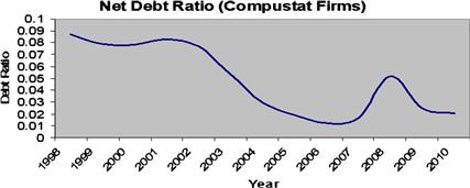
Figure 4 Net debt ratio for compustat firms (1998–2010). This figure shows the average net book debt ratio of Compustat Firms for each year from 1998 to 2010. Net book debt ratio is defined as (total long term liabilities + total current liabilities-cash)/(total assets).
Fosberg (2010) examines this issue by studying the effect of the large decrease in dividend tax rates (from as high as 38.6% to no higher than 15%) and moderate reduction in capital gains tax rates in 2003. Following such a large reduction in equity taxes, equity should become more attractive and debt less attractive. Fosberg documents a decrease in debt ratios following the tax cut, consistent with the theory of personal tax effects on capital structure. Surprisingly, the capital structure reductions are larger among firms that do not pay dividends, which seems counterintuitive. This only seems consistent with personal tax theory if equity tax rates are already capitalized into prices of non-paying firms, perhaps allowing the non-paying firms to have additional internal financial ability (relative to dividend payers) to decrease debt relative to equity. This seems like a fairly generous interpretation, however.
Graham (1999) tests similar predictions using firm-specific data. He finds that between 1989 and 1994 the net tax advantage of the first dollar of interest averaged between 140 and 650 basis points. 28 He finds that the firms for which the net advantage is the largest use the most debt in virtually every year. Graham also separately identifies a positive (negative) relation between the corporate tax rate (personal tax penalty) and debt usage. These results are consistent with Predictions 2 and 3.
Faccio and Xu (2011) examine debt usage in firms located in OECD countries. Section 2.3.1.2 summarized their finding that corporate income taxes and debt usage are positively related, though the results are not always statistically significant. They find much stronger evidence of the effects of personal tax influences on corporate debt usage. The authors report that higher tax rates on interest income lead to less corporate debt usage, and higher personal taxes on dividend income lead to more corporate debt usage. The estimated coefficients on these personal tax effects imply reactions that are three to four times larger than corporate tax influences. Faccio and Xu also find evidence of the personal tax effects hold in changes form, when interest or dividend tax rates change. Finally, they find that their results are stronger among the subset of firms that are most likely to make a capital structure change in the near future (i.e. firms far above or far below the country-year median).
Campello (2001) assumes that a given firm’s debt and equity are held by a particular clientele of investors (with the clienteles based on investor tax rates). He investigates the capital structure response to the large reduction in personal taxes (relative to the smaller reduction in corporate tax rates) after the Tax Reform Act of 1986. Campello finds that zero-dividend firms (which presumably have high-tax-rate investors and therefore experienced the largest reduction in the personal tax penalty) increased debt ratios in response to tax reform, while high-dividend payout firms (which presumably have low-tax-rate investors and therefore experienced a small reduction in the personal tax penalty) reduced debt usage relative to peer firms. Finally, Guenther (1992) investigates how corporations responded to the 1981 Economic Recovery Tax Act reduction in personal income tax rates, which increased the tax disadvantage for corporations. He finds that firms altered policies that contribute to the double taxation of equity payout: firms reduced dividends and instead returned capital by increasing the use of debt, share repurchases, and payments in mergers (which are often taxed as capital gains).
2.4.1 Market-Based Evidence on How Personal Taxes Affect Security Returns
The papers cited above, though consistent with personal taxes affecting corporate financing decisions in the manner suggested by Prediction 3, are not closely tied to market-based evidence about the tax characteristics of the marginal investor between debt and equity. Instead, these papers assume that dividend clienteles exist, and they also make assumptions about the personal tax characteristics of these clienteles based on a firm’s payout policy. For example, many of these papers implicitly assume that there is a certain marginal investor who owns both equity and debt and (to estimate τP) that this same investor sets prices between taxable and tax-free bonds. The truth is that we know very little about the identity or tax-status of the marginal investor(s) between any two sets of securities, and deducing this information is difficult.
For example, assume that munis yield 7%, Treasuries 10%, and equities 8% (and assume that this equity return has been adjusted to make it risk-equivalent to the risk of munis and Treasuries). In a Gordon/MacKie-Mason/Graham type of equilibrium, rmuni = rTreasury(1 − τP) = requity(1 − τequity) = 7%, which implies that τP = 30% and τequity = 12.5%. However, things are rarely so simple. First, it is difficult to determine the risk-adjusted equity return.29 Second, if there are frictions or transactions costs limiting arbitrage between pairs of markets (or if risk adjustments are not perfect), one could observe, say, munis yielding 7%, Treasuries 10%, and equities 12%. In this case, it is not clear which pair of securities should be used to deduce τP. If Treasuries and equities are used, the implicit τP could be negative. For example, assume that dividend payout is 15%, that τeffective cap gains = 5%, and that τequity is modeled as a weighted average between dividends and retained earnings: τequity = 0.15(1 − τdiv) + 0.85(1 − τeffective cap gains). To ensure that rTreasury(1 − τP) = requity(1 − τequity), in this example τP = −30% (assuming that τdiv = τP). Clearly, market frictions drive relative returns in this example, so the usual approach cannot be used to deduce the personal tax characteristics of the marginal investor(s).
Williams (2001) points out that when there are more than two assets, different pairs of assets can be arbitraged by different investors, so prices might reflect a mixture of tax characteristics. It is difficult to know which assets are directly benchmarked to each other by the marginal investor(s) and which are “indirectly arbitraged”, and it is even difficult to know whether capital gains or income tax rates are priced into security returns.
It would be helpful if future research could quantify the relative importance of personal taxes on security prices, with an eye toward feedback into capital structure decisions. One area in which a fair amount of research has been done along these lines involves determining the investor tax rate implicit between municipals and taxable government bonds. Poterba (1989) finds that the yield difference between high-grade one-year munis and government bonds approximates the top statutory personal tax rate, implying that the marginal investor between these two securities is a highly taxed individual. However, even this experiment is not without difficulty. First, returns on long-term munis and taxables imply a tax rate for the marginal investor that is approximately half that implied by the short-term securities. Chalmers (1998) shows that this holds even when the muni interest payments are prefunded by T-bonds held in defeasement (i.e. the muni interest is paid by earnings on a portfolio of government bonds purchased with the proceeds of the muni issuance), and therefore, risk differences between munis and T-bonds do not explain this conundrum. Green (1993) proposes that taxable bonds might not be “fully taxable” because a portion of their return can come from capital gains (especially for long-term bonds) and also because to some degree the interest income can be offset by investment interest deductions. Mankiw and Poterba (1996)suggest that munis might be benchmarked to equities by one clientele of investors and taxable bonds might be benchmarked to equities by another clientele. In this case, munis and taxables might not be directly benchmarked to each other, which could explain the unusual implicit tax rate that is sometimes observed between the two securities. Finally, recently Longstaff (2010) used an affine term-structure approach and estimated a high implicit marginal tax rate, putting us more or less back where we started.
As an example of trying to link the effects of personal taxes to capital structure issues, consider the implications from Engel et al. (1999) and Irvine and Rosenfeld (2000) about the personal tax penalty.30 Assume that corporations are the marginal investors in preferred stock but not in debt.31 Given the similarity of the securities, in equilibrium, we expect their after-investor-tax returns to be equal, within transactions cost bounds: rpreferred(1 − τDRD) = rMIPS(1 − τP). Plugging in rpreferred = 8.14% and rMIPS = 8.37% from Engel et al.’s Table 3, and assuming that the marginal corporate investor is taxed at 35% so that τDRD = 10.5%, we can back out the personal tax rate associated with interest income: 0.0814(1 − 0.105) = 0.0837(1 − τP) implies that τP = 13%. If we ignore the 30 basis point “yield premium” on MIPS imputed by Engel et al. and use rMIPS = 8.67%, τP = 16%.
Table 2 Tax incentive to use debt in a US multinational firm with foreign tax credits and allocable domestic interest. Assume that a US multinational firm currently returns $1 of pre-corporate-tax earnings to its marginal investor as domestic equity. The one-period model in this table shows the tax effect of instead paying the $1 as foreign interest (rightmost column in each panel) or as $1 of domestic interest (second-to-rightmost column). The model is adapted from Collins and Shackelford (1992) and assumes that all foreign income (IncFor) is repatriated every year and that tax rules are the same worldwide, except that only the United States allocates interest. The model ignores the AMT, carrybacks and carryforwards, personal taxes, and allocable items other than interest. Because the real-world tax-code is dynamic (i.e. it allows for carrybacks and carryforwards), the one-period nature of this model might overstate (understate) the largest (smallest) tax benefits. Note that foreign losses (i.e. IncFor − IntFor < 0) cannot be repatriated as losses back to the United States. FTCallow is allowable foreign tax credit (sometimes referred to as FTClimitation), FA is foreign assets net of foreign debt, WA is worldwide assets net of foreign debt, and FSI is foreign source income, which equals IncFor − IntFor − ![]() IntUS.
IntUS.

∗In a multiperiod model, FTCs above the allowable amount could be carried back or accumulated and carried forward. For example, in the excess credit case with interest allocation (row 5), ![]() of unused FTCs accumulate per incremental dollar of domestic interest.
of unused FTCs accumulate per incremental dollar of domestic interest.
Table 3 Summary of predictions and empirical evidence for multinational capital structure
| Prediction | Empirical evidence |
| Firm uses less debt when it has accumulated FTCs | None |
| Excess credit firms should have less incentive than deficit credit firms to use domestic debt. The incentive for excess credit firms to use domestic debt declines with the proportion of assets that are foreign. The incentive to use foreign debt increases in the foreign tax rate. | Debt usage declines when firm is excess credit. The reduction is increasing in the fraction of assets that are foreign (Froot and Hines, 1995). Likelihood of issuing domestic debt is highest when deficit credit and decreases as FTC limitations increase (Newberry, 1998; Newberry and Dhaliwal, 2001). Excess credit firms’ use of foreign debt increases in τFor and in the share of foreign assets (Altshuler and Mintz, 1995). Debt ratios of foreign affiliates increase in τFor (Desai, 1997; Altshuler and Grubert, 2003). |
| If domestic losses, use foreign debt. | US multinationals borrow in foreign subsidiary when they have domestic NOL carryforwards (Newberry and Dhaliwal, 2001). |
| Use a different financing source than domestic debt, especially when foreign assets are substantial. For example, use leases instead of debt because lease payments are not allocated to foreign operations. | Weak evidence that excess credit firms lease more than other firms (Froot and Hines, 1995). US firms’ incentive to finance with preferred stock rather than debt increases with proportion foreign assets (Collins and Shackelford, 1992; Newberry, 1998). |
| Use internal debt infusion rather than internal equity to finance foreign subsidiary, especially when τFor is high. Similarly, finance via royalty agreement rather than with equity. | Net internal borrowing by subsidiary from parent increases in τFor (Desai, 1997). Increase royalty payments when cheaper than repatriating dividends (Hines, 1995). |
| Use transfer pricing to increase (decrease) cash flow to low (high) tax affiliate. | Multinationals overinvoice low-tax affiliates (Lall, 1973).Foreign-controlled US firms’ US tax expense is inversely related to difference between the US and global tax rate (Mills and Newberry, 2000). |
| Repatriate dividends when excess credit. Repatriation for deficit credit firms negatively related to τUS -τFor.Remit dividends from high- and low-foreign-tax firms simultaneously, to reduce potential domestic taxes. | Excess credit firms repatriate more than deficit credit firms, and repatriation by deficit credit firms is inversely related to the cost of doing so (Hines and Hubbard, 1990).Most repatriated dividends are “cross-credited” (Altshuler and Newlon, 1993). |
| Borrow via US subsidiary that is lessthan 80% owned by multinational parent. | Example: Ford Motor Co. set up domestic financing subsidiary of which it owned 75% (Scholes et al., 2002). |
| Use triangle arrangements between subsidiaries in foreign jurisdictions with different tax burdens to reduce domestic taxes owed on remittances. | Low-foreign-tax subsidiaries invest in high-tax affiliate subsidiaries, which in turn remit funds to US parent at low or zero domestic tax liability; or low-foreign-tax subsidiaries are capitalized by high-tax affiliate subsidiary, so repatriations from high-tax subsidiary are assigned a foreign tax rate that is a mixture of the low- and high-tax rates (Altshuler and Grubert, 2003). |
To the extent that results based on MIPS interest carry over to debt interest, finding τP = 16% for the marginal debt investor is intriguing. First, note that the mean after-financing corporate tax rate in the 1993–1999 sample period is approximately 18% (see Table 1), which is a rough estimate of the tax benefit of the last dollar of interest deduction (ignoring all costs). If we make Miller’s (1977) assumptions that τE = 0 and that all firms face the same 18% marginal benefit of debt, then τP should equal 18% (i.e. MC should equal MB), quite close to the τP = 16% MIPS estimate. As argued by Green and Hollifield (2003), it would only take fairly small costs of bankruptcy to equalize the costs and benefits of debt, creating an environment conducive to equilibrium with internal optimal debt ratios. However, τE is most likely not zero for the marginal investor in equities. (Green and Hollifield argue that deferral reduces effective τE to about half its statutory level.) Another issue is that the estimated MIPS costs and benefits are average, not marginal. Even if the marginal costs and benefits are equal in an equilibrium like that depicted in Figure 2a, there is a firm surplus/benefit to using debt. Therefore, even if personal tax costs are large enough at the margin to equal marginal benefits, there appear to be tax-driven preferred capital structures for some firms. Presumably, the incremental tax savings would be near $0.35 per dollar for high-tax-rate firms, while the personal tax cost is only half that amount. Only if the nontax costs of debt are large for these high-tax-rate firms could a full Miller equilibrium hold, in which the benefits of debt are zero for all firms in equilibrium.
In sum, the implicit personal tax costs estimated here suggest that at the margin the tax costs and tax benefits might be of similar magnitude. However, they do not explain cross-sectionally why some inframarginal firms (with large tax benefits of interest) do not use more debt. (More details on this issue are presented in Section 2.4) One other area in which there has been a fair amount of success in deducing marginal investor tax characteristics—though not unambiguously so—is related to ex-day dividend returns. This discussion is deferred to Section 4, which explores how taxes affect corporate dividend policy.
In the most general sense, any research that shows that personal tax rates affect security returns sheds light on Miller’s (1977) claims. Using the CAPM-with-taxes specification, Auerbach (1983) finds evidence that tax-related preferences result in clienteles of investors that purchase stocks based on firm-specific dividend-price ratios. Constantinides (1983) and Dammon, Spatt, and Zhang (2001) investigate how favorable capital gains taxation affects investment and consumption choices. Seida and Wempe (2000) show that individual investors accelerated recognizing capital gains (and delayed losses) in anticipation of the increase in capital gains tax rates associated with the 1986 tax act. For a review of articles related to how personal taxation affects the timing and value of asset sales and purchases, see Poterba (2001).
2.4.1.1 Tax Capitalization
Another group of papers investigates tax capitalization and argues that personal taxes are capitalized into share prices via retained earnings. This in turn affects the relative tax advantage to debt because retained earnings are assumed to be the marginal source of funding. Harris and Kemsley (1999), Collins and Kemsley (2000), and related papers assume that all earnings are eventually paid out as taxable dividends (and none via repurchases or liquidating dividends), which is consistent with the “new view” of the effects of dividend taxation.32 They argue that (nearly) full dividend taxation is impounded into share prices and that, as a result, no incremental personal tax penalty is imposed when a firm pays a dividend.
Harris and Kemsley (1999) regress stock price on variables, including retained earnings, and they infer that retained earnings are penalized at a dividend tax rate of approximately 47%. Collins and Kemsley (2000) argue that reinvesting current earnings leads to investor capital gains taxation when shares are sold, on top of the already impounded dividend taxation. This logic implies that there is no personal tax penalty for dividend payments (it is already impounded into share prices, and therefore paying a dividend does not lead to further valuation effects). In fact, this leads to the counterintuitive argument that paying dividends leads to a reduction in future capital gains payments and therefore, dividend payments are tax advantageous. This implication only holds if arbitrage by tax-free investors is restricted to the point that personal investors are the marginal price-setters in stocks. Collins and Kemsley find empirical evidence that they interpret as being consistent with their hypotheses. An untested implication of their argument is that there should be a large value gain in deals that result in firms returning capital to investors in any form other than taxable dividends (such as mergers). Research into this area could be informative.
Rather than dividend taxes, an alternative argument is that capital gains taxes on future earnings are impounded into share prices. Consider a shareholder in a nondividend-paying firm and assume that the firm is expected to pay dividends at some point in the distant future. If the market expects that low-tax investors are likely to be the dominant owners of this company when the dividend payments are initiated, the only (future) tax that current investors face is capital gains. In support of this argument, Lang and Shackelford (2000) show that upon announcement that capital gains tax rates were going to decline, stock prices increased most among firms for which capital gains are most important (i.e. firms with the lowest dividend yield). In lock-in models such as Klein (2001), for firms with substantial accrued retained earnings, returns fall when capital gains rates fall because the required return declines along with the tax rate. For further discussion of the tax capitalization literature, see Shackelford and Shevlin (2001). Dai et al. (2008) also show that the equilibrium impact of capital gains taxes reflects both capitalization as well as the lock-in effect where capital gains taxes decrease supply.
Overall, the tax status of the marginal investor, and therefore the empirical magnitude of the personal tax penalty, is an open empirical question. This is an important issue. For one thing, failing to control for personal tax considerations can result in an omitted variable bias. For example, personal tax considerations could cause clientele behavior that is correlated with dividend-payout ratios. In a regression that omits personal tax considerations, the dividend-payout coefficient might erroneously be interpreted as supporting a nontax hypothesis. As another example, business students are often taught that the tax advantage of debt is captured by τCD (see Eqn (4)), which ignores personal tax effects. If it can be demonstrated that personal tax effects are not particularly important, this simplified view of the world might be justified. In contrast, if investor taxes affect security returns in important ways, more care needs to be taken in modeling these effects in corporate finance research. Investigations of personal tax effects face several challenges, not the least of which is that risk differences between securities must be properly controlled to allow one to deduce implicit tax rates from market return data. Another risk is the great difficulty in estimating personal tax effects with any precision.
2.5 Beyond Debt vs. Equity
2.5.1 Leasing
The discussion thus far has considered the debt versus equity choice; however, it can be extended to leasing. In certain circumstances, a high-tax-rate firm can have a tax incentive to borrow to purchase an asset, even if it allows another firm to lease and use the asset. With true leases (as defined by the IRS), the lessor purchases an asset and deducts depreciation and (if it borrows to buy) interest from taxable income. The lessee, in turn, obtains use of the asset but cannot deduct interest or depreciation. The depreciation effect therefore encourages low-tax-rate firms to lease assets from high-tax-rate lessors. This occurs because the lessee effectively “sells” the depreciation (and associated tax deduction) to the lessor, who values it more highly (assuming that the lessee has a lower tax rate than the lessor). This incentive for low-tax-rate firms to lease is magnified when depreciation is accelerated, relative to straight-line depreciation. Furthermore, the alternative minimum tax (AMT) system can provide an additional incentive for a lessee to lease, in order to remove some depreciation from its books in an attempt to stay out of AMT status.
There are other tax effects that can reinforce or offset the incentive for low-tax-rate firms to lease. Lessors with relatively large tax rates receive a relatively large tax benefit of debt, which provides an additional incentive (to borrow to) buy an asset and lease it to the lessee. Moreover, tax incentives provided by investment tax credits (which have existed at various times) associated with asset purchases are also relatively beneficial to high-tax-rate lessors. In contrast, the relatively high taxes that the lessor must pay on lease income provide a tax disincentive for firms with high tax rates to be lessors (and similarly the relatively small tax benefit that a low-tax-rate firm obtains from deducting lease expense works against the incentive for low-tax-rate firms to lease rather than buy). The traditional argument is that low-tax-rate firms have a tax incentive to lease from high-tax-rate lessors, though this implication is only true for some combinations of tax rules (e.g. depreciation rules, range of corporate tax rates, existence of investment tax credits, or AMT) and leasing arrangements (e.g. structure of lease payments). See Smith and Wakeman (1985) and Eisfeldt and Rampini (2009) for details on how nontax effects can also influence the leasing decision.
Prediction 5: All else equal, the traditional argument is that low-tax-rate firms should lease assets from high-tax-rate lessors, though this implication is conditional on specifics of the tax code and leasing contract.
There are several complications associated with investigating whether firms lease in response to tax incentives. First, because leasing expense is tax deductible, leasing endogenously reduces a lessee’s effective tax rate, which can bias an experiment in favor of detecting tax effects. Similarly, lessor tax rates could be endogenously increased from the effects of lease income. Second, financial statement definitions of leasing are not one-to-one with IRS definitions, making it difficult to use Compustat data to test Prediction 5.33 Using endogenously affected tax variables, Barclay et al. (1995b) and Sharpe and Nguyen (1995) find that low-tax-rate firms use relatively many capital leases. However, capital leases do not meet the IRS definition of true leases. (Instead, they are likely a mixture of true leases and conditional sales contracts, the latter of which are treated like debt, so that the lessee deducts interest and depreciation, and one might expect to find a positive relation between the conditional sales contract in capital leasing and taxes.) Therefore, the documented negative relation between capital leases and taxes is hard to interpret because it might be spurious.
Graham et al. (1998) address the first issue (endogeneity) by measuring tax incentives “but-for financing decisions”, that is, calculating tax rates using income before debt interest and the implicit interest portion of lease payments are deducted. They address the second issue by focusing on operating leases, which are defined in a manner similar to the IRS definition of true leases. Graham et al. (1998) find that the use of operating leases is negatively related to before-financing tax rates, consistent with Prediction 5, and that capital leases are unrelated to before-financing tax rates. Graham et al. also show that erroneously using an after-financing tax rate would double the magnitude of the negative tax coefficient for operating leases, and spuriously assign a negative tax coefficient to capital lease usage.
Eades and Marston (2001) find that lessors tend to be high-tax-rate firms (consistent with Prediction 5). Finally, O’Malley (1996) finds no evidence that firms systematically lease in response to tax incentives imposed by the AMT. We need research investigating whether the tax benefit of leasing adds to firm value. The jury is still out on whether debt and leasing are substitutes for the lessee (as they might be in the sense considered by DeAngelo and Masulis (1980), because both lead to tax deductions).
2.5.2 Pensions
Black (1980) argues that pension plans and the overall company are a single economic entity that should have an integrated financing and investment strategy. Due to interest tax deductions, the cost of corporate borrowing is the after-tax cost of debt. Because they are tax-free entities, defined benefit pension plans (DBs) earn the before-tax rate of interest on bondholdings. Therefore, Black suggests that DBs should increase (decrease) bond (equity) holdings, while the rest of the firm should do the reverse. This action should not increase firm risk because the increase in corporate debt offerings is offset by the increase in bonds held in the pension plan. (Interestingly, though, Shivdasani and Stefanascu (2010) find that US debt ratios are 35% larger when pension assets and liabilities are incorporated into measures of capital structure.) In an MM (1963) world, the net effect is that the company earns τC times the amount of bonds held, as in Eqn (4). Tepper (1981) argues that there can be a tax advantage to the strategy of corporate borrowing and DBs investing in bonds, even in a Miller (1977) world. In this case, the benefit occurs when the DB is an inframarginal investor in bonds, thereby earning the “extra” return necessary to compensate individual investors for the personal tax penalty associated with interest income (i.e. DBs capture some of the investor surplus depicted in Figure 2). The Tepper incentive for DBs to hold bonds increases with the difference between personal tax rates on interest and equity income.
Prediction 6: Defined benefit pension plans have an incentive to hold bonds (equity) that increases (decreases) in the corporate tax rate, while the rest of the firm has the reverse incentive.
Myers (2001) finds evidence consistent with the Black (1980) case: she reports that DB bondholdings increase with a simulated corporate marginal tax rate. She does not find evidence consistent with the Tepper argument. In a less direct test of the same incentives because it focuses on the size of pension contributions rather than pension capital structure, Thomas (1988) finds time-series evidence that firms decrease DB contributions when their tax rate is falling, and cross-sectional evidence that high-tax firms have larger DB funding levels.
Clinch and Shibano (1996) study pension reversions, which occur when a firm terminates an overfunded pension, settles its liabilities, and reverts the excess assets to the firm, all in one year. The reverted assets are taxable in the reversion year. Clinch and Shibano state that firms with the largest tax benefit of reverting do so, and also that firms’ time-reversion decisions occur in years with particularly large tax benefits. One nice aspect of the Clinch and Shibano experiment is that their tax variable equals the tax consequence of reverting relative to the tax consequence associated with the next best alternative (e.g. amortizing the excess assets over several years) rather than a “do nothing” alternative.34
2.5.3 Debt Maturity
In the spirit of Modigliani and Miller (1958), Lewis (1990) derives an irrelevance null hypothesis for debt maturity. If corporate taxes are the only market imperfection, Lewis shows that the optimal firm-specific debt policy (i.e. optimal level of promised interest payments) can be achieved by various combinations of short- and long-term debt. This implies that firm value is unaffected by debt maturity structure and that capital market imperfections beyond corporate taxes, like costs to restructuring debt or underinvestment, are needed for debt maturity to matter. (Incomplete contracts can also lead to debt maturity mattering.)
Rather than modeling the simultaneous choice of debt level and maturity structure as in Lewis (1990), Brick and Ravid (1985) assume that firms choose debt level before debt maturity. If the expectations theory of interest rates holds, firms pay the same present value of interest in the long run regardless of debt maturity. However, issuing long-term debt accelerates interest payments, thus maximizing the present value of the interest tax shield. Brick and Ravid (1985) use this logic to argue that debt maturity should increase with the slope in the yield curve.
Prediction 7: Debt maturity increases in the slope in the yield curve.
Most empirical evidence does not support this prediction. Barclay and Smith (1995a) and Stohs and Mauer (1996) include a stand-alone yield curve variable that is either insignificant or has the wrong sign. Guedes and Opler (1996) maintain that the slope of the yield curve should only affect firms with a positive tax rate, and therefore the yield curve variable should interact with the corporate marginal tax rate. Neither Guedes and Opler (using a crude measure of the corporate tax rate) nor Harwood and Manzon (1998) (using a simulated corporate tax rate) find a significant coefficient on the yield curve variable. The one exception is Newberry and Novack (1999), who use a dummy variable equal to one during 1992 and 1993 (when the term premium was relatively high) and equal to zero for all other years 1987–1995. Newberry and Novack find a positive coefficient on the yield curve dummy in their public debt regression but not in their private debt analysis.
Kane, Marcus, and McDonald (1985) determine optimal debt maturity in a model that trades off corporate tax benefits with personal tax, bankruptcy, and flotation costs. The implications of their model are that debt maturity decreases with the corporate MTR and increases with the personal tax rate: long maturity implies less frequent recapitalization and relatively low transactions costs, so long-term debt can be desirable even if the net tax benefit is low. Maturity also decreases with the volatility of firm value because volatile firms are more likely to restructure debt.
Prediction 8: Debt maturity decreases with the corporate MTR and the volatility of firm value and increases with the personal tax rate.
Stohs and Mauer (1996) find the following support for Prediction 8: volatile firms generally use shorter term debt. The evidence relating to the tax-rate prediction is weaker. Stohs and Mauer report that debt maturity decreases with corporate tax rates—but their MTR variable is very crude (equal to income tax expense divided by pretax income when this ratio is between 0 and 1, and equal to 0 otherwise). Opler and Guedes (1996) find a negative coefficient on a tax expense divided by assets variable but the wrong sign on an NOL-based tax variable. Finally, Harwood and Manzon (1998) and Newberry and Novack (1999) point to a positive relation between a simulated tax rate variable and debt maturity, opposite the Kane et al. prediction.35 A positive coefficient makes sense if large simulated MTRs identify firms that use long-term debt because they are relatively likely to be able to deduct interest in current and future periods.
Finally, debt maturity can affect the tax-timing option for firms to opportunely retire debt (e.g. Emery, Lewellen, and Mauer, 1988). If the corporate tax function is convex, the expected present value tax benefit of short-term debt declines with interest rate volatility, while the tax deductions with long-term debt are fixed. Therefore, long-term debt is preferred when interest rates are volatile. Long-term debt also increases the value of the timing option for investors to tax-trade securities (Kim, Maurer, and Stohs, 1995) because option value increases with security maturity and long-term bond prices are more sensitive to changes in interest rates.
Prediction 9: Debt maturity increases with interest rate volatility.
Kim et al. (1995) find that debt maturity increases with interest rate volatility, but Guedes and Opler (1996) do not. Nor do Guedes and Opler find significance for a second variable that interacts interest rate volatility with a corporate MTR variable.
In an analysis conducted for this chapter, I perform a more direct test on the hypothesis that uncertainty about future tax-paying status reduces the use of long-term debt. I use the standard deviation of the simulated marginal tax rate to measure uncertainty about tax-paying status, with the standard deviation calculated across the simulated scenarios for any given firm-year. I do not find any relation between debt maturity and uncertainty about tax-paying status.
The evidence linking tax incentives to debt maturity is mixed. One factor that makes it difficult to draw general conclusions is that debt maturity is defined differently in various papers. Barclay et al. (1995a) use a dependent variable measuring the portion of outstanding debt that matures in four or more years; Guedes and Opler (1996) use the log of the term to maturity for new debt issues; Stohs and Mauer (1996) use the book value weighted average of the maturity of a firm’s outstanding debt; Newberry and Novack (1999) use the same for new issues; and Harwood and Manzon (1998) use the portion of outstanding debt that is long term. Another issue that might affect inferences about tax variables is the apparently nonlinear relation between debt maturity and nontax influences (Guedes and Opler, 1996). Unless the nonlinearity of the overall specification is properly controlled, it might adversely affect the ability to detect tax effects. Finally, the yield curve was never inverted during the periods studied by most of these papers, so the tests of Brick and Ravid (1985) focus on the steepness of the yield curve rather than on the sign.