2.1 Framework for modeling risk

The objectives of both models reflect a tradeoff between expected return and some measure of risk. As a portfolio manager who’s performance is measured relative to a benchmark, the risk is to under-perform the benchmark. As financial director responsible for the financial health of a life insurance company, the risks typically involve falling below thresholds for capital adequacy, solvency, or other legal requirements or to achieve lower returns on assets relative to competitors.

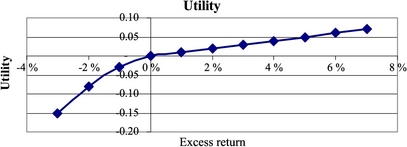
In order to use a quantitative approach to the asset allocation problem the various risks must be quantified. To do this, we introduce targets from which shortfalls will be associated with a cost (in excess of the actual cost in terms of reduced value of the assets). These targets can be an absolute return target (for instance, 0% return), relative return targets (the return on some benchmark) or financial targets like capital adequacy and solvency requirements. A shortfall cost function measures the (subjective) cost of shortfalls of different magnitudes. We assume a convex shortfall cost function, i.e., increasing marginal penalty. A simple quadratic version of such a shortfall cost function is illustrated in Figure 1.

Fig. 1 A shortfall cost function with quadratic penalty.

The objective of the optimization is to maximize the expected return net of expected shortfall costs. The objective function will be linear for returns above the target return and strictly concave for returns below the target return. The utility function consistent with the shortfall cost function in Figure 1 is shown in Figure 2. For a comprehensive discussion of risk and utility functions, see Bell (1995).

Fig. 2 The utility function consistent with the shortfall cost function in Figure 1.

To identify risk preferences there are at least two major approaches. One is to define risk based on theoretical considerations, studying the theory of market risk and individual risk attitudes. The other is to focus on how the user sees his own risks, and model accordingly. The approach using shortfall cost functions as described, is an example of the latter way of thinking. The choice of which risks to include and what parameters to use, is done in close cooperation with the user. It is useful to observe that the result can be interpreted as a utility function, but our goal has not been to produce a utility function.

A utility function, like the one in Figure 2, has several parameters describing its shape. In our case, these parameters were defined in close interaction with the user. Initially, we ran the model with one set, discussed the model results with the user, and the user concluded such as “We are not that risk averse”, or “This is too risky relative to so-and-so legal constraint”. Eventually, a utility function reflecting the user’s view on his own risks is derived. We believe that this is the most reasonable way of setting up an objective function reflecting risk. For a discussion, see Kallberg and Ziemba (1983).

Of course, there are many other risks involved, the major one being whether or not a model makes sense in the first place. When discussing the track record of the model in Section 5, we shall return to this issue. A variety of tests can be done, but they will all depend on certain assumptions, and there will always be an aspect of belief or hope in the decision to use a model.

2.2 Risk measures

At the strategic level, the risks can be split into balance risk and competitor risk. The asset liability management is influenced by the following legal framework issues:

The capital adequacy requirement states that the buffer capital (mainly equity and subordinated debt) must exceed 8% of the value of risk-adjusted assets. The assets are assigned risk weights, with for instance equity counting 100% and Norwegian money market investments counting 0%. If, for example, all assets were invested in equities, then the buffer capital of the company had to be 8% of the total balance. The solvency requirement states that the buffer capital of the company must be larger than a percentage of the pension liabilities. Both requirements need to be modeled because both can be binding dependent on the asset mix.

The minimum guaranteed return is currently about 3.8% per annum as an average for existing customers. The guarantee applies for every single year. If the return on assets is lower than the guaranteed return, buffer capital must be used in order to fulfill the guarantee. If the company achieves a profit after costs, and after the guaranteed rate of return is paid, the regulations state that a minimum of 70% must be returned to the customers. These two regulations have severe impact on the long-term planning of the insurance company. If return on assets is well below the guarantee in a given year, the buffer capital must be used to cover the guarantee, and rebuilding the buffer capital is a slow process since a maximum of 30% of a year’s profit (after costs and guaranteed rate of return) can be used for this purpose. As a result one bad year can have severe long-term effects on the risk capacity and hence on future returns.

The customers’ right to move their policies, free of charge, creates a very competitive environment and makes it crucial not to under-perform the competitors in any year. The goal of not under-performing the competitors will in some situations conflict with the goal of securing the long-term financial health of the company.

The strategic ALM model incorporates three shortfall variables: Capital adequacy, solvency requirement and return relative to the competitors. Setting targets from which to measure the shortfalls and estimating the cost function are challenging tasks. Targets are typically set higher than the legal minimums, and the marginal costs are increasing. At the point where the company is close to bankruptcy, the marginal costs clearly increase dramatically.

The shortfall costs are difficult to estimate accurately, but they are “real” costs in the sense that they should reflect the business costs of under-performing the targets. It is straightforward to estimate their limit values; they will vary between zero and the value of the company. The shortfall cost functions can be estimated. The cost of under-performing the competitors, for example, can be estimated by finding the average cost of losing one customer, and estimating the relationship between under-performing the competitors and the expected number of customers lost. In the multi-period setting, we have added shortfall costs over periods. From a theoretical point of view, additivity in utility is a very strong assumption. However, the user is satisfied with the implications of such an assumption, particularly taking into account that the decision-maker is a company and not an individual.

The legal regulations and their effect on the decision-making in a life insurance company is elaborated, and a mathematical description of the model given, in Høyland and Wallace (2001b). Similar studies have been undertaken for a casualty insurance company in Gaivoronski and De Lange (2000). de Lange, Fleten and Gaivoronski (2004) and Gaivoronski, Høyland and De Lange (2000) also address ALM-planning in the casualty insurance business.

For the TAA-problem, the legal framework is, to a large extent, defined by the mandate given by the client. For the funds that the TAA-group manages for the life insurance company, the mandate is usually given by a benchmark, risk limits relative to the benchmark, and constraints defining upper and lower limits for each asset class. The task of the TAA-team is to achieve excess return relative to the benchmark, while operating within its risk limits and constraints. As a manager evaluated on a relative basis, the risk is to under-perform the benchmark. The shortfall costs in this case should reflect the expected future loss by potentially losing the client in case of a shortfall, and also the subjective personal utility functions of the portfolio managers. Note that there are less conflicting goals with different time horizons in this problem, and hence the need for a multi-period setting is less than for the strategic problem, see more on this in Section 2.5.

2.3 Investment vehicles

For the strategic ALM problem, the model is typically applied for the planning of the following financial year, and two problems are solved simultaneously: The allocation between major asset classes and the structure of the liability side of the balance sheet. The investment universe is split into a limited number of broad asset classes: typically, domestic and international stocks, domestic and international bonds, domestic money market, and real estate. The task of the SAA-team is to establish a benchmark allocation between these asset classes. Most of the currency risk is hedged. By law, the maximum currency exposure is 15% of the liabilities.

For the TAA-problem, active market positions are implemented via derivatives. The TAA-model applies for both linear, e.g., futures and non-linear, e.g., options, derivatives. The asset classes defined within the investment universe are money market, bonds, equities, currencies, and commodities. USA, Japan, UK, EMU-area, Norway, and Sweden are potential regions for investments.

For the money market, the investment vehicles are futures on the LIBOR interest rates at different expiry dates. For bonds, they are two-, five-, and ten-year bonds. For equities, the investment vehicles are the most liquid futures in each region. For currencies, the number of potential asset classes equals the number of regions less one, since we define all currencies relative to the US dollar. All together, the investment universe consists of more than 40 assets. The number of assets included in each run will, however, be much smaller, typically 15–25. One part of the investment process is to select the asset classes on which we have the strongest views.

Note that the currency risk is small when dealing with derivatives. Only the margin accounts in foreign currency (which for equities are less than 10% of the exposure, and for bonds even less) are exposed to currency risk. In the TAA-problem currencies are treated as any other asset class. Currency exposure is only accepted if it is the result of an active view on the return from investing in a currency cross. With no active view on currencies, significant currency exposures will be hedged. As the performance of the fund is measured in Norwegian kroner (NOK), NOK is the base currency.

There are several reasons for using derivatives instead of cash instruments:

Most of the standardized derivatives used are highly liquid, often more liquid than the underlying cash instrument. The transaction costs are lower due to lower execution fees and less market impact. Further, a derivatives strategy can be put on top of any underlying cash portfolio. This means that a strategy can be implemented efficiently across different clients with different underlying portfolios. Finally, the use of options allows for a much larger degree of tailor-made portfolios relative to the portfolio managers’ view on the market.

The modeling implications of using derivatives are minor. The market expectations are given on the underlying assets and it is usually straightforward to calculate the future value of the derivatives given the future value of the underlying.

2.4 Constraints

Both models have both soft and hard constraints. The soft constraints are defined by the shortfall variables, and the shape of the shortfall cost function defines the softness.

The SAA-model has the following constraints:

Høyland and Wallace (2001b) describe the legal framework in more detail.

The TAA-model has three types of constraints:

For both models, all constraints are linear. A mathematical description of a simple version of the model is given in the equation below. To simplify the presentation we have presented a single period TAA-model that assumes cash investing, where short selling is allowed, and we have left options out. We have assumed a target return of zero.

Define the following parameters:

	probability of scenario s,
	return on asset i in scenario s,
A,B	shortfall cost parameters,
	lower and upper liquidity bound,
	lower and upper subjective bound,

and the variables

	investment in asset i,
	shortfall in scenario s.

The mathematical model is then:

A linear plus quadratic shortfall cost function is chosen. The linear term is included in order not to underestimate the penalty cost for small shortfalls. An iterative procedure is applied where α is tuned until the target risk level is achieved.

2.5 The single versus multi-period framework

In the literature many papers argue for dynamic, multi-period models, see, for example, Cariño and Ziemba (1998), Consigli and Dempster (1998), and Consiglio, Cocco and Zenios (2001); Kouwenberg and Zenios (2006) and Dert (1995). We agree with the arguments given by these authors, but we argue that the value of a multi-period framework depends on the problem to be solved, and that there might also exist good reasons for choosing a single period framework.

In Section 2.2 risk measures for our two models were discussed and for the SAA-problem we concluded there were more conflicting goals with different time horizon than in the TAA-model. For the SAA-model, it would be impossible to model these conflicting goals in a single period framework, whereas for the TAA-problem, the risks are realistically described in a single period model.

Furthermore, there are more pragmatic issues to be considered when deciding upon the dynamics of a model. One needs to consider the frequency of model runs, and the construction of input data. For the TAA-problem, the estimations of the input data are extensive and time consuming, and the model is run on a monthly or more frequent basis. A multi-period framework radically increases the number of input parameters that must be estimated or specified, so moving to a multi-period setting would be a severe challenge from a practical point of view. Clearly, if the necessary distributions are too extensive, the quality of the input data will decrease. See Section 3 for a discussion on generating the input data, and see the case study in Section 5 for a detailed description of how the input data is specified for the TAA-model.

The SAA-problem is solved for fewer asset classes and it is also solved less frequently. For the SAA-model, a multi-period framework is chosen; the model currently in use has two periods (technically a three-stage stochastic programming model). Despite the potential advantages of a multi-period framework, the TAA-team uses a single period model (two-stages) for the tactical model.

In the future we will consider moving into a multi-period framework also for the tactical model, and investigate further the advantages and disadvantages. In particular, we believe that the multi-period setting is useful when options are allowed as investment vehicles. In addition we hope to achieve a better understanding of the dynamics of portfolio management by analyzing the solutions from a multi-period decision model. The challenge will be to secure high quality input data, in particular, the inter-period dependencies of the uncertain variables need to be investigated.

2.6 Comparison with the mean-variance model

The standard mean-variance model has a single period whereas the SAA-model has multiple periods. See the previous section for a discussion of advantages and disadvantages regarding the choice of a static versus a dynamic model. In addition, our models differ from the standard mean-variance framework in at least four aspects:

We saw in Section 2.3 that derivatives are used as investment vehicles for the TAA-model. When trading futures, the transaction costs in terms of broker fees are relatively low. The transaction costs are, however, larger if we take into account the bid offer spread cost and the potential market impact cost. With cash instruments as investment vehicles the total transaction costs are usually larger. With all costs included, the transaction costs influence the optimal asset allocation mix. While in the standard mean-variance model, transaction costs are not taken into account, both the TAA- and the SAA-model incorporate transaction costs.

Section 2.2 described how risk is defined in both models. Only downside risk is penalized in the objective function. This is in contrast to the mean-variance framework, where deviations from the mean, both down- and upward, are treated equally. With symmetric return distributions (as the mean-variance framework assumes) this is only a conceptual problem, since using semi- (downside) variance or variance as risk measures will lead to the same solution. However, with asymmetrical distributions this is not the case. We allow for asymmetrical distributions in both the TAA- and SAA-model.

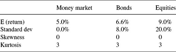
Let us illustrate and quantify the effect of asymmetrical distributions with an example. Consider a case with three asset classes; cash, bonds and equities. Expectations for the returns on these asset classes are given in Tables 1 and 2. Note that the expectations in Tables 1 and 2 are consistent with a multi-variate normal distribution. We now run the scenario generation model and create 1000 outcomes with statistical properties as in Tables 1 and 2. We then solve with the mean-variance model and the model proposed in this paper, while targeting equal risk levels (in terms of the variance of the return of the portfolio). With a reasonable shortfall cost function, the optimal solutions obtained from the two approaches are equal for all practical purposes. Now, let us assume that the return distribution for equities is skewed to the right as in Figure 3. Solving the mean-variance model leads to exactly the same solution as before, since this model only reacts to the two first moments of the distribution. With the asymmetrical risk measure however, the optimal holding of equities rises from 17.5 to 26.4%. (In addition to the market expectations, the only other inputs are the parameters defining the shape of the shortfall cost functions. Changing these parameters within reasonable bounds does not significantly alter the results.)

Table 1 Marginal central moments

Table 2 Correlation estimates

Fig. 3 A distribution with skewness of +1.

The equity holding increased because the (positive) asymmetry in the return distribution of equities fits the asymmetry of the utility function. As explained in Section 2.1, the objective is to maximize the expected return net of expected shortfall costs, where the marginal shortfall cost is increasing with respect to the shortfall. Since outcomes with relatively large negative excess returns give large negative contributions to the objective function value, the model will seek to avoid such outcomes. Since a right skewed return distribution has less probability mass in the left tail of the distribution relative to a symmetrical return distribution, the right skewed return distribution will be preferred relative to a symmetric return distribution (all other factors being equal).

The above example leads us to the final difference between the two approaches. The mean-variance model has been criticized for being over-sensitive to changes to the input parameters, in particular to the expected returns. Chopra and Ziemba (1993) find in their investigations that the relative importance between means, variances and covariances is about 20:2:1, but such that the importance of the mean can be even higher depending on the level of risk aversion. With our framework, the sensitivity is lower. This is because there are other properties than the mean, variance and the correlations that stabilize the optimal solution with respect to changes in these properties. As argued above, the model will for example prefer asset classes that are positively skewed as they fit the utility function. At this point however, this is only an empirical and intuitive result, which can be of interest for future research. See also Dupacova (2001) for a discussion on sensitivity analysis of financial models.

2.7 The linkage between the SAA-problem and the TAA-problem

In Section 2.5, the conflicting goals of the ALM-problem were described. The key is to find an asset allocation mix that takes into account the balance sheet risk, the competitor risk and the SAA-team’s longer term market expectations. Such an asset allocation is found with the help of the SAA-model and the cash is allocated to various asset managers who manage funds within each asset class. These mandates can be quite broad (for example, foreign equities) or they can be more specialized (for example, European Telecom). For each of these mandates a benchmark and risk limits relative to the benchmark are established. On top of the cash allocations within each asset class, the SAA group allocates risk to TAA-mandates, see Figure 4. This process of allocation risk at different levels and to different decision makers is in the literature called risk budgeting, see, for example, Rahl (2000) and the references therein for a discussion.

Fig. 4 Risk budgeting.

For the TAA mandate described in this paper the SAA group has allocated a limited amount of cash that is necessary to cover margin requirements on the TAA derivative positions. With little capital used the cost of capital in terms of alternative return is close to zero. Therefore, the benchmark return for the TAA-mandate has been set to zero.² The only constraint in the TAA-mandate is a risk constraint given by a Value at Risk limit, which is equivalent to a tracking error limit relative to a benchmark position vector that consist of zero’s.

3.1 Data collection

At a relatively low cost, almost unlimited amounts of data can be collected, whether empirical price data, macro economic data, micro economic data, or analyses from central banks and organizations like IMF and OECD. The data required to support a given decision model depends on the philosophy behind the modeling. The input to the decision models that have been reported in the stochastic programming literature, typically only requires empirical price data (and sometimes also empirical macro economic data). We will explain in the next section how the asset managers of Gjensidige-NOR use subjective judgments when estimating the input data of the decision models. To support that judgment, the key is to extract and structure the data that is relevant. It is however, out of the scope of this paper to explain this process in detail.

3.2 Formation of market expectations

In order to run a portfolio optimization model, one must elicit and quantify the market expectations. The number of asset classes in the TAA-model is typically between 15 and 25. It is a comprehensive task to specify, say, a 20-dimensional joint distribution. Several methodologies have been developed over the last few years. Many rely on regression procedures to reduce the number of random variables that needs to be identified and analyzed explicitly. This modeling is based on sampling or the development of stochastic processes (see, for example, Mulvey, 1996). The choice will depend on analytical preferences as well as the availability of data and understanding of the stochastic processes.

The asset managers of Gjensidige-NOR prefer to express market views by quantifying their return expectations for the asset classes directly. They preferred to describe the return of an asset class by its marginal distribution, and its interrelation with the other asset classes. This raises the question of which properties of a distribution are in fact important to capture correctly in order to have a good decision support model. Høyland and Wallace (2001a) discuss why the selection of important statistical properties is problem dependent. The Markowitz mean-variance model, for example, reacts to only the first two moments of a distribution (including the cross moments). Any efforts to obtain correct descriptions of higher moments are a waste of time since the model does not react to them.

To find a portfolio that has the best risk reward balance, it is necessary to estimate the expected portfolio return and some measure of uncertainty. Hence, expected value and standard deviation are obvious statistical properties that need to be specified. However, as we saw in Section 2.6, the shape of the probability distribution can influence the optimal portfolio choice to a large degree.³ Skewness and kurtosis give us the ability to express our subjective views on how the uncertainty is distributed around the mean for a given asset. The motivation for introducing the skewness and the kurtosis comes from two basic facts: Firstly, asset class returns are not normal, at least not with reasonably short time horizons, see, for example, Jackwerth and Rubinstein (1996), and secondly, the optimal portfolio is highly influenced by these distribution properties (for all reasonable utility functions).

For the asset allocation problems at hand, we concluded that for the marginal distributions, the first four moments (i.e., expected value, standard deviation, skewness and kurtosis) are needed to create a stable decision support model (see the next section for a discussion). For describing the relationship among asset classes, correlations were found to be enough. The first four moments of a marginal distribution can either be derived from the marginal return distributions, or they can be specified explicitly. As the experience of the asset managers has increased, the latter approach has become standard. Hence, describing market expectations is equivalent to describing the necessary moments and correlations.

It is a well-known fact that in stressed market conditions the longer-term average correlation structures tend to break down. This was the main reason for the failure of Long Term Capital Management, see Jorion (2000). Crash scenarios influence the optimal portfolio structure, and to capture the crash scenarios in an appropriate way, we split the future into two states, one “normal” state and one “crash” state, and then specify the marginal distributions and correlations separately for the two states. The two are then combined using an estimated probability of the two states occurring. This idea is later followed up by others. Geyer et al. (2002) use three sets of covariance matrices: 70% regular, 20% volatile, 10% crash. In crash, bonds and stocks are negatively correlated while in the other two they are positively correlated.

The portfolio managers find the possibility of expressing views on the asymmetry and the degree of fat tails on the return distributions very useful. In many cases, return distributions are obviously asymmetric. The zero level in interest rates, for instance, naturally creates asymmetry. There is less obvious asymmetry for equities, but the pricing of the market, relative to future expected earnings and the macro economic environment, often indicate whether potential large, longer-term moves are to the upside or to the downside.

Investors are always faced with the possibility of a stock market crash. The ability to express crash scenarios, and assign them probabilities, is considered to substantially increase the quality of the input data. Both the expected magnitude of a potential crash, and the probability for it to happen, are changing over time and the portfolio managers seek to have an active view on these factors.

3.3 Scenario generation

From a methodological point of view, there is no difference between how we generate scenarios for the two models. In this section we will explain our approach with reference to the single period tactical model. In Section 3.4, we will comment on the multi-period case.

Before turning to the technicalities of the scenario tree generation, let us explain our main philosophy. There is no general agreement among either scientists or practitioners about best practice. First, there is the issue of understanding the random variables. For most, the obvious staring point is data. However, from there we can go in many different directions. Some believe in estimating stochastic processes from the data. Others, and we belong to that group, prefer to add subjective information to the data. One issue is whether or not the past describes the future well. The decision-makers in Gjensidige Nor are not willing to invest on that assumption. Further, theory tells us how to extract implicit information from market data. Jackwerth and Rubinstein (1996) show how to derive the risk neutral return distributions from option prices. For a general overview over scenario generation methods, see Dupacova, Consigli and Wallace (2000).

At some point, the user will be satisfied with his description of the possible futures. He may have empirical data that he believes describes the future well, he may have some stochastic processes (estimated or guessed), he may have the possible futures extracted from market data, or he may simply have subjective views. But it is unlikely that the data is in a form suitable for stochastic programming. We think it is important to point out that the problem of making a scenario tree from specifications, whatever they are and wherever they come from, is a separate issue from understanding the random variables.

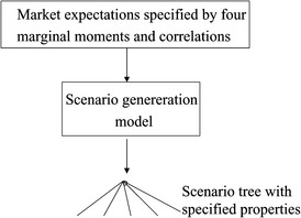
Our methodology is based on constructing a scenario tree from the specifications. We create the outcomes of the tree by using an iterative procedure that combines simulation, Cholesky decomposition and various transformations, see Høyland, Kaut and Wallace (2003) for details. The scenario generation process is illustrated in Figure 5: The scenario generation model constructs a limited set of outcomes, in the academic literature known as a scenario tree, which is consistent with the specified moments and correlations, i.e., the tree has exactly the required properties.

Fig. 5 Scenario generation process.

In order to capture the extreme events of a market crash, two scenario trees are generated this way (one for normal market conditions and one for crashes) and these are aggregated to a larger tree. The large tree is used as input to the TAA-model, see Figure 6.

Fig. 6 Aggregation of scenario trees.

A final issue is whether specifying four marginal moments and correlations is enough (or too much). Or more generally, how do we know that the tree we have is a good one? Ultimately, this is an impossible question to answer. Except in special situations, like that of throwing a (fair) dice, there is no way of knowing what are the correct descriptions of (future) random events. So although we know, in principle, what we are looking for, we cannot know if we have found it. We can check, ex post, if we make money or not, and if we do, we can choose to be happy, but we may simply have been lucky. And we may of course lose money even if we happen to have a perfect description of the possible future events. So losing money is not a proof of a bad tree. We must always allow for bad luck.

So we have to go for something less to test the quality of what we have. The methodology described above takes care of one potential problem—that the discretization itself has introduced unwanted properties. It has moments and correlations according to specifications (in Høyland and Wallace (2001a) we present a methodology allowing for more involved sets of properties). This may sound obvious, but many methods used today do not have this control, in particular, sampling will not provide this control for trees small enough to be used with a stochastic program. Sampling will only give us what we need in the limit, but in the limit we cannot solve our optimization problem. So knowing what we have is a first step.

Our next step is to perform an in-sample test. We generate a large number of trees all having these properties. Each of these trees is used to solve the portfolio model, and we verify whether the expected objective function value is the same (within an epsilon) in all cases. If not, our tree generation has not passed its in-sample test. What we then do, in practice, is to increase the size of the trees, to stabilize the properties of the trees that we have not specified. The effect is that, eventually, the in-sample test is passed. In effect, whichever tree we use, as long as it comes from our generation procedure, the expected objective function value of the portfolio model will be the same. (We use expected objective function value as measure and not solution, since we do not wish to declare two investments policies, which happen to be equivalent in terms of behavior, to be different.) Empirical testing has shown that for a TAA problem with 20 asset classes, a few thousand scenarios are necessary to pass this in-sample test.

Normally, we know (or think we know) more about the random variables than we could put into the tree. This could be expressed in terms of a simulation model or maybe simply an event tree far too large for a stochastic program (but such that we, for some reason, believe it to be better than the relatively small tree we used for optimization). If so, we do an out-of-sample test, defining this big tree or simulation model to be “the truth”. To pass the out-of-sample test, all investments coming from the different trees in the in-sample test must produce the same expected objective function value also in the out-of-sample test.

It is hard to get any further than this. What remains of possibilities is to test using historical data. When using partly subjective data, as we do, historical back testing is difficult, as we must estimate how the subjective data would have been, had we used the model in the past. In addition, we use historical results. This is presented in Section 5. The results are positive, and we believe there is a reason for this, but maybe we are simply lucky?

On a regular basis we collect (historical) data, extract data from financial instruments, add subjective views, and then generate scenario trees that will pass the in-sample and out-of-sample tests. The portfolio model is then run, and the results used as a basis for investments.

3.4 From a single to a multi-period scenario tree

From a technical point of view, generating multi-period scenario trees is not so different. What we do in practice, is to start at the root level of the tree, corresponding to the circle in the simplified tree of Figure 7, and generate the outcomes for the first period, as described. We then move to one square at the time, in order to calculate the tree below that square. If the properties of such a second-period tree depend on the first period outcomes, they can be calculated before the tree is made. When all squares are completed, we progress to the triangles. Although this is just a heuristic, it has always worked in practice. A major challenge in this procedure is to estimate the inter-period dependencies.

Fig. 7 Illustration of the generation of multi-period scenario trees.

4.1 Distribution of responsibilities

Section 2.3 should clarify that the investment universe is large for a small team. In order to cover the investment universe and obtain market expectations of high quality, we need to delegate responsibilities, make use of other internal and external resources, and use information technology and modeling systems in an efficient way. It is not within the scope of this paper to explain these processes in detail. We focus on how the TAA-team is organized relative to the required model input and illustrate how the organization of the team influences modeling choices in the TAA-process.

The TAA-model is run on a team consensus basis. In other words, the team as a whole discusses and agrees on the expectations about the markets. The model requires much input data and it is seen as crucial that each number has its “owner”. This ensures that no model input is overlooked and should hopefully ensure high quality input.

The asset class universe naturally is divided into five regions; Japan, US, UK & Sweden, EMU-Europe and Norway, and one analyst is assigned to each region. Further, one global analyst has his main focus on the global expectations for cash, bonds, equities, commodities and currencies.

Expectations need to be quantified both for the marginal distributions and for correlations. The distribution of responsibilities is clear-cut for the marginals. For correlations, however, the process is naturally more complex.

As regards marginal distributions, the regional analyst is responsible for selecting the appropriate asset classes within the regional asset universe and to quantify the expectations. Typically, this involves specifying the four central moments for a broad equity index, ten-year bonds and one or two money market futures. The global analyst’s main responsibility is input to the expectations for the “global returns” in cash, bonds, equities, and commodities. Clearly, the global analyst plays an important role, and is typically the most experienced analyst.

Naturally, expectations within different regions, expectations for global cash, bonds, commodities and equities, and expectations for sectors, all interrelate due to common factors driving the financial markets across regions. Further, input from the different regions influences the views of the global analyst and vice versa. It is clear that the TAA-team is facing a challenge when all expectations are to be calibrated, see Section 5.3 for further discussion.

Specifying the marginal distributions is a comprehensive task, but specifying the correlation matrix can be even more of a challenge. With, say, 20 assets there are 190 correlations to estimate. It is widely accepted that correlations can dramatically change over time, not only in size but also in sign. Just as the expectations for the marginal return distributions are judgmental, so are the expectations on the correlations. The TAA-team is not comfortable with uncritically using empirical correlation matrices as input to the model and seeks to gain an active view also on correlations. Empirical analyses are run, but the results are not mechanically used as input to the model.

In addition to the marginal distributions, the analyst responsible for a region must also specify his expectations for the correlations within the region. The hardest correlations to understand are the cross asset class—cross region correlations, such as the correlation between US stocks and UK bonds. To specify these correlations simple heuristics are applied. For instance, given the correlation between US stocks and US bonds, and US bonds and UK bonds, it is possible to make an intelligent guesstimate of the correlation between US stocks and UK bonds.

In addition to dividing responsibilities between regions, responsibilities are also split between asset classes and model development. To improve the quality of the input data, each member of the team has a special responsibility to develop decision support models for an asset class. These are then used across regions.

Out of a total of six analysts, two to three spend some time each day closely following the information flow and the market development. There is always one portfolio manager who is sitting close to the market, and whose responsibility is to inform the team if there are significant changes in the market conditions and to execute the trading strategies.

4.2 The model and the investment process—a case study

This section describes the investment process and explains the role of the TAA-model. We will particularly emphasize the parts of the process that are influenced by the modeling framework. We have divided the investment process in six steps as shown in Figure 8.

Fig. 8 The investment process.

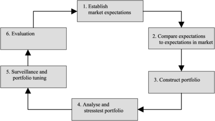
Table 3 Market expectations as of February 8th, 2002. In this particular run, 15 asset classes were used. The matrix illustrates the market expectations for each asset class in the “normal” state of the world. In addition to this matrix, the correlation matrix must be specified. Specifications for the “crash” state of the world are specified in the same way, in addition to the probability of the crash occurring. The expectations are given with a three month time horizon. Note that for money market and bond futures, the expectations are given on the interest rate level not returns

3. The portfolio construction is an iterative process as illustrated in Figure 9. The starting point is our market expectations. A large number of scenarios consistent with these expectations, typically a few thousand, are generated and visualized by histograms for each marginal distribution. See Figure 10 for an example of a return distribution. The team discusses the visualization, and more often than not, some expectations are changed when the team is confronted with the graphical representation of the expectations. When the generated scenarios are accepted, they are input to the TAA optimization model.

Fig. 9 The portfolio construction process.

Fig. 10 Visualization of the expected return distribution of Japanese equities. The histogram includes all scenarios, both from the “normal” and the “crash” state of the world. The skew of the distribution is 0.55, whereas the kurtosis is 3.61 (compared to 3 of the normal distribution).

Table 4 Optimal portfolio (in mill USD). Notice that the volatility of the return of each asset class varies substantially, see Table 3 for estimates. For instance, the volatility of equity futures can typically be 100 times larger than the volatility of the money market futures. That explains the large differences in magnitude of the positions

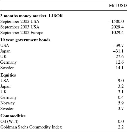
The TAA-model is run, and the optimal asset allocation mix is analyzed. As discussed in Section 2, experience has demonstrated that there are many asset allocation mixes that are almost equally as good in the sense that they provide approximately the same risk reward tradeoff. If we are not comfortable with the allocation mix, this is usually due to the market expectation input. We would therefore reevaluate some of the market expectations. However, if we believe market expectations are appropriate and we still dislike certain minor aspects of the optimal asset allocation, we will constrain the portfolio construction problem based on experience, even though the consequence is that the constrained optimization problem will find a portfolio with slightly worse risk reward tradeoff. An example can be to constrain the position in an asset class for which we lack conviction in our estimate for the expected return distribution (but where the estimate is still our best guess). It is important to notice, however, that the model decides the main structure of the portfolio, and that the subjective constraints only to a small extent influence that structure. From a modeling perspective, it is our belief that the error introduced by the subjective constraints is well within the error bound of the model itself. The (unconstrained) optimal portfolio given the market expectations partly described in Table 3 is shown in Table 4.

Clearly, it is possible to look at the profit or loss for the fund as a whole in order to measure it’s success. Evaluating the contribution from each member of the team is more difficult. But, since the market expectations are quantified and documented, and since they can, to some extent, be compared to what actually happened, we believe the evaluation process is of high quality and adds value. We are very careful not to base our evaluation on hindsight.

The incentive structure is related to the evaluation process. In building the incentive structure, the main goal has been to make sure that the incentives of the asset managers are in line with the incentives of the clients and also reflect the longer-term goals of the asset management company. The TAA-team as a whole has a performance related bonus and a bonus based on qualitative aspects. The challenge is to motivate the individuals by giving them credit for good work, but at the same time ensuring that the incentive system does not have a negative influence on the group decision process and creates internal conflicts.

5.1 Developing the models

Since contact was established late 1995 between the asset management team of Gjensidige-NOR and the authors of this paper, the focus for the project has evolved as follows:

After the initial work with the conceptual modeling framework for the ALM-problem, see Høyland and Wallace (2001a), we realized that the biggest challenge in terms of developing a model that would potentially be used for practical decision-making, was to construct adequate input to the model. This input had to be consistent with the judgmental views of the asset managers. In the financial industry there was, and still is, widespread skepticism regarding using asset allocation models. This is partly due to the fact that if managers have tried quantitative tools they have applied a mean-variance framework with the weaknesses discussed in Section 2.6. So, the first step was to agree upon how the judgmental views could be expressed. The conclusion to this step was that the asset managers wanted to express views on the return distribution of the asset classes directly, not on some common underlying factors that drove asset prices. Secondly, it was considered crucial to be able to express asymmetrical and potentially fat tailed distributions. After starting with a system where the users specified a marginal distribution by specifying a certain number of its percentiles, and derived the first four moments from these marginal distributions, the asset managers got used to, and became comfortable with, specifying the moments directly. See Høyland and Wallace (2001a) for more details on the work undertaken on the scenario generation methodology. From late 1997 and onwards, the strategic model was used as decision support for the ALM-planning of the life insurance company. The tactical asset allocation group was first established in 1998, and the TAA-model was then developed. As the TAA-group wanted to use the methodology on a more continuous basis, it became crucial to speed up the solution times. In particular, the scenario generation process was slow and a lot of effort was put into making efficient algorithms for solving the scenario generation problem, see Høyland, Kaut and Wallace (2003). Having speeded up the scenario generation process dramatically, the model could be used in a truly interactive way. The next focus was then to make the modeling system more user friendly.

The resources allocated to the project have been one full time PhD-student, plus additional resources from academia and Gjensidige-NOR. We believe one reason for the success of the project has been the ability to focus on the right issues at the right stages of the project. It is easy to get stuck on details and lose the “big picture” view in a project like this. An obvious reason why we have been able to avoid this is the very tight link between model developers and users. Involvement and commitment from the users have also secured that they have developed their thinking during the project and that they are familiar and comfortable with the concepts of the model.

5.2 Training and integrating employees

There are many different investment styles, or philosophies, for managing equity, bonds, and other kinds of assets. In one extreme, there are funds that are 100% dependent on one or a few star portfolio managers. In the other extreme, there are funds that can be run almost without any investment/market competence, for instance by making use of mechanical trading rules based on empirical prices. Clearly, funds that completely rely on one or a few star portfolio managers and their personal investment styles are vulnerable.

Asset managers compete for skilled labor, and will experience a certain turnover. For a fund it is therefore essential to have the ability to replace human competence smoothly, i.e., to be efficient in the process of educating and integrating new employees. Our experience in building the TAA-team is that the modeling framework has been very valuable in this respect. New employees are introduced to an established structured process. They will hopefully learn from the investment process, and in particular from the processes of generating market expectations. After observing from the sideline for a period, a new employee is allocated a responsibility and is forced to quantify market expectations. This normally creates motivation to develop a structured information collection and analyses process.

Different analysts will have different approaches in analyzing the markets. One extreme is the pure technician who bases expectations purely on historical price movements and overlooks economic fundamentals. Another extreme does not consider technical analysis at all, and bases expectations purely on fundamental analysis. In principle, the modeling framework we are describing does not exclude any analytical style. However, as a macro hedge fund, we are based on fundamental analysis. The group has developed a common platform that all the analysts apply, but within this platform, there are many different approaches to analyzing the markets, with differences in emphasis on different factors. The group believes that a variety of analytical styles is desirable.

5.3 The decision-making process

Consensus decision-making is generally a difficult task. The decision-making is not only about reaching a conclusion, but also a process where responsibilities have to be delegated and changed in a dynamic world. To ensure high quality decisions, it is important that consensus decision-making does not dilute responsibilities and remove possibilities for taking actions based on individual knowledge in special situations.

For consensus decision-making in portfolio management, an asset management group needs to agree both on market expectations and on the portfolio composition. As regards market expectations, the first step is to agree on which factors influence the portfolio composition. Should, for instance, asymmetry or fat tales in the return distributions be considered, and should a possible stock market crash be taken into account? Having reached agreement, consensus expectations can be established. Given consensus expectations, the next step is to agree on the portfolio composition.

For the problems we are discussing in this paper, the portfolio composition itself is a high dimensional and continuous optimization problem. Finding the potential profit positions and potential hedges can be difficult, and judging the magnitude of each position is even harder. In general, the group consensus process is made more complicated by differences among team members in both experience and their personal risk attitude. Due to these difficulties it is very common that investment funds are not based on consensus decision-making. Instead, the funds are often split into several sub-funds, which are run by individual fund managers.

We believe that the team consensus process is substantially simplified by using the modeling framework described in this paper. Its very existence forces the team members to see the full picture, and they all will have to be concerned, not only about their own input, but also that of the others. The portfolio construction itself is done by the TAA-model. Hence, the only consensus decisions are the market expectations. If there are disagreements regarding the quality of the portfolio, discussions will always have to revert to the data that produced the result.

There are, however, still challenges in the group consensus market expectation process. In particular, differences in experience and personal risk attitude can create imbalances in the expectation process. By the risk reward trade-off in the objective function of the TAA-model, a common risk attitude function for the group as a whole is established. However, all analysts have a feel for how the portfolio is constructed relative to the expectations. Hence, a risk averse analyst will be careful in presenting expectations that are likely to lead to large positions within “his” asset classes, while less risk averse analysts are more likely to seek such positions. The personal risk aversion levels for the members of the group are functions of both personal attitudes and experience. Due to such differences, the group has put a lot of emphasis on the process of calibrating the expectations.

When calibrating the expectations, much attention is given to the key expectations, which are the expectations for the return on global cash, bonds, equity and commodities, in addition to the ranking of the different regions within each asset class. A potential danger in this calibration process is that the senior group members dominate. However, the group accepts that there are differences in experience, and seeks to obtain a balance between influence and experience.

5.4 Organizational learning

The evaluation process was briefly discussed in the introduction to Section 5. Many traders use so-called trading plotters, where the reasoning behind a trade and the profit and loss taking levels are documented. With its quantitative approach, the TAA-team is naturally forced to do this documentation and all material from each TAA-meeting, including the analyses and the actual expectations, are collected. This is used to evaluate the performance from month to month and also to undertake a more comprehensive evaluation at the end of the year. Our belief is that systematic evaluation sharpens and motivates the members of the team and that this improves the quality of the investment process over time.

It may be useful to relate, briefly, the above discussions to organizational learning, see Huber (1991) for an overview. First, the knowledge acquisition here is mostly through performance monitoring. The organization keeps track of all its decisions with respect to investments, including the basis for the decisions, and the financial results. That way, it is possible to understand, ex post, why a certain decision was made, and hopefully learn, irrespective of the outcome. In particular, this way of keeping records will help avoid hindsight taking the front seat in the learning process. It is a well-known phenomenon that, ex post, all humans seek to explain what happened. Fischhoff (1982) calls this creeping determinism. It is hard to accept that an outcome was random, and that something else could have happened as well. Notice that a good decision can lead to a negative result, simply because of bad luck. Good records will not automatically overcome this problem, but it is a necessary basis for proper learning about random phenomena.

5.5 Track record

In July 1999, a separate portfolio, with positions based on the TAA-model, was established. Figure 11 shows the performance of the fund since the start up. The accumulated excess return from startup to the end of April 2002 is 5.60%. The risk, measured by annualized ex post tracking error (one standard deviation of excess monthly returns), is 1.71%. This gives an average information ratio⁴ of approximately 1.19 each year.

Fig. 11 Track record.

The risk limit for the fund has been 5% in tracking error (one standard deviation of annual excess returns). The fund has been run for Gjensidige-NOR Spareforsiking and Gjensidige-NOR Forsikring (the Life and Non-Life insurance companies), and the capital base has been 7.5 billion NOK, equivalent to more than 800 million USD, since May 2000.

The fund applies a pure overlay strategy, meaning that only derivatives are used to construct the bet structure. This implies that the underlying funds can be invested in any benchmark, for instance, S&P 500 or Norwegian money market. Hence, for measuring the performance of the fund, the choice of benchmark is not important. The derivative activities generate an excess return. The total return for the client will be the return on the benchmark (whatever that is) plus the excess return generated from the derivative strategies.⁵

The risk profile of the fund has been modest relative to other funds with a similar macro hedge fund style. Since the fund has been used to run the tactical asset allocation for the Life and Non-Life companies (both running a moderated balance risk), we have chosen to run the fund with a large capital base and low risk. It is the relative risk multiplied by the capital base that will be relevant for the results. For example, if the capital base had been defined to be 750 million NOK instead of 7.5 billion, the excess return and the tracking error would have been 56 and 17.1%, respectively, instead of 5.6 and 1.71%. To evaluate the result we need to consider the information ratio and the shape of the actual return distribution. Figure 12 shows a histogram of the monthly returns since startup. Notice that the histogram is skewed to the right. The five highest monthly returns in absolute value are positive, and there are nine observations with a higher return than 0.5%, whereas only one observation with a lower return than . The number of observations is low, but it appears that the group has been able to construct an asset allocation—which is consistent with the goal of optimization—to create a right skewed return distribution.

Fig. 12 Histogram of monthly excess returns. The lowest monthly return is −0.67%, whereas the highest is 1.46%.

Our track record indicates ability to generated excess return even though the number of observations is too low to claim this with any statistical significance. Of course, it is possible the results are due to pure luck—it is hard to judge. If it is not pure luck we need to justify why we are able to generate this excess return—what market inefficiencies are we exploiting?

The motivation for the modeling framework comes from what the TAA-team believes to be the two key sources of potential excess return (i.e., return in excess of a benchmark return):

There are of course other sources of excess return, such as market timing, arbitrage opportunities and dynamic utilization of risk limits (as well as luck and chance), but we believe that our own market expectations and the portfolio construction are the two most important elements. Most portfolio managers are subjective/judgmental on both elements. Hence, the decisions made are a mixture of judgmental views on the market and a judgmental view on how to create a portfolio consistent with the market expectations. Within the modeling framework we have described, we are still judgmental on market expectations, but we run a tactical asset allocation model to create a portfolio that is consistent with our own market expectations.

We believe that there are particularly large inefficiencies across asset classes, whilst there may be lesser inefficiencies within asset classes. This is partly caused by the prevailing industry standard of having sector specialists who do not look at bets mixing asset classes. As have been highlighted in this paper, the TAA-group is mostly betting on the relationships among classes and not within classes.

To remove inefficiencies among classes, there must be some players in the market filling the gaps. But this requires appropriate tools, as it is impossible for a human brain to get a proper overview over the effect of bets in light of all correlations and lacks of normality. And few have these tools. This is where we believe we have an advantage.

References

D. Bell. Risk, Return and utility. Management Science. 1995;41:23-30.
J. Birge, F. Louveaux. Introduction to Stochastic Programming. Heidelberg: Springer; 1997.
D.R. Cariño, W.T. Ziemba. Formulation of the Russell–Yasuda financial planning model. Operations Research. 1998;46(4):443-449.
V.K. Chopra, W.T. Ziemba. The effect of errors in means, variances and covariances on optimal portfolio choice. Journal of Portfolio Management. 1993;19:6-11.
G. Consigli, M.A.H. Dempster. Dynamic stochastic programming for asset–liability management. Annals of Operations Research. 1998;81:131-161.
A. Consiglio, F. Cocco, S.A. Zenios. The value of integrative risk management for insurance products with guarantees. The Journal of Risk Finance. 2001:6-16. Spring
P.E. de Lange, S.-E. Fleten, A.A. Gaivoronski. Modeling financial reinsurance in the casualty insurance business via stochastic programming. Journal of Economic Dynamics and Control. 2004;28(5):991-1012.
Dert, C.L., 1995. Asset liability management for pension funds, a multistage chance constrained programming approach, PhD thesis. Erasmus University, Rotterdam, The Netherlands
J. Dupacova. Output analysis for approximated stochastic programs. In: S. Uryasev, P.M. Pardalos, editors. Stochastic Optimization: Algorithms and Applications. Kluwer; 2001:1-29.
J. Dupacova, G. Consigli, S.W. Wallace. Generating scenarios for multistage stochastic programs. Annals of Operations Research. 2000;100:25-53.
B. Fischhoff. For those condemned to study the past: heuristics and biases in hindsight. In: D. Kahneman, P. Slovic, A. Tversky, editors. Judgment under Uncertainty: Heuristics and Biases. Cambridge University Press; 1982:335-351. Chapter 23
A.A. Gaivoronski, P. De Lange. An asset liability management model for casualty insurance companies: Complexity reduction versus parameterized decision rules. Annals of Operations Research. 2000;99:227-250.
Gaivoronski, A.A., Høyland, K., De Lange, P., 2000. Statutory regulations of casualty insurance companies: An example from Norway with stochastic programming analysis. In: Uryasev, S., Pardalos, P.M. (Eds.), Stochastic Optimization: Algorithms and Applications, pp. 53–83
Geyer, A., Herold, W., Kontriner, K., Ziemba, W.T., 2002. The Innovest Austrian Pension Fund Financial Planning Model InnoALM, Working paper. University of British Columbia
G.P. Huber. Organizational learning: The contributing process and the literatures. Organizational Science. 1991;2(1):88-115.
K. Høyland, M. Kaut, S.W. Wallace. A heuristic for moment-matching scenario generation. Computational Optimization and Applications. 2003;24:169-185.
K. Høyland, S.W. Wallace. Generating scenario trees for multistage decision problems. Management Science. 2001;47:295-307.
K. Høyland, S.W. Wallace. Analyzing legal regulations in the Norwegian life insurance business using a multistage asset liability management model. European Journal of Operational Research. 2001;134:293-308.
J.C. Jackwerth, M. Rubinstein. Recovering probability distributions from option prices. Journal of Finance. 1996;51(5):1611-1631.
P. Jorion. Risk management lessons from long-term capital management. European Financial Management. 2000;6:277-300.
P. Kall, S.W. Wallace. Stochastic Programming. Chichester: Wiley; 1994.
J.G. Kallberg, W.T. Ziemba. Comparison of alternative utility functions in portfolio selection problems. Management Science. 1983;XXIX:1257-1276.
R. Kouwenberg, S.A. Zenios. Stochastic programming models for asset liability management. Handbook of Asset Liability Management, Vol. A: Theory and Methodology. Handbooks in Finance, North-Holland, 2006:253-303.
B.G. Malkiel. A Random Walk Down Wall Street, eighth ed. New York: W.W. Norton & Company; 2003.
H. Markowitz. Portfolio selection. Journal of Finance. 1952;7(1):77-91.
H. Markowitz, E. van Dijk. Risk-return analysis. Handbook of Asset Liability Management, Vol. A: Theory and Methodology. Handbooks in Finance, North-Holland, 2006.
J.M. Mulvey. Generating scenarios for the Towers Perrin investment system. Interfaces. 1996;26:1-13.
L. Rahl, editor. Risk Budgeting, A New Approach to Investing. London: Risk Books, 2000.
1 On 4 December, 2003, Gjensidige-NOR and DnB merged to create DnB NOR which became Norway’s largest financial group.
2 Theoretically the zero benchmark return is too low because the TAA group will use risk capacity of the life insurance company, which should be compensated. Hence, the benchmark return should be risk adjusted to a positive number. However, this issue is of more importance when discussing the incentive structure between the TAA group and the life insurance company, since adjusting the benchmark return would not change the important characteristics of the utility function.
3 This is under the assumption of an asymmetrical utility function for which we argued in Section 2.1.
4 The information ratio is the excess return divided by the standard deviation of the excess return.
5 The model implication is that the shortfalls (outcomes that generates a negative contribution to the objective function value) will be measured relative to zero. For a cash portfolio, where the cash is allocated to the different asset classes, the shortfalls would be measured relative to the return on a specific benchmark.
6 With this motivation for the modeling framework, the efficient market theory is abandoned. For a comprehensive discussion on market efficiency, see Malkiel (2003) and the references therein.