
Handbook of Asset and Liability Management, Vol. 2, No. suppl (C) • 2007
ISSN: 1872-0978
doi: 10.1016/S1872-0978(06)02012-6
Chapter 12 Dynamic Financial Analysis for Multinational Insurance Companies*
Abstract
Global insurance/reinsurance companies can gain significant advantages by implementing an enterprise risk management system. The major goals are: (1) increase long-term profitability, (2) reduce enterprise risks, and (3) identify the firm’s optimal capital structure. Profitability depends upon evaluating uncertainties as a function of a set of common factors across the enterprise. The system takes up all major decisions: identifying optimal liability-driven asset strategies, expanding/contracting insurance lines and pricing policies, constructing sound reinsurance treaties, and setting the firm’s capital structure. To implement risk management in global companies we present a decentralized system. An automated toolkit eases constructing an enterprise system (Appendix A). Real-world experiences are highlighted via case studies.
Keywords
• dynamic financial analysis • enterprise risk management • asset and liability management • stochastic programs • optimizing insurance companies
JEL classification
• C61 • D81 • G11 • G22
1 Introduction to dynamic financial analysis
Leading financial companies have begun to integrate their strategic decisions within enterprise-wide planning systems. The underlying modeling concepts are identified by several terms depending upon the context, including total integrated risk management (TIRMTM), dynamic financial analysis (DFA), enterprise risk management (ERM), and asset and liability management (ALM). We employ the DFA name in this paper, given our emphasis on applying the technology to insurance companies. Each title portrays a shift in emphasis and agenda; DFA focuses on financial risks/analysis, while ERM includes operational and other non-financial sources of risks. The overall goals are similar—to improve a company’s economic performance by collecting, analyzing, and managing information regarding the primary risk and return factors. Once the risks and rewards are properly identified, company executives can take actions to maximize the firm’s shareholder value.
The primary areas of application for DFA in an insurance company are: (1) asset allocation strategies, (2) business decisions regarding the lines of insurance to underwrite, (3) pricing strategies, (4) reinsurance deals, (5) capital allocation, and (6) setting target rates of return. Important firm-wide decisions of the chief executive, chief financial officer and other executives can be evaluated by means of a strategic DFA system. Likewise, operational decisions such as underwriting policy can be improved by means of coordinated risk management. We suggest that lower level decisions should be accommodated within tactical risk management systems, which are linked to the strategic DFA system (see Section 4). In this report, we emphasize the strategic nature of DFA.
What motivates a company to implement an integrated risk management system? First, there have been spectacular failures despite the steep regulations for insurance companies, for example, Equitable Life in the United Kingdom. These failures show that current regulations do not ensure the solvency of an insurance company. Part of the failure can be attributed to organizational and competitive issues, such as periods of industry-wide under-pricing practices. But also, the failure can be attributed to the lack of modern risk management systems. Legacy systems often employ historical data for estimating losses, for example, without regard for the factors that drive the risks. This approach can underestimate the rare events since most economic and physical risks do not fit the normal distribution in the tails. See Section 2 for further details on this point.
Importantly, there is recognition that a modern insurance company can increase its profits by careful analysis of the sources of its risks, intelligent pricing strategies, and by diversifying away from the convergent risks. As an example, by growing an international business, e.g., AIG, or by limiting exposure to the factors giving rise to the rare events, e.g., Renaissance Reinsurance (Lowe and Stanard, 1996), and Smartwriter at St. Paul, a company can reduce the amount of capital needed to support a fixed level of business (Berger, Mulvey and Nish, 1998). Risk-adjusted profits increase through these strategies. In this paper, we differentiate the traditional static valuation methods from dynamic methods for valuing the activities of the firm. Section 4 describes an approach for deriving a dynamic valuation in the context of a decentralized DFA approach.
There have been several key successful applications of the DFA methodology. The Frank Russell Company developed one of the early DFA systems, for the Yasuda PC Company in Japan (Cariño et al., 1994; Cariño, and Ziemba, 1998). This implementation has been widely cited in the literature. Other examples include: Tillinghast–Towers Perrin (Mulvey, Gould and Morgan, 2000), Renaissance Reinsurance (Lowe and Stanard, 1996), American Re-insurance (Berger and Madsen, 1999), Swiss Re (Laster and Thorlacius, 2000), the Norwegian life insurance company Gjensidige (Hoyland, 1998), and recently AXA. In the last and other examples, a significant issue involves calculating the target capital to deploy across its worldwide operations. While conducting independent analyses for each of its global subsidiaries, AXA aggregates its businesses in order to calculate the overall diversification benefits. These results provide better information regarding the safety of the organization in conjunction with the desired level of capital to maintain.
Other industries have made progress on improving efficiency through integrated decision-making and optimization. As a prominent example, the area of integrated logistics has benefited by real time information flows across the supply chain—from sales source backward to the distributor, the warehouse locator, the transportation system, and the manufacturer. Each part of the organization is aware of its role and especially the costs of delays and inefficient operations. For example, inventory allows a company to service the customer quickly, but it comes at a high price in terms of flexibility to change the product mix. Dell Computer provides a prototypical example of minimizing inventory—building their computers to exact customer specifications. Many process and manufacturing companies now deploy the enterprise technology, including AspenTech, IBM, I2 Technologies, etc. See Geoffrion and Krishnan (2001), Erkan (2006) and Lin et al. (2000). These industries directly benefit by applying enterprise-focused technology to improve efficiency. Employees enhance value by improving the quality of information on which decisions are based.
An insurance company’s capital can be treated as inventory—but with a dual purpose. First, the capital serves to reduce risks of adverse consequences; it is a buffer to keep the firm solvent and to maintain a positive credit rating. Second, the capital forms a part of the asset base in which investment returns occur. As interest rates and inflation rates have dropped since 1980 with an accompanying increase in stock and fixed income asset returns, the importance of investment income has increased (Enz, and Karl, 2001; Consiglio and Zenios, 2001). However, insurance companies are unlikely to experience the same investment climate over the next few years and, therefore, a modern insurance company will need to improve its underwriting results in order to gain a respectable return on equity. The capital structure plays an important role in determining the enterprise’s risks and rewards.
There are several primary goals for an integrated risk management system: (1) to grow the company’s capital with the optimal risk adjusted rate, (2) to ensure that the company survives a series of adverse circumstances, and (3) to improve the firm’s profitability by increasing efficiency and making comparable decisions regarding risk and reward. Taken together, these goals are synonymous with “maximizing shareholder value”.
In the next section, we describe the major components of an enterprise risk management system. The three primary elements consist of: (1) a stochastic scenario generator, (2) a corporate simulator, and (3) a module for identifying improving decisions and processes. Each element builds on the previous (Figure 1).

A DFA system depends, first of all, on modeling the important economic uncertainties—interest rates, inflation, stock returns, insurance losses, bond returns. This module, the “scenario generator”, consists of stochastic differential equations for each of the economic factors, asset returns, and the liability (insurance related) cash flows. The scenario generator provides inputs for the decision simulator. The model evaluates selected policy/decision rules across each of the scenarios—thus simulating the company as it reacts to the uncertainties embedded in the scenarios. Policy rules should reflect a reasonable approximation of the company’s business strategy in the face of changing economic and business conditions. Under each scenario, the company will achieve a specified performance. The set of performance indicators across the scenarios completes the decision simulator. As with any stochastic model, the results depict probability distributions of outcomes. Temporal issues complicate the problem by adding performance measures at various time periods.
The remainder of this report is organized as follows. The DFA model is defined in the next section, including a discussion of the scenario generator and the optimization algorithms available for solving the resulting model. The search for an optimal solution is hindered due to the presence of sampling errors, the possibility of a non-convex objective function, and the need for multiple goals depending upon the stakeholders’ positions. Section 3 describes a series of case studies in which the DFA system can improve decision-making. Prominent examples include: asset allocation strategies, selection of business activities to increase or decrease, the structure of reinsurance treaties, and the company’s degree of leverage (gearing). Since many of these decisions interact with each other, we suggest that the full system be run in an integrated fashion. In Section 4, we show that the DFA system can be implemented in large, decentralized companies by extending existing capital allocation policies. The scenario approach lends itself well to the decentralized management, common in most multinational financial organizations. Last, we make recommendations for future developments in the DFA arena (Section 5).
Appendix A discusses the use of software tools to build and maintain a complex DFA modeling system. Since an integrated system must address the major elements of an insurance company, there are numerous sources of data and estimation, requiring a series of underlying assumptions throughout the process. We have found that the efficient design of a DFA software system requires a DFA toolkit in which the system is easy to use, flexible, and can be customized by the user to accommodate the complex structure of many insurance products. Also, users should be able to quickly pinpoint the underlying assumptions. An example of a DFA toolkit is shown in Appendix A.
2 Basic structure of a DFA system
An expanded version of a strategic DFA system is shown in Figure 2. The first issue involves setting the planning period. Typically, the DFA model projects the company over the next 3 to ![]() years, with annual or possibly quarterly time periods. The firm’s position is evaluated at the end of the planning period—the horizon. Special attention is paid to the next year’s profit and surplus, of course, along with the risk of a downgrade in credit quality and other short-term indicators. The company’s stock price and future well-being depend upon these performance indicators. The definition of risk measures and related aspects of the objective function are discussed below.
years, with annual or possibly quarterly time periods. The firm’s position is evaluated at the end of the planning period—the horizon. Special attention is paid to the next year’s profit and surplus, of course, along with the risk of a downgrade in credit quality and other short-term indicators. The company’s stock price and future well-being depend upon these performance indicators. The definition of risk measures and related aspects of the objective function are discussed below.

Fig. 2 The basic structure of an integrated risk management system. The planning period (t=1,2,…,T).
The scenario generator projects a series of plausible paths over the multi-period planning horizon (step 1). Scenarios are consistently modeled across the organization; the behavior of the assets and the liabilities comes from the same factors. Given a set of policies, we simulate the corporation over each scenario (step 2). The company’s overall financial health is ascertained with regard to the pre-determined goals. Last, an optimal search procedure (step 3) is implemented in order to find a set of policies that optimize the company’s shareholder value. As there are numerous choices of goals facing insurance executives, the optimizing search must necessarily engage the judgments of the senior managers. The problem fits the domain of multi-objective optimization. In this section, we describe the DFA model at a relatively high level.
2.1 Scenario generators
Financial simulation requires a consistent method for projecting the random variables over the multi-period planning horizon. The scenario generators are critical for analyzing the insurance company in an integrated fashion, for example, when evaluating the merger of financial and insurance risks. Actuaries, financial planners and insurance executives actively employ stochastic generators. An early economic generator in the UK is the Wilkie model (1987). Mulvey (1989) developed a system for Pacific Mutual and latter for Towers Perrin–Tillinghast (1996, 1998). These generators possess a cascade structure with a nonlinear relationship among the factors. Alternatively, firms have developed linear systems such as vector auto-regressive models.
There are three key steps when building a scenario-generating module: (1) defining the modeling equations, (2) estimating the parameters, and (3) sampling the system. First, we discuss the model equations. Herein, Figure 3 depicts an important issue that arises when generating scenarios—the close connection between the underlying economic factors and both the assets returns and changes in the liability cash flows. Interest rate changes will impact asset returns (for fixed income asset categories) and the discount rate for valuing liabilities. Linking the assets and liabilities in a consistent fashion requires modeling the driving factors, in this case interest rates. The structural approach begins with modeling the economic and monetary factors, especially interest rates, inflation, GDP, corporate earnings, and credit spreads, over the multi-period horizon. As we will see, interest rates are generally modeled by means of mean reverting diffusion equations; bond returns are a direct function of interest rate swings due to changing economic conditions. The calibration of the parameters is complicated, and approaches such as maximum likelihood must be extended. Among others, methods of indirect inference apply to the resulting calibration problem; see Duffie and Singleton (1993), Berger and Madsen (1999), Gourieroux, Monfort and Renault (1993), Mulvey, Rosenbaum and Shetty (1999), and Chen and Bakshi (2001) for differing approaches. Also, see Hoyland and Wallace (2001) for a practical method for generating scenarios over a stochastic programming tree.

Fig. 3 The relationship of underlying factors to assets and liability cash flows, valuations, and returns.
We depict uncertainty by a set of discrete realizations ![]() . The projection module is based on a continuous set of stochastic differential equations, as defined by
. The projection module is based on a continuous set of stochastic differential equations, as defined by ![]() . To give an illustration, we describe the nominal interest rate process within a real-world DFA system—the CAP:Link scenario generator. This scenario generator has been implemented throughout the world for pension plans and insurance companies (Mulvey, Gould and Morgan, 2000).
. To give an illustration, we describe the nominal interest rate process within a real-world DFA system—the CAP:Link scenario generator. This scenario generator has been implemented throughout the world for pension plans and insurance companies (Mulvey, Gould and Morgan, 2000).
The CAP:Link interest rate model is a spot rate model that is derived in a three-stage process. The first stage is a pair of linked stochastic processes. We assume that long and short interest rates link together through a correlated white noise term and by means of a stabilizing term that keeps the spread between the short and long rates under control.
Define short and long nominal interest rates (spot rates) as follows:
where
| short interest rate | |
| long interest rate | |
| the short and long interest rates increments over dt | |
| the spread between long and short interest rates | |
| correlated standard Brownian motions (white noise terms) | |
| drift on short and long interest rates | |
| drift on the spread between long and short interest rates | |
| instantaneous volatility | |
| mean reversion level of short rate | |
| mean reversion level of long rate | |
| mean reversion level of the spread between long and short interest rates |
Among them, ![]() ,
, ![]() ,
, ![]() ,
, ![]() ,
, ![]() ,
, ![]() ,
, ![]() ,
, ![]() ,
, ![]() are unknown parameters.
are unknown parameters.
The second stage models a third point on the curve—mid-point. The equation for the mid rate is
where
and where
| mid interest rate | |
| the mid interest rate increments over dt | |
| standard Brownian motion (the white noise term) | |
| drift on mid interest rate | |
| instantaneous volatility | |
| exponential weight between long and short interest rates |
Among them, ![]() are parameters.
are parameters.
The mid-point accounts for curvature shifts in the yield curve.
In stage three we fill out the spot yield curve using a smoothing procedure:
where ![]() ,
, ![]() and T is the maturity of the long interest rates. Given parameters
and T is the maturity of the long interest rates. Given parameters ![]() and
and ![]() , this equation is linear, leading to a quick solution. These parameters do not generally change as a result of a re-calibration of the model. The interest rate submodel is defined in terms of the indicated twelve parameters.
, this equation is linear, leading to a quick solution. These parameters do not generally change as a result of a re-calibration of the model. The interest rate submodel is defined in terms of the indicated twelve parameters.
The second element in building a scenario generator involves parameter estimation. When calibrating the model we weigh the competing needs of the users. For instance, there is a need to model accurately the covariance structure of interest rates at relatively high frequency (monthly), as some insurance contracts are sensitive to term spread and volatility of changes in bond yields. Other contracts have longer-term interest rate guarantees and are more sensitive to the range of interest rates over longer (10 to 20 year) periods. The calibration targets relate to both bond yield characteristics and bond return characteristics.
Targets are set for:
The relationships of other random variables within the CAP:Link system are displayed in Figure 4. For example, price inflation is projected in conjunction with the nominal interest rates, and as a consequence, the real (nominal minus inflation) government spot rate curve is derived as part of the process.

DFA models require a rich set of economic factors in the economic scenario generators, to adequately cover the range of risks encountered by insurance and other financial institutions. The US Society of Actuaries and US Casualty Actuarial Society are currently advocating a publicly available model to include the following variables:
The third stage is to perform a sampling exercise in order to select scenario set ![]() . There are several alternative sampling procedures; see references: Consigli and Dempster (1998), and Rush et al. (2000). The goal is to generate scenarios that minimize the sampling errors and lead to robust recommendations. Variance reduction methods can be applied as appropriate. The number of scenarios depends on the usage of the DFA system. For example, insurance companies require more precision than pension plans and accordingly a greater number of scenarios. It is not uncommon for a DFA model to employ 10,000 to 100,000 or more scenarios so that capital allocation decisions can be based on the DFA system.
. There are several alternative sampling procedures; see references: Consigli and Dempster (1998), and Rush et al. (2000). The goal is to generate scenarios that minimize the sampling errors and lead to robust recommendations. Variance reduction methods can be applied as appropriate. The number of scenarios depends on the usage of the DFA system. For example, insurance companies require more precision than pension plans and accordingly a greater number of scenarios. It is not uncommon for a DFA model to employ 10,000 to 100,000 or more scenarios so that capital allocation decisions can be based on the DFA system.
The scenario generator module provides a foundation for the remainder of the DFA system—the corporate simulator and later the optimizer. Thus, company users should pay close attention to the scenarios coming out of the module. Some questions to ask: Are the resulting scenario paths sensible? See Figure 5 for a graph of short and long interest rates and inflation. Do the asset returns link to the underlying economic factors in a consistent fashion? For example, are bond returns derived from interest rate changes, especially the spot rate and yield curves? What are the summary statistics of the generated scenarios? Does the model include an adequate number of scenarios with tail events, such as recessions or yield curve inversions?
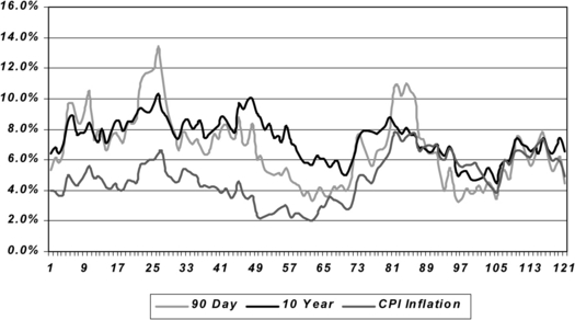
Fig. 5 Examples of interest rates and inflation over 10 year planning period (yield curve inversion occurs at two periods—months 25 and 86).
Scenario generators are established in the insurance liability arena. An important example involves estimating the probability of loss for covered properties under projected catastrophic events—mostly hurricanes and earthquakes. These stochastic generators play a critical function when insurance companies and state regulators approve insurance prices. Running these models helps in calculating a company’s capital requirements. Insurance companies routinely evaluate their books of business with the catastrophic simulation models (from AIR, RMS, and EQE international, among others). 10,000 to 100,000+ scenarios must be generated due to the large number of possible events and the resulting severe consequences and low probabilities for large losses (Bowers, 2002). Strikingly, the scenarios display losses with highly non-normal tail properties, i.e., high severity and low probabilities with highly skewed left tailed loss distributions (Mulvey and Erkan, 2006).
An emerging area for scenario generation entails weather-related projections and topics such as degree-days above or below average for selected locations and time-periods. This application will expand along with new weather-linked securities and derivatives as financial companies introduce products for hedging energy costs by energy producers and consumers. The growth of this market hinges on well-conceived, trustworthy scenarios for risk management.
Constructing a scenario generator requires attention to three key issues: (1) the realism of the model equations, (2) calibration of the parameters, and (3) procedures to extract the sample set of scenarios, the projection systems should be evaluated with historical data (back-testing), as well as on an ongoing basis. Confidence in these systems will continue only if they display a sufficient degree of accuracy. Research is needed in this area, especially with regard to points 1 and 2 above.
2.2 Enterprise simulators
The simulation module mimics the insurance company’s decisions over the planning period for each of the presented scenarios. An insurance company, for example, makes decisions regarding their asset mix, business strategies for growing or shrinking their insurance lines, and the firm’s capital structure (leverage, exposure, etc.). An insurance executive sets investment strategies along with policy for capital contributions, business expansion, etc. These decisions involve tax and other regulatory implications. The investment process consists of ![]() time stages. The first decision juncture represents the current date. The end of the period, T, the planning horizon, may depict a point in which the company has some critical planning purpose, such as the repayment date of a substantial liability, or more likely a point in the future consistent with the company’s plans. A substantial portion of the simulation involves modeling the regulatory requirements including Statutory and GAAP positions, and the accompanying constraints on capital allocation. Due to the regulatory burden, it is difficult to operate solely on economic grounds. Thus, there is a need for a separate set of constraints and variables for the statutory, accounting and tax rules. See references (Burket, McIntyre and Sonlin, 2001; Cariño and Ziemba, 1998; Hoyland, 1998; Kaufman and Ryan, 2000; and Lowe and Stanard, 1996) for detailed discussions of the regulatory environment for insurance companies and other modeling complications.
time stages. The first decision juncture represents the current date. The end of the period, T, the planning horizon, may depict a point in which the company has some critical planning purpose, such as the repayment date of a substantial liability, or more likely a point in the future consistent with the company’s plans. A substantial portion of the simulation involves modeling the regulatory requirements including Statutory and GAAP positions, and the accompanying constraints on capital allocation. Due to the regulatory burden, it is difficult to operate solely on economic grounds. Thus, there is a need for a separate set of constraints and variables for the statutory, accounting and tax rules. See references (Burket, McIntyre and Sonlin, 2001; Cariño and Ziemba, 1998; Hoyland, 1998; Kaufman and Ryan, 2000; and Lowe and Stanard, 1996) for detailed discussions of the regulatory environment for insurance companies and other modeling complications.
The modeling problem becomes complicated when the value of the liability cash flow is a direct function of the asset returns and the company’s annual decisions on crediting and payouts. This linkage occurs in life insurance. In this case, the resulting simulation system must be designed to closely link the asset allocation with the company’s crediting policies. Asset and liability decisions are made in a coordinated fashion.
Next, we define the DFA model as a multi-stage stochastic program. The underlying approach builds upon the model in Mulvey, Correnti and Lummis (1997), with special attention to managing the asset and liability decisions within an insurance environment.
First, we divide the planning horizon ![]() into two discrete time intervals
into two discrete time intervals ![]() and
and ![]() , where
, where ![]() and
and ![]() . The former corresponds to periods in which investment decisions are made. Period T defines the date of the planning horizon; we focus on the company’s position at the beginning of period T. Decisions occur at the beginning of each time stage. Much flexibility exists. At the tactical level, an active bond trader might see his time interval as short as minutes, whereas the CEO will focus on longer planning periods such as the next Board of Director’s meeting. It is possible for the time steps to very-short intervals at the beginning of the planning period and longer intervals towards the end.
. The former corresponds to periods in which investment decisions are made. Period T defines the date of the planning horizon; we focus on the company’s position at the beginning of period T. Decisions occur at the beginning of each time stage. Much flexibility exists. At the tactical level, an active bond trader might see his time interval as short as minutes, whereas the CEO will focus on longer planning periods such as the next Board of Director’s meeting. It is possible for the time steps to very-short intervals at the beginning of the planning period and longer intervals towards the end. ![]() handles the horizon at time T by calculating economic and other factors beyond period T up to period τ. The investor does not render any active decisions after the end of period T.
handles the horizon at time T by calculating economic and other factors beyond period T up to period τ. The investor does not render any active decisions after the end of period T.
Asset investment categories are defined by set ![]() , with category 1 representing cash. The remaining assets can include broad investment groupings such as stock subindices, fixed income groups, and real estate. The categories should track well-defined market segments. Ideally, the co-movements between pairs of asset returns would be relatively low so that diversification can be done across the asset categories. Most insurance companies require many fixed income asset categories due to the nature of the business and the underlying degree of financial leverage.
, with category 1 representing cash. The remaining assets can include broad investment groupings such as stock subindices, fixed income groups, and real estate. The categories should track well-defined market segments. Ideally, the co-movements between pairs of asset returns would be relatively low so that diversification can be done across the asset categories. Most insurance companies require many fixed income asset categories due to the nature of the business and the underlying degree of financial leverage.
The business activities, mostly insurance products, are designated by the set ![]() . In many cases, we reference the insurance lines as separate activities. Depending upon the level of detail, we might aggregate multiple lines into a single j variable, or the aggregation can project common lines across geographical areas. The main feature is to be able to ascertain the losses with regard to the business activity, as a function of scenarios and time period. For this paper, we place the reinsurance decisions within a distinct activity (i.e., on the liability side of the balance sheet despite the fact that the resulting cash flows resemble asset categories).
. In many cases, we reference the insurance lines as separate activities. Depending upon the level of detail, we might aggregate multiple lines into a single j variable, or the aggregation can project common lines across geographical areas. The main feature is to be able to ascertain the losses with regard to the business activity, as a function of scenarios and time period. For this paper, we place the reinsurance decisions within a distinct activity (i.e., on the liability side of the balance sheet despite the fact that the resulting cash flows resemble asset categories).
A second partition of the enterprise tracks the profits and losses of distinct entities, called business units or alternatively divisions. The business units are identified by the symbol ![]() ; we include a variety of decompositions within this identifier. For example, we might separate the company into two divisions: (1) the US insurance company, and (2) the European insurance company. Accordingly, we associate all of the assets and the liabilities to one of these two divisions, within a mutually exclusive and collectively exhaustive partition. Thereby, we evaluate the company in two distinct ways—by asset and liability (insurance products) categories and by distinct divisions. If a company maintains their assets without regard to the liabilities, we generally employ a basket of assets that represents the current asset mix. Of course, any matching of assets to activities is allowed from the modeling standpoint. It is natural to subdivide the enterprise according to accounting and regulatory boundaries since the divisional context will be employed for calculating profit and losses. For our model, we assume that the income statement can be calculated as a function of the decision variables (x, y, etc.) This part of the simulation can be rather complex due to insurance rules and regulations and therefore outside the domain for this exposition. Nevertheless, we assume that profits and losses can be calculated for each division as a function of the decision variables:
; we include a variety of decompositions within this identifier. For example, we might separate the company into two divisions: (1) the US insurance company, and (2) the European insurance company. Accordingly, we associate all of the assets and the liabilities to one of these two divisions, within a mutually exclusive and collectively exhaustive partition. Thereby, we evaluate the company in two distinct ways—by asset and liability (insurance products) categories and by distinct divisions. If a company maintains their assets without regard to the liabilities, we generally employ a basket of assets that represents the current asset mix. Of course, any matching of assets to activities is allowed from the modeling standpoint. It is natural to subdivide the enterprise according to accounting and regulatory boundaries since the divisional context will be employed for calculating profit and losses. For our model, we assume that the income statement can be calculated as a function of the decision variables (x, y, etc.) This part of the simulation can be rather complex due to insurance rules and regulations and therefore outside the domain for this exposition. Nevertheless, we assume that profits and losses can be calculated for each division as a function of the decision variables:
where ![]() is the vector of key performance indicators and the decisions are set in the asset and liability space (
is the vector of key performance indicators and the decisions are set in the asset and liability space (![]() ), whereas the profit/loss results,
), whereas the profit/loss results, ![]() , are taken in the divisional space
, are taken in the divisional space ![]() . The
. The ![]() function encompasses technical issues, such as computing taxes, reserving for expected losses, addressing fixed versus variable costs, etc. We do not wish to minimize this part of the simulation, but the extent of the accounting rules and other regulations would overwhelm the statement of the basic DFA model. In addition at times, we may adjust the profit/loss values in order to improve the performance measures for example by engaging in reinsurance treaties (Section 4). The overall profit for the enterprise comes from summing the divisions’ profits:
function encompasses technical issues, such as computing taxes, reserving for expected losses, addressing fixed versus variable costs, etc. We do not wish to minimize this part of the simulation, but the extent of the accounting rules and other regulations would overwhelm the statement of the basic DFA model. In addition at times, we may adjust the profit/loss values in order to improve the performance measures for example by engaging in reinsurance treaties (Section 4). The overall profit for the enterprise comes from summing the divisions’ profits:
We assume that the company’s profit/loss is evaluated at the end of each period, using the enterprise as defined at the beginning of the period, with the results occurring over the reference time span. For convenience, we also assume that the cash flows are reinvested in the generating asset category and all the borrowing is done on a single period basis. This assumption can be readily dropped in an actual implementation.
For each ![]() ,
, ![]() , and
, and ![]() , we define the following parameters and decision variables. The elemental decision variables, such as asset allocation and business activity, refer to the state of the company at the beginning and during the time period.
, we define the following parameters and decision variables. The elemental decision variables, such as asset allocation and business activity, refer to the state of the company at the beginning and during the time period.
Parameters
| Total return for asset i, time period t, under scenario s (projected by the stochastic scenario generator as discussed). | |
| Probability that scenario s occurs, |
| Economic capital (wealth) in the beginning of time period 0. | |
| Transaction costs incurred in rebalancing asset i at the beginning of time period t (symmetric transaction costs are assumed, i.e., cost of selling equals cost of buying; comparable parameter for liabilities |
Decision variables
| Economic value of asset i, at beginning of time period t, under scenario s, after rebalancing ( |
|
| Value of asset i purchased at period t, under scenario s to rebalance the portfolio. | |
| Value of asset i sold at period t, under scenario s, to rebalance the portfolio. | |
| Economic value of business activity j, at the beginning of time period t, under scenario s ( |
|
| Amount of activity j added for rebalancing in period t, under scenario s. | |
| Amount of activity j subtracted for rebalancing in period t, under scenario s. | |
| Firm economic capital (wealth) at the beginning of time period t, under scenario s. ( |
|
| Firm profit/loss during period t, under scenario s. ( |
Given these definitions, we present the deterministic equivalent of the multi-stage DFA model (called the strategic planning model—SPM).
where the key performance indicators are defined by the vector: ![]() and the company’s utility function depicts the generic form for maximizing shareholder value. More is said about the firm’s objective function below and in Section 4. Typically, there is no single objective function since the insurance decision environment encompasses many conflicting goals. For instance, the firm may wish to grow future earnings at the expense of the next period’s earnings. Insurance companies have many stakeholders: insurance policyholders, shareholders, company employees, the public in the state, etc. We suggest that the overall problem be put into the framework of a multi-objective optimization model so that company executives can evaluate and compare the alternative business strategies.
and the company’s utility function depicts the generic form for maximizing shareholder value. More is said about the firm’s objective function below and in Section 4. Typically, there is no single objective function since the insurance decision environment encompasses many conflicting goals. For instance, the firm may wish to grow future earnings at the expense of the next period’s earnings. Insurance companies have many stakeholders: insurance policyholders, shareholders, company employees, the public in the state, etc. We suggest that the overall problem be put into the framework of a multi-objective optimization model so that company executives can evaluate and compare the alternative business strategies.
The constraints for the asset side of the balance sheet are shown in Figures 6 and 7. A parallel set of constraints is needed for the business/insurance activities in the obvious way. These are omitted to simplify the exposition.


Subject to
 (6)
(6)The external cash flows for the firm arise from the following conditions: payments to the policyholders for losses, expenses and premiums, ![]() ; payments for dividends
; payments for dividends ![]() ; and any infusions of cash to replenish the capital accounts
; and any infusions of cash to replenish the capital accounts ![]() , due to an unusual level of losses or in order to build the capital for greater underwriting capacity.
, due to an unusual level of losses or in order to build the capital for greater underwriting capacity.
A generalized network investment model is presented in Figure 7. This graph depicts the flows across time for each of the asset categories. While all constraints cannot be put into a network model, the graphical form is easy for managers to comprehend. General linear and nonlinear programs, the preferred model, are now readily available for solving the resulting problem. However, a network may have computational advantages for extremely large problems, such as security level models.
Asset and liabilities appear in two forms. First, we calculate the economic surplus as:
The projected leverage factors under the scenarios will be a prime performance indicator: ![]() as discussed in Section 4.
as discussed in Section 4.
As with single-period models, the nonlinear objective function (1) can take several different forms. If the classical return-risk function is employed, then (1) becomes ![]() , where
, where ![]() is the expected total wealth and
is the expected total wealth and ![]() is the risk of the total wealth across the scenarios at the end of period T. Parameter η indicates the relative importance of risk as compared with the expected value. This objective leads to an efficient frontier of wealth at period T by allowing alternative values of η in the range
is the risk of the total wealth across the scenarios at the end of period T. Parameter η indicates the relative importance of risk as compared with the expected value. This objective leads to an efficient frontier of wealth at period T by allowing alternative values of η in the range ![]() . An alternative to mean-risk is the von Neumann–Morgenstern expected utility of wealth at period T.
. An alternative to mean-risk is the von Neumann–Morgenstern expected utility of wealth at period T.
Constraint (2) guarantees that the total initial investment equals the initial economic surplus. Constraint (3) represents the total surplus in the beginning of period T. As implied, this constraint can be modified to include assets, liabilities, and investment goals, in which case, the modified result is called the surplus wealth or net economic capital (Mulvey, 1989). Many investors render investment decisions without reference to their liabilities or especially their investment goals.
Mulvey employs the notion of surplus wealth to the mean-variance and the expected utility models to address liabilities and goals in the context of asset allocation strategies. Constraint (4) depicts the asset wealth ![]() accumulated at the beginning of period
accumulated at the beginning of period ![]() (end of period t) before rebalancing in asset i. The flow balance constraint for all assets except cash for all periods is given by constraint (5). This constraint guarantees that the amount invested in period t equals the net wealth for the asset. Constraint (6) represents the flow balancing constraint for cash. Non-anticipativity constraints are represented by (7). These constraints ensure that the scenarios with the same past will have identical decisions up to that period. While these constraints are numerous, solution algorithms take advantage of their simple structure (Birge and Louveaux, 1997).
(end of period t) before rebalancing in asset i. The flow balance constraint for all assets except cash for all periods is given by constraint (5). This constraint guarantees that the amount invested in period t equals the net wealth for the asset. Constraint (6) represents the flow balancing constraint for cash. Non-anticipativity constraints are represented by (7). These constraints ensure that the scenarios with the same past will have identical decisions up to that period. While these constraints are numerous, solution algorithms take advantage of their simple structure (Birge and Louveaux, 1997).
Model (SPM) depicts a split variable formulation of the stochastic DFA problem. This formulation has proven successful for solving the model using techniques such as the progressive hedging algorithm of Rockafellar and Wets (1991). The split variable formulation can be beneficial for direct solvers that use the interior point method.
By substituting constraint (7) back in constraints (2) to (6), we obtain a standard form of the stochastic allocation problem. Constraints for this formulation exhibit a dual block diagonal structure for two stage stochastic programs and a nested structure for general multi-stage problems. This formulation may be better for some direct solvers. The standard form of the stochastic program possesses fewer decision variables than the split variable model and is the preferred structure by many researchers in the field. This model can be solved by means of decomposition methods, for example, the L-shaped method—a specialization of Benders algorithm. See references (Birge and Louveaux, 1997; Dantzig and Infanger, 1993; Zenios, 1991).
Scenarios may reveal identical values for the uncertain quantities up to a certain period—i.e., they share common information history up to that period. Scenarios that share common information must yield the same decisions up to that period. We address the representation of the information structure through non-anticipativity conditions. These constraints require that any variables sharing a common history, up to time period t, must be set equal to each other. See Eqs. (7).
The multi-stage model can provide superior performance over single period models. The evaluation of the value of a business unit is more accurate when it is considered within a DFA system, as compared with the static valuation using simply discounting cash flows. As an example, asset category possessing relatively low returns and high volatility can still add value as long as the returns occur at the proper time period—when other assets are under performing (e.g., Mulvey, Ural and Zhang, 2007). A static single period evaluation would understate the value of these assets. Fernholz and Shay (1982) provides an example of volatility pumping in the context of a stochastic process.
Next, we develop a special case of SPM possessing a policy rule, called fixed mix or dynamically balanced. Other policy rules can be defined in a similar fashion. First, we set the proportion of wealth to be: ![]() for each asset
for each asset ![]() , time period
, time period ![]() , under scenario
, under scenario ![]() . A dynamically balanced portfolio enforces the following condition at each time juncture:
. A dynamically balanced portfolio enforces the following condition at each time juncture:
This constraint ensures that the fraction of wealth in each asset category ![]() is equal to
is equal to ![]() at the beginning of every time period. Ideally, we would maintain the target λ fractions at all time periods and under every scenario. Practical considerations, mostly transaction and market impact costs, prevent this simple rule from being implemented. Rather, we define a no trade-zone for modeling the rebalancing decision. The goal of this approach is to minimize trading within the no trade-zone and to rebalance the portfolio whenever the asset proportions fall outside their respective zones. Adding decision rules to model (SPM) gives rise to a non-convex optimization model. Thus, the search for the best solution requires specialized non-convex algorithms (e.g., Maranas et al., 1997).
at the beginning of every time period. Ideally, we would maintain the target λ fractions at all time periods and under every scenario. Practical considerations, mostly transaction and market impact costs, prevent this simple rule from being implemented. Rather, we define a no trade-zone for modeling the rebalancing decision. The goal of this approach is to minimize trading within the no trade-zone and to rebalance the portfolio whenever the asset proportions fall outside their respective zones. Adding decision rules to model (SPM) gives rise to a non-convex optimization model. Thus, the search for the best solution requires specialized non-convex algorithms (e.g., Maranas et al., 1997).
2.3 Searching for superior recommendations
The complex nature of DFA requires a compromise among the various competing objectives. As part of the search procedure, we strive to identify recommendations that are not dominated by other solutions.3 Multi-objective optimization is ideally suited to this problem. For instance, the company may accept an incremental increase in short-term risks in order to achieve its long-term profit objectives. Addressing questions of this form is made easier by finding a series of efficient frontiers for pairs of objectives. The use of optimization assists the decision maker by restricting the search to recommendations that lie on the efficient frontiers. Several examples are shown in Section 4.
Optimizing a stochastic model over a multi-period horizon is complicated by an expanding set of future conditional decisions. These decisions will depend upon the evolution of uncertainties that occur between period 1 and any future target date. The second and later stage decisions are conditional on the economic and other environmental conditions. Two basic approaches are available for modeling these conditional decisions, as discussed in the next section.
What are practical objectives for the company? First, it is generally agreed that the company’s expected profitability (now and in the future) is a critical measure of shareholder value. Other measures include free cash flow and related metrics such as economic value added. These indicators define the company’s return objective, for each of the time periods. For simplicity, the DFA system reports profitability at several key time junctures—for example, at the end of the first year, and at the end of 3 to 5 years.
2.3.1 Risk measures
The next objectives involve evaluating risks. Several alternative metrics have been employed, including downside risks (expected value below target return), selected quantiles of the profit/loss distribution (value at risk), expected policyholder deficit, volatility of earnings over selected time periods, and the probability of a downgrade in the firm’s credit quality (e.g., Mango and Mulvey, 2000). See Artzner et al. (1999) for properties of risk measures, and Rockafellar and Uryasev (2000) for a critique of VaR and an alternative measure (Conditional VaR). Also see Zenios (1993) for a discussions of applications of risk management via optimization models. It is impractical to select any single risk measure for large organizations. We suggest presenting alternative definitions of risks to senior management.
As expected, the risk measures focus on the left (losses) tail of the company’s profit/loss or surplus distribution. Many US primary insurers maintain adequate capital to protect the firm at the 99% confidence level, i.e., they expect that the company possesses sufficient capital to weather 99 times out of 100 simulated years. As a modeling issue, the tail of these distributions requires non-normal functions. Normal distributions generally underestimate the extreme events. Insurance companies have several options to reduce their exposure to the rare events—by diversification, by reinsurance, by securitization, and by selective underwriting and pricing decisions.
2.3.2 Comparing optimization approaches
Today, there are two practical approaches for optimizing a multi-period DFA system.4 The first involves stochastic programs. There have been several implementations of multi-stage stochastic programming models in the insurance arena. See Cariño et al. (1994) and Hoyland (1998). The resulting stochastic programming approach is characterized by a scenario tree representation of the uncertainties across the planning period.5 The scenario tree begins at the current date with a single node—depicting the state of the company before any decisions have been made. At this juncture, decisions are suggested to improve the company’s operations, for instance, by altering the asset allocation, revising the reinsurance agreements, etc. The actual set of plausible decisions depends upon many issues, including past agreements, current market opportunities, company policies, current surplus levels, and turnover constraints. For our purposes, we do not specify the constraints that a company must adhere to. Rather, the DFA modeler must fill in these essential details when constructing his or her mathematical model. See Burket, McIntyre and Sonlin (2001), Hoyland (1998), Kaufman and Ryan (2000), and Lowe and Stanard (1996) for illustrations of constraints employed within the insurance industry. Also, see Boender (1997); Consigli and Dempster (1998); Dert (1995); Frauendorfer and Schurle (2000); Kusy and Ziemba (1986); Worzel, Vassiadou-Zeniou and Zenios (1995); and Zenios (1998) for applications in other financial domains.
Each node in the scenario tree depicts a set of decisions—indexed by scenario, by time period, and by decision variables (asset, liability, etc.). Branches in the tree depict the unfolding spectrum of uncertainties over the planning period. As mentioned, underlying the scenarios is a system of stochastic differential equations. After the initial node, decisions are conditioned upon the economic environment along the specified branch. For example, we will likely render one type of decision for the upper branch and another decision for the lower branch. The stochastic program will render the optimal decisions at each node in the scenario tree.
The stochastic programming process is completely general, with limits due to explicit linear constraints imposed by the modeler. For instance, he might wish to limit turnover of assets at any revision point to a fixed percentage of total assets—say 5%. Clearly, an advantage of a stochastic program is its ability to anticipate a problem developing in the future and to plan its way around the difficulty, or even better to avoid the problem entirely. The model will find the best set of decisions, based on the scenario tree, the model’s stated objective functions, and the stated constraints.
An alternative to stochastic programming involves developing a set of policies to guide the company across the planning period at each decision node. Rather than allowing complete generality with regard to the range of decisions, we impose a discipline on the decisions through a pre-determined policy (or policies). Optimization proceeds by finding the best set of policies along with the optimal set of parameters.
In selected cases, policy optimization provides a practical alternative to multi-stage stochastic programming. Herein, the decisions at each node of the scenario tree depend upon the “state of the system”, rather than any specific scenario. The goal of a policy model is to simulate the organization (a.k.a. Monte Carlo simulation) within an optimization context. A policy rule can be simple or complex, depending upon the company’s ability to implement the process with available ongoing information. Perhaps, it is best to describe a few examples of policy rules:
Asset allocation:
Pricing insurance policies:
Reinsurance policy:
In each case, the simulation determines its current state based on the set of information available at the time of the decision. It is relatively straightforward to include path dependent information within the framework by adding accounting and related variables. For instance, we can determine the company’s economic surplus by projecting future cash flows, such as liability estimates. The asset allocation can then depend upon the surplus value at node ![]() .
.
Within a policy rule, there are ranges of variations that depend upon the selected parameter settings. A popular example is the fixed-mix asset allocation, where the parameter settings equal the asset proportions. The standard benchmark for many investors is the ![]() —60% stock, and 40% bonds. Policy models have been implemented by a number of organizations, including Towers Perrin–Tillinghast (Mulvey, Gould and Morgan, 2000), American Re (Berger and Madsen, 1999), Swiss Re (Burket, McIntyre and Sonlin, 2001), and Renaissance Reinsurance (Lowe and Stanard, 1996), among others.
—60% stock, and 40% bonds. Policy models have been implemented by a number of organizations, including Towers Perrin–Tillinghast (Mulvey, Gould and Morgan, 2000), American Re (Berger and Madsen, 1999), Swiss Re (Burket, McIntyre and Sonlin, 2001), and Renaissance Reinsurance (Lowe and Stanard, 1996), among others.
Each of the two approaches—stochastic programming and policy optimization—has something to offer. Policy optimization is perhaps the easiest to implement. Of course, the scenario generator must be constructed and validated, along with a dependable policy rule such as the fixed-mix asset allocation. The resulting model becomes a Monte Carlo simulation in which the policy rule and the accompanying policy parameter setting are fixed. In addition, we can readily calculate the sampling errors and related statistical estimates. The recommended solutions can be evaluated by means of sensitivity analysis regarding the assumptions within the scenario generator.
Stochastic programming has the potential for improving the recommendations, as compared with policy optimization. There are several provisos. First, the number of scenarios must be large enough to prevent the model from mis-estimating the full range of uncertainties. Second, the model must be solvable in a reasonable computer run time so that sensitivity analyses can be conducted. Third, the recommendations of the stochastic program should be understandable to the high level executives who are ultimately responsible for the decisions. These issues present challenges, but advances in computer hardware and data accessibility is improving the situation.
3 Applications of DFA
In this section, we present several case studies taken from real-world applications. These examples show the benefits of an integrated framework for decision-making. In addition, we present samples of model output to illustrate its important role in a DFA implementation. One could build the perfect DFA model, but it would be completely useless if its results could not be presented and interpreted in a meaningful way.
3.1 Company A—Optimal capital allocation
The first use of DFA is to examine whether, given the currently employed strategies relating to investment and insurance risk, there is adequate capital to protect the company, and to demonstrate this to third parties such as regulators. Along with other financial intermediaries, property casualty companies are constrained by the amount of capital they have available for investment. Unlike most other industries, though, the capital allocated to a specific insurance operation is not additive. A dollar invested in writing workers compensation policy plus a dollar invested backing a commercial auto policy does not require two dollars of capital.
The basic efficient frontier taken from a multi-period DFA model is illustrated in Figure 8, which shows in simplified form the usual trade-off between opportunities to obtain higher expected profit by accepting greater risk. On the vertical axis is the level of expected return on equity (ROE). Moving up the vertical axis would involve increasing exposure to various risks such as interest rate risk, credit risk, liquidity risk and stock market risk. The horizontal axis represents the amount and type of insurance risk underwritten, including exposure to different lines of business. Given constraints, perhaps imposed by regulators, rating agencies or given economic constraints, and assuming an amount of capital, there is a limit to the amount of investment and insurance risk taken.

Company A is a global insurance company with multiple lines of business, operating in 18 countries. Company A wished to know the amount of capital required to operate its business. To correctly assess the amount of capital required, Company A developed economic and financial models that met the following criteria:
By employing DFA, Company A was able to explore the portfolio effect realized from its globally diversified businesses. As a result of this portfolio effect, Company A discovered that it was able to hold 18% less capital, freeing up more capital to invest in expanding its insurance business oversees. By holding less capital and by investing this newly freed capital in its growing businesses, Company A was able to earn a higher expected return on a smaller equity base, thereby increasing the return on shareholders equity from 11.2 to 14.3%.
Figure 9 depicts the impact of adding capital and the commensurate impact on the insurance company’s performance. Here, the probability of a rating downgrade is plotted against the expected return on equity, for various levels of capital. For instance, by adding $100 million in capital, the probability of a downgrade is reduced from 1% to 0.75%. The executive management committee must make decisions regarding the proper level of capital. Too much capital and the company’s profits will sag. Too little capital and the risks will become unacceptable. The DFA system assists in pinpointing the best compromise values for these tradeoffs.

3.2 Company B—Asset allocation
Within the traditional Markowitz framework, asset allocation is determined by maximizing risk-adjusted asset return over a single period. For an insurance operation, however, this is inadequate for several reasons. It ignores the liabilities, which are influenced by factors that impact market prices. An efficient portfolio in asset return space is unlikely to be efficient in asset–liability space. By using a single time period, the model ignores the illiquid and long-term nature of many insurance liabilities, which creates opportunities to take on liquidity risk, but also creates exposure to reinvestment risk. It requires company management to evaluate stakeholders, quantify the risk aversion levels of each stakeholder, and then to weight them in a way to satisfy all parties. This is impractical, where many parties (e.g., policyholders) will possess differing levels of risk aversion.
DFA helps address each of these issues. Once the model is developed, an optimization routine identifies recommendations to maximize a given risk measure. However, there are several differences. A popular choice for the reward measure is the economic value of the distributable earnings of the company, assuming that it remained open for a number of years, ![]() and then closes to new business. The concerns of other stakeholders are dealt with as constraints on the optimization process. The reward measure is a multi-period one, e.g., present value of all distributable earnings. This can capture the liquidity constraints on the liabilities and reinvestment risk on the asset side. These issues give rise to a non-convex problem; the optimization technique must be able to cope with the non-convex nature of the DFA problem.
and then closes to new business. The concerns of other stakeholders are dealt with as constraints on the optimization process. The reward measure is a multi-period one, e.g., present value of all distributable earnings. This can capture the liquidity constraints on the liabilities and reinvestment risk on the asset side. These issues give rise to a non-convex problem; the optimization technique must be able to cope with the non-convex nature of the DFA problem.
Company B operates in Bermuda, selling reinsurance to P&C companies across the globe. It wishes to optimize the present value of distributable earnings assuming the company continues to write new business over five years and then closes to new business, subject to the following constraints. The measures used by regulators and rating agencies to assess the companies (surplus to written premium, for example) should not be breached ‘too often’; the volatility of reported (e.g., GAAP) earnings should not be ‘too high’.
The company’s original asset mix consisted of short-duration fixed income securities so that cash could be readily available for projected payouts. A DFA model was built to analyze asset strategies. As an alternative to the fixed-income portfolio, the optimization model recommended a strategy in which a portion of the assets should be placed in equity. In particular, the model suggested that 65% of the company’s surplus (above economic value of the liabilities) be placed in a US index fund. This strategy improved the company’s surplus at the end of the five-year planning horizon, as compared with the short-duration portfolio (Figure 10). In fact, the surplus equity strategy almost stochastically dominates the so-called safer “cash equivalent” strategy.

The DFA model took up several other issues for Company B, including the pros/cons of hedging the currency risks for insured payouts, i.e., matching liabilities with currency hedging. This currency hedging strategy did not improve the risk profile since the losses occurred at random and rare time periods. In fact, hedging the insured losses increased the volatility of earnings since the company reported earnings in US dollars. The DFA model showed that improving the asset allocation would increase the company’s growth in earnings, without a noticeable increase in enterprise risks.
3.3 Company C—Capital allocation for a large multinational insurance company
An important use of DFA is the allocation of capital to insurance product lines. These decisions affect capital budgeting, and determine the risk-adjusted return on capital to reward management.
A key issue in capital budgeting relates to the appropriate risk adjustment to apply to cash flows. It could be argued that beta to the stock market should be used to calculate the risk adjustment. This simple adjustment does not reflect the skewed distributions of insurance payouts over the time frames used to assess company management. A second issue involves allocating the ‘diversification’ benefit. Adding a relatively independent line to a portfolio of claims does not increase the capital requirements in a linear fashion. The diversification benefit could be allocated back to the various lines in order to improve the company’s competitive position. The allocation should reflect the fact that the degree of association between two lines is not constant. For example, workers compensation claims and personal property claims may be weakly correlated. However, following a large catastrophe property claims will be high. Overtime may be high as rebuilding occurs and the work place may not be as safe. These relationships would impact the severity and frequency of workers compensation claims, leading to increased correlation ‘in the tail’ of the distribution.
Company C is one of the largest insurance companies in the world, with its headquarters in a European capital and offices throughout the world. The company has grown rapidly over the past decade by expanding into Asia and the US, primarily by mergers and acquisitions. Company C has implemented a global DFA system in order to allocate the firm’s capital to product lines and countries in the most cost effective manner. The company must conserve its capital in order to continue to achieve its target growth plans. The DFA system shows the benefits of global diversification. Regulators are given access to the model’s recommendations so that they can gain confidence in the company’s ability to maintain a safe margin. In addition, company executives are shown the benefits of certain executive decisions, such as shrinking business in selected areas and encouraging growth in other domains. By allocating capital in an optimal fashion, Company C has a distinct advantage over its competitors and has grown accordingly.
3.4 Company D—Reinsurance decisions
Reinsurance is sometimes referred to as renting the reinsurer’s balance sheet. A company with a competitive advantage in underwriting may write more business than would be available given their own capital. In this case they would cede some of the business to the reinsurer. DFA can identity the optimum way to reinsure the exposure. In practice, there would be a small number of options available to the insurer, and the process would involve evaluating each available opportunity to assess the ‘best’ one.
Company D is a US based P&C insurer with 30% exposure to non-US insurance business. In the past, the company maintained a sequence of reinsurance treaties, one for each of their five lines of business and a general coverage treaty for US losses between $500 and $750 million. The combined cost for the reinsurance was approximately $85 million per year. A DFA system was built, recommending a series of changes to the company’s operations. One set of modifications was to reduce their exposure to commercial lines by roughly 15%, especially in earthquake prone areas, and to combine the reinsurance treaties into a single large coverage. The total benefit to the company was to increase their expected profit from 9.8 to 12.7%, without any increase in the overall corporate risks (as measured by several metrics including EPD and shortfall risks).
At first, the reinsurance recommendation was difficult to implement since the heads of each of the business lines wanted protection for their respective operations. In addition, several state regulators were concerned about the creditworthiness of the reinsurer, despite its triple-A rating. A compromise resulted, whereby the company set up a small captive insurer in Bermuda to allay the division heads and split the reinsurance treaty into two pieces with two reinsurers. The company reduced its risk and made a modest improvement in profits by these adjustments. More importantly, the senior executives became aware of the impact of individual reinsurance decisions on the overall company profit and surplus.
3.5 Examples of model output
Next, we present specific examples of how the model’s output can be used to evaluate an enterprise. These examples show the benefits of a flexible reporting system for preparing reports and graphs for management discussions and presentations.
3.5.1 Example 1—Impact of catastrophes on economic capital
The DFA system can be used to examine the relationship between variables to determine where the risks lie. This example shows the results of an analysis performed for a large property casualty insurance company. The management wanted to determine whether enterprise failures were being caused by catastrophes. Each business unit ran a DFA model based on a common set of scenarios to produce the sources of failure. Figure 11 shows the results of these analyses. The company established a maximum level of economic capital, indicated by the vertical line. Scenarios with indicated capital in excess of this threshold were considered failures. Management expected to see a positive relationship between catastrophes and failures. However, because catastrophe losses rarely exceeded reinsurance limits, there was no relationship between catastrophe losses and failures.
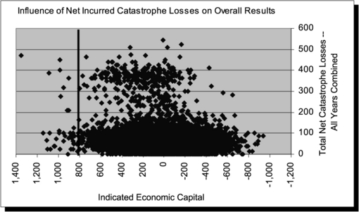
Often, the DFA model will confirm management’s expectations. However, sometimes the DFA model will present results that run counter to management’s intuition. In these situations, an added value of the model is realized—when unforeseen risks become apparent.
3.5.2 Example 2—Enterprise diversification benefit
The DFA system can also facilitate the exploration of the diversification benefit of a multi-line, multi-country insurance enterprise. This example shows the results of an analysis performed for a large multinational, multi-line insurance company. The company wanted to quantify the benefit from being diversified across multiple insurance lines with operations in different countries. The analysis began by dividing the enterprise into two business segments—life and property/casualty. The business segments were further divided by insurance line and by country of operation. Each line in each country then produced a DFA model using a set of consistent economic scenarios and the model results were combined. Figure 12 shows the required economic capital for the combined enterprise. The left-hand bar shows the amount of economic capital required when the enterprise is viewed as the sum of all the components. The middle bar shows the amount of economic capital required when the model results are aggregated at the business level. This allows for quantification of the diversification benefit attributable to multiple lines of business operating in multiple countries. The right-hand bar shows the required economic capital when the model results are aggregated at the enterprise level. This allows for the quantification of the diversification benefit attributable to the life and property/casualty business segments.

As a result of this analysis, the enterprise was able to quantify the benefit from operating multiple lines of business across multiple countries. At the present, this benefit is being held at the enterprise level rather than being distributed back down to the various business segments. Naturally, different enterprises may choose to distribute the benefit differently, depending upon their objectives. More is said about this issue in Section 4.
3.5.3 Example 3—Asset allocation
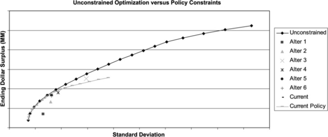
Studies have shown that asset allocation explains about 94% of the variability in portfolio returns (Brinson, Hood and Beebower, 1986). Hence, asset allocation policy is an important determinant that affects the financial health of the organization. In this next example we show how the DFA system can be used to aid in making asset allocation decisions. We begin by optimizing using the approach described in Section 2. Risk and reward can be defined in a number of ways. Reward is usually expressed as a desirable financial outcome. Risk is usually expressed as a function of the various performance indicators, although multiple indicators can define it. At its simplest, risk is equal to the standard deviation of the reward or as a target semi-deviation measure (i.e., downside risk below a specified return value—profit or surplus). In this example, we specify reward as ending surplus, and risk as the standard deviation of ending surplus.
Perhaps the most relevant report for assessing asset allocation is an efficient frontier. Figure 13 presents an example of an asset/liability efficient frontier, where the reward axis (y-axis) shows the expected surplus and the risk axis (x-axis) shows the volatility of surplus. Current and alternative policies can be shown together on the efficient frontier to demonstrate the risk/reward characteristics of each. A floating bar graph allows us to examine the percentile distribution of various alternatives. Figure 14 depicts a floating bar graph of the efficient asset mixes, current mix and alternative mixes.

These three examples and the preceding ones show the benefits of an integrated approach to evaluation and decision-making. The impact of any major decision can be evaluated on the entire organization. The value of each activity can be ascertained with regard to its benefit as a standalone business or as part of a portfolio of insurance products and services. The next section takes up these issues in more detail.
4 Capital allocation and decentralized risk management
The goal of a large multinational insurance company is to maximize its shareholder value, by means of growing the stock price with minimum volatility, by increasing the company’s economic surplus and by improving related performance measures. Operational inefficiencies may arise if a central committee must approve major decisions. Large financial companies operate on a global basis; it seems unlikely that a centralized decision making structure to be workable in a worldwide setting. (See Stein (2002) for a discussion of alternative organizational structures.) Thus, we turn to methods for improving a large organization by means of decentralized processes. A standard approach in risk finance is to allocate the firm’s capital to divisions or business units.6 Here, each unit operates as a standalone basis (at least in form) with its profits shown as a proportion of the company’s capital allocation.
As before, we assume that the corporate entity has been separated into distinct business units. There is much generality to this structure; for example, a unit can represent a new activity such as adding a new service to its businesses—selling life insurance in addition to auto insurance. This activity might be deemed a project, but for our purposes it is called a business unit. A unit can be the designated corporation within a country, aligned with regulatory oversight and accounting requirements. A large multinational financial company will often possess a relatively large number of units (divisions), depending upon the organizational set up and the regulatory constraints. The capital allocation constraint is as follows:
where the assigned capital for business unit k is ![]() and the total corporate capital is equal to the variable C within the DFA model.
and the total corporate capital is equal to the variable C within the DFA model.
For the first two subsections, we assume that headquarters can bring together the basic information for the corporation from each of the business units and can run a full DFA system. We relax this assumption in Section 4.3.
4.1 Bottom up capital allocation
Capital allocation can be carried out in two basic ways. First, a bottom up analysis can be performed as shown in Figure 15. Here each unit is evaluated in turn, considering the various risk metrics and the associated amount of required capital. In order to insure consistency, each unit should employ the same set of scenarios and probabilities, coming out of the scenario-generating module. By employing this approach, we develop a DFA model for business unit k so that the optimal decisions are made with reference to the situation of the unit on a standalone basis. In this context, the level of capital is an endogenous variable within the DFA model for each business unit. We assume that the unit will maximize a VM utility function or equivalent risk/reward function.

The capital for each unit is equal to ![]() for division k. The total required capital for the enterprise is then the sum of the required amounts—
for division k. The total required capital for the enterprise is then the sum of the required amounts—![]() .
.
There are several advantages. It fits traditional regulatory procedures since it aligns with standard processes. Local decision makers who are able to address local concerns can readily manage the procedure. Compensation can be linked to the outcomes of the divisions, without the need for any intervention from corporate headquarters. Implementation is relatively straightforward once the scenario generator is made available for each unit.
As a disadvantage, the capital allocation may lead to inefficient operations by requiring excess capital. The method may underestimate diversification benefits or ignore concentration exposures since it is difficult to coordinate the capital requirements across units. As a variant, capital allocation can be made using expert opinion regarding the business prospects and other aspects of the kth division. Given the specified capital, the division operates in a way to maximize its value. The corresponding decision variables are rendered by means of the local DFA system.
The final step of the top–down approach is to assemble the various plans for the business units into a single DFA system. Under the combined plan, the decision variables are fixed as determined previously. Information flows from the business units up to the headquarters. At this point, the company’s capital requirements can be calculated based on the enterprise risk-reward measures. Depending upon the risk measure, the overall company will typically find that there are at least some diversification benefits for operating a multi-product or geographically separated company. These benefits can be transferred back to the business units or they might be held at the headquarters for use in future mergers or acquisitions. As a technical point, certain risk measures such as the standard Value-at-Risk will not always lead to lower capital requirements due to concentration of risks. Subadditive risk measures (Artzner et al., 1999) will avoid this problem. However, these measures may be too conservative, requiring excess capital for the overall enterprise. The top–down strategy, proposed next, avoids this potential pitfall.
The bottom up approach has been implemented in one of the largest global insurance companies. The DFA models were developed and implemented for 15 business units, operating in 8 countries, 7 Life units and 8 P/C units. Typically, the models incorporated 90+% of the business in each unit. In addition, client teams in each unit were trained in the economic capital approach, and built their DFA model. Each entity presented its results to a central management group, with the overall results presented to client’s board of director. In this context, the bottom up approach has shown itself to be a practical procedure.
A few comments are relevant regarding this implementation. First, the different types of business require markedly different levels of economic capital (Figure 16). These differences are sometimes greater than conventional wisdom or rules of thumb would advise. Also, the differences from regulatory requirements are also marked—and slice in both directions. In some business segments the economic capital requirements are entirely met by margins in reserves, whereas in other business units the DFA strategies materially affect capital requirements. The economic capital assists in the measurement of the value of the units and forms the basis for performance evaluation measures (Figure 17). A potential disadvantage of the approach is the need to re-run the DFA system when significant changes in the corporation occur.


4.2 Top–down capital allocation
Under this approach, the firm’s capital is determined by means of the integrated risk management system at the headquarter level, aimed at modeling the entire organization. The resulting DFA system is run for the entire organization at a relatively detailed level. Then, given these results that include diversification benefits and concentration penalties, the projected capital allocation values for each division are computed and communicated to the division heads. See Figure 18 for a flow chart of the resulting information flows.
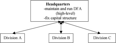
Fig. 18 Top–down capital allocation. (Information flows down from headquarters to divisions, e.g., capital allotments, with divisions supplying projected performance measures based on headquarters allocations and/or prices.)
Running the DFA system at headquarters accomplishes several aims. First, the required capital for the enterprise is calculated as a single entity. The decision variables can be set so that diversification benefits are optimizing along with expected profits and risk measures. In addition, the projections of rare events can be done without assuming a multivariate normal distribution for losses. The enterprise is optimized in systematic fashion, based on the best global information.
Unfortunately, several difficulties may arise when a centralized DFA system is run in a large multinational insurance company. Mostly, the information required and the organizational support structure is often inadequate at headquarters. There are simply too many constraints and relationships needed to find the optimal strategies for the business units. Also, the units can be hesitant to follow the dictates of a central administrator. As a consequence, the top–down approach, while theoretically attractive, poses a number of implementation barriers. The next section takes up the topic of finding a practical approach.
4.3 Decentralized DFA
This section takes up the issue of managing a company within a decentralized setting. Rather than assuming that headquarters reviews the major decisions, we desire to evaluate decisions on an ongoing basis without running the DFA system. The proposed approach is based on a well-formulated theory in optimization—called large-scale optimization (see Lasdon (1970) for an early reference). The goal is to combine the best of the top–down and the bottom-up approaches, by sending information between headquarters and the business units in a systematic fashion. To develop the approach, we first define the standard valuation formula for evaluating new activities, using risk adjusted discounting. We call this a static evaluation formula:
Static valuation.
where the cashflows (both positive and negative) are defined for division j at time t as ![]() , and where the discount factor
, and where the discount factor ![]() depends upon the calculated risks for division j (called the risk adjusted discount factor).
depends upon the calculated risks for division j (called the risk adjusted discount factor).
Next, we show that this standard valuation calculation can be expanded to address the marginal benefits (if any) when evaluating new projects/activities (see below). Beforehand, we extend the static evaluation to consider the cost of capital within the valuation formula:
Risk-adjusted profit (relative version)
where the profit for division j at time t is ![]() , and its capital is
, and its capital is ![]() and where the risk adjusted profit for division j is
and where the risk adjusted profit for division j is ![]() .
.
There is a large body of literature on the calculation of risk-adjusted returns on capital, largely coming out of banking applications. See Doherty (2000), Matten (1996), Shimpi et al. (2000), Zaik, Walter and Kelling (1996). An alternative to the ROP formula is one that charges the units an amount based on the capital allocation and the risk engaged in:
Risk-adjusted profit (value added version)
where the profit for division j is adjusted by subtracting its cost of capital, ![]() .
.
The value added approach provides an alternative to the relative calculation; these concepts are known as Economic Valued Added (EVA) and promoted by firms such as Stern Stewart (Ferguson, and Leistikow, 1998; Uyemura, Kantor and Pettit, 1996).
Capital allocation decisions have a substantial impact on relative profitability and “value” for each division and as a consequence there is controversy regarding calculating capital allocation. Importantly, everyone agrees that the amount of capital should depend upon the risks inherent in the division; activities possessing high risks must be backed with more capital as compared with other activities. However, current methods do not employ the DFA framework, grounded in a dynamic optimization context. See Froot and Stein (1998), Mulvey, Correnti and Lummis (1997), and Mulvey, Simsek and Pauling (2003) for discussions of optimizing a financial intermediary.
As an alternative, we can manage an insurance company by means of a decentralized DFA approach. The ideas build on the literature on large-scale optimization. Under this theory, a single optimization problem is broken into a set of smaller, more manageable subproblems, to be solved in a sequential fashion with coordination from a headquarters. Figure 19 shows the process. Note the similarity with the goals of capital allocation. Information is sent to the divisions, typically prices of joint resources under each of the scenarios—the state prices. In turn, the divisions optimize their affairs given these prices.
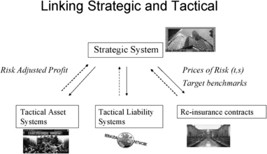
4.3.1 Corporate objectives in a decentralized setting
There are several goals for capital allocation to business units:
These goals must be part of any decentralized DFA system. An integrated planning system requires a systematic objective function in order to search for a set of recommendations for improving the organization. This issue can become complicated when local requirements and constraints exist for individual entities. A global insurance company operates within a large number of regulatory boundaries, including countries, states, cities, and other geographical regions, as well as offering a wide range of products (each with its own rules, traditions, etc.).
Generally, the objective of a business unit is to maximize shareholder value—as measured by the long-term growth of the company’s stock (and/or surplus). There may be few commonly agreed definitions of this growth on an anticipatory basis for a business unit, since units may not be trades in a market. Still, the risk-adjusted profits as developed above can serve to define the unit’s objectives.
4.3.2 Constraining the feasible region
Regulatory issues can be addressed by means of additional constraints on the integrated system. For instance, there are often accounting and statutory rules to be followed in order for the entity to continue to operate within its existing territories. These rules are often complicated due to the continual evolution of regulations in the financial industry. In addition, the divisions may have constraints imposed by the headquarters, such as the type and location of business it can engage in.
4.3.3 Decentralized DFA algorithm
The DFA system provides an ideal framework for analyzing the benefits of undertaking new activities and for changing the level of an existing activity. For instance, we can extend the static valuation calculation by employing scenarios and a scenario dependent discount factor. The result is a
Dynamic valuation formula
The risk adjusted discount factors ![]() are derived from the DFA system as dual variables for the joint capacity constraints (Eqs. (2) and (3)). These dual variables approximate the Arrow–Debreu state prices. A new activity can be evaluated on the margin as to its benefit or penalty to the organization. Diversification aspects are addressed in a direct fashion.
are derived from the DFA system as dual variables for the joint capacity constraints (Eqs. (2) and (3)). These dual variables approximate the Arrow–Debreu state prices. A new activity can be evaluated on the margin as to its benefit or penalty to the organization. Diversification aspects are addressed in a direct fashion.
For decisions with large impacts, the headquarters model must be rerun to evaluate the contribution of the decision. A marginal analysis is inadequate due to the changing nature of the state prices for substantial changes in the organization’s position. This result comes directly from linear programming theory.
In a similar fashion, we can employ the state prices for calculating risk-adjusted profits:
 (15)
(15)Again, these calculations more accurately reflect the impact of the divisional decision on the total firm than the simple formula presented earlier.
The full-decentralized DFA system employs a series of iterations—between headquarters and the business units. At each step, the headquarters takes in the solutions of the divisional DFA results in a manner similar to the bottom-up approach. Headquarters will then solve its own DFA system in order to determine the total capital for the organization. In this context, the optimal reinsurance treaties will be calculated. A new set of state prices (dual variables as state prices) for each scenario ![]() will emerge from this step and be transmitted back to the divisions. The decentralized DFA system combines elements of both the top–down and the bottom-up strategies. The business units optimize their affairs, given state prices for the scenarios. Headquarters optimizes its decisions by combining the decisions proposed by the business units; it determines the optimal capital structure, the shape of reinsurance treaties and other firm-wide issues. Periodically, a new set of state prices will be issued to the units for their decision-making. The approach is an extension and adaptation of the Dantzig–Wolfe decomposition method, with modifications for the stochastic nature of the DFA problem and the fact that headquarters will render decisions as discussed. In addition, the Dantzig–Wolfe method requires that headquarters finds the best convex combination of all decision proposals; this requirement would be difficult to implement in practice.
will emerge from this step and be transmitted back to the divisions. The decentralized DFA system combines elements of both the top–down and the bottom-up strategies. The business units optimize their affairs, given state prices for the scenarios. Headquarters optimizes its decisions by combining the decisions proposed by the business units; it determines the optimal capital structure, the shape of reinsurance treaties and other firm-wide issues. Periodically, a new set of state prices will be issued to the units for their decision-making. The approach is an extension and adaptation of the Dantzig–Wolfe decomposition method, with modifications for the stochastic nature of the DFA problem and the fact that headquarters will render decisions as discussed. In addition, the Dantzig–Wolfe method requires that headquarters finds the best convex combination of all decision proposals; this requirement would be difficult to implement in practice.
Also, from a practical standpoint, the number of iterations should be relatively few to reduce the costs and time to carry out the procedure. The state prices should not change in a radical way between iterations, if possible. The nature of the optimization should take into account these issues by adding constraints and/or penalties to the dual variables in the DFA system. A presentation of decentralized DFA appears in Erkan (2006), and Mulvey and Erkan (2006).
In summary, decentralized DFA provides a practical framework for managing the risks of a large organization while improving the firm’s profitability. A company that understands its risks can decrease overall risks and increase profits—at the same time. The decentralized organizational structure can be preserved so that individual can operate in a semi-autonomous fashion and more importantly can respond to the strict regulatory constraints and operating procedures.
5 Conclusions and future work
This paper describes the modeling of insurance companies within the enterprise framework. We present several prominent decisions, including asset allocation, evaluating new business activities, and other areas in which DFA improve long-run performance. A prominent example involves the optimal design of reinsurance treaties; a firm’s performance is directly affected by these agreements. In addition, we describe capital allocation issues from the standpoint of managing a large global company. The overriding goal is to optimize the enterprise value in a decentralized fashion.
We focus on significant issues that arise when constructing, simulating and ultimately optimizing a DFA system. We discuss convergent risks and the related matter of capital allocation based on risk measures affected by the tails of the profit/loss distributions. Not only must we estimate the expected loss payouts and other cash flows, but also we must determine the co-movements of these values, especially during periods of moderate to extreme volatility. The firm’s capital allocation decision is critical: capital protects the organization from credit downgrades and even bankruptcy. A nonlinear factor model provides the best approach, in our opinion, for modeling uncertainties. The DFA system helps develop the company’s responses to stressful scenarios in an anticipatory fashion. Optimization can play a significant role by pinpointing the best responses to the difficult scenarios, as well as balancing these responses when favorable scenarios occur.
What are barriers to wider implementation, similar to the success of enterprise management systems common in logistics and the process industry? First, the regulatory bodies, rating agencies, and company executives will need to become familiar with the advantages and disadvantages of the approach. Second, DFA promises to improve the profitability of a company while decreasing enterprise risks. As leading companies fulfill this promise, others will follow. It took considerable time before supply management became the norm in the process industry, even though examples were evident for many years beforehand. Also, regulation in the financial industry will have a direct impact on the use of DFA models. As an example, banking regulations have largely driven the development of risk management systems for banks vis-à-vis the Basel accords.
There are several directions for future research. First, study is needed of the processes causing the tails of the profit/loss distribution, especially factors that give rise to contagion. As an example, some hedge funds employ convergent trades based on differential amounts of liquidity. For these trades, there should be a factor in the hedge-fund risk model relating to liquidity and credit risks. Insurance companies work hard to minimize adverse selection and correlated losses. Still, improved risk transfer mechanisms will provide better liquidity and enhance information.
As novel insurance/financial products and services become available, the regulatory framework should be aimed at improving the industry’s risk-reward profile. It is in the best interest of the public to reduce the overall risks to insurance organizations. In the US, state regulators will be ultimately held responsible for losses that fall outside the company’s capital position. There are many mechanisms for reducing the company’s risks, including reinsurance, securitization, selective underwriting, and greater levels of capital. Each alternative can be tested via the DFA system to determine their respective costs and benefits. There may be companies who will try to understate their low probability, high-severity risks, and this coupled with the asymmetric information leads to interesting game theoretical issues. Just as in bidding, however, governmental regulators should strive to find solutions that are in the long-term interest of the parties. Aligning these interests will be an important topic for future research.
Last, financial companies will continue to merge diverse operations, such as insurance, banking, and security firms. Managing these financial conglomerates will require not only new managerial skills but also risk management systems that link together capital across diverse areas. Decentralized approaches will be needed for coordinating large global organizations.
Appendix A Toolkit for constructing a DFA system
This appendix describes the use of software tools for constructing a DFA system. As evident, a DFA system can become complex since it must include a large number of interacting variables, data sources, and processes. Simplifying the construction of a DFA system provides several benefits. First, a well-conceived toolkit can reduce the cost of development. Building a C++ system can take several years and cost over $1 million just for the software developers! The computer developer costs can be much reduced by employing a toolkit.
Second and importantly, the developer’s toolkit provides a blueprint for the construction of the DFA system. The assumptions are readily shown by reference to the construction diagrams, as evident in the figures listed in this appendix. Each of the modeling assumptions and the choices are apparent. Accessibility has several purposes. First, the DFA model can be easily changed as new information is collected or as mergers and acquisitions modify the organization. The DFA system has the ability to anticipate possible changes as well, for example, the impact of adding a new line of insurance can be evaluated. Thus, sensitivity analysis can be directly performed without the need for costly rewriting the DFA system.
Figure 20 provides the main elements of a sophisticated DFA toolkit. The heading—economic scenarios, investment operations, insurance operations, non-insurance operations, and corporate and financing operations—identify each aspect of the model. Likewise, a number of example models are depicted, such as alternative asset allocation strategies. These can be compared with each other across multiple dimensions. The goal of the software toolkit is to manage a set of DFA models for a large, complex organization. Simplicity and ease of access are the primary subgoals.

For each of the main sections, we can drill down to the special requirements for that topic. As an example, we define the economic scenarios in two ways—as deterministic time series values or as a group of stochastic scenarios. Figure 21 gives an idea of the former. Herein, a single scenario is chosen for an analysis. Economic scenarios fall into three classes—underlying economic factors, asset classes, and yield curves. The basic data is stored in files for ready access.

The same notions apply to the generation of the business lines as shown in Figure 22. There are many interacting issues in constructing the projected losses for each insurance line. Again, the goal is to build up from previously stored generic patterns. The figure involves the development of commercial automobile insurance, in this example, the expense patterns for the next six years. Commissions and other variable expenses are defined as a function of the time in the future. We fix these values as shown. Other issues, such as reserving and the loss patterns are defined in a similar fashion. The DFA modeling exercise begins at the highest level and works it way down to the specific elements for the business lines.

A second insurance product is depicted in Figure 23. Here, we define the cumulative loss payments for homeowner insurance—70.32% of the losses on average occur during the first year, 93.11% by the end of the second year, 97.63% by the end of the third year, and 100% by the end of the fourth year. This pattern is one of many possibilities, depending upon the types of products available to the insurance company. Each business activity is defined in turn.

A significant application of DFA involves the definition of reinsurance treaties. Each contract must be carefully constructed by reference to the primary losses and the resulting impact on the overall losses. Figure 24 depicts a reinsurance example with aggregate stop losses. The main forms of Reinsurance are saved for future analyses.

Last, we build the dividend policy for the company in Figure 25. In this case, the dividends can be positive or negative depending upon the target surplus. If a deficit occurs under this regime, there will be a capital infusion. Otherwise, a dividend will be made to the stockholders or the policyholders. The dividends flow from these assumptions.

While there are many other aspects, it should be evident that the toolkit approach greatly simplifies the construction of the DFA model. The assumptions are clearly delineated and easily found by the insurance users and DFA developers. Implementation of complex mathematical models is greatly improved and made more efficient by these software tools.
* Research support from the US National Science Foundation (DMI 0323410) and Towers Perrin and its Tillinghast subsidiary are gratefully acknowledged.
References
P. Artzner, F. Delbaen, J.M. Eber, D. Heath. Coherent measures of risk. Mathematical Finance. 9, 1999.
Berger, A., Madsen, C., 1999. A comprehensive system for selecting and evaluating DFA model parameters, in: Casualty Actuarial Society Forum, Summer
Berger, A., Mulvey, J.M., Nish, K., 1998. A portfolio management system for catastrophe property liabilities. in: Casualty Actuarial Society Forum, pp. 1–14
J.R. Birge, F. Louveaux. Introduction to Stochastic Programming. New York: Springer-Verlag; 1997.
G.C.E. Boender. A hybrid simulation/optimization scenario model for asset/liability management. European Journal of Operations Research. 99, 1997.
B. Bowers. Ready for anything. Best’s Review. 2002. February
G. Brinson, R. Hood, G. Beebower. Determinants of portfolio performance. Financial Analysts Journal. 1986. July–August
Burket, J., McIntyre, T., Sonlin, S., 2001. Dynamic financial analysis: DFA insurance company case study. in: Casualty Actuarial Society Forum, Spring
D.R. Cariño, W.T. Ziemba. Formulation of the Russell–Yasuda Kasai financial planning model. Operations Research. 1998. July–August
T.K. Cariño, D. Myers, C. Stacy, M. Sylvanus, A. Turner, K. Watanabe, W. Ziemba. The Russell–Yasuda Kasai model: An asset liability model for a Japanese insurance company using multi-stage stochastic programming. Interfaces. 1994;24:29-49.
Chen, Z., Bakshi, G., 2001. Stock valuation in dynamic economics. Yale University Report, ICF working paper, May 29
G. Consigli, M. Dempster. The CALM stochastic programming model for dynamic asset–liability management. In: W.T. Ziemba, J.M. Mulvey, editors. Worldwide Asset and Liability Modeling. Cambridge University Press, 1998.
A. Consiglio, S. Zenios. Integrated simulation and optimization models for tracking international fixed income indices. Mathematical Programming. 2001;89(2):311-339.
G. Dantzig, G. Infanger. Multi-stage stochastic linear programs for portfolio optimization. Annals of Operations Research. 1993;45:59-76.
Dert, C.L., 1995. Asset liability management for pension plans, PhD thesis. Erasmus University, Rotterdam
N. Doherty. Integrated Risk Management: Techniques and Strategies for Managing Corporate Risk. McGraw-Hill; 2000. March
D. Duffie, K. Singleton. Simulated moment estimation of Markov models of asset prices. Econometrica. 1993;61:929-952.
R. Enz, K. Karl. Profitability of the non-life insurance industry: its back-to-basics time. Swiss Re Sigma. 5, 2001.
Erkan, H.G., 2006. Decentralized enterprise risk management for global companies. PhD thesis. Princeton University, NJ
R. Ferguson, D. Leistikow. Search for the best financial performance measures: basics are better. Financial Analysts Journal. 1998. January–February
R. Fernholz, B. Shay. Stochastic portfolio theory and stock market equilibrium. Journal of Finance. 1982;37:615-624.
K. Frauendorfer, M. Schurle. Stochastic optimization in asset and liability management: a model for non-maturing accounts. In: S. Uryasev, editor. Probabilistic Constrained Optimization: Methodology and Applications. Kluwer, 2000.
K. Froot, J. Stein. Risk management, capital budgeting and capital structure policy for financial institutions: an integrated approach. Journal of Financial Economics. 1998;47:55-82. January
A. Geoffrion, R. Krishnan. Prospects for operations research in the e-business era. Interfaces. 2001;31:6-36. March
C. Gourieroux, A. Monfort, E. Renault. Indirect inference. Journal of Applied Econometrics. 8, 1993.
Hoyland, K., 1998. Asset liability management for a life insurance company: a stochastic programming approach. PhD Dissertation. Norwegian University of Science and Technology
K. Hoyland, S. Wallace. Generating scenario trees for multistage problems. Management Science. 2001:295-307. February
Kaufman, A., Ryan, T., 2000. Strategic asset allocation for multi-line insurers using dynamic financial analysis. in: Casualty Actuarial Society Forum, Summer
M.I. Kusy, W.T. Ziemba. A bank asset and liability management model. Operations Research. 1986;34:356-376.
L. Lasdon. Optimization Theory for Large Scale Systems. London: Macmillan; 1970.
D. Laster, E. Thorlacius. Asset-liability management for insurers. Swiss Re Sigma. 6, 2000.
G. Lin, M. Ettl, S. Buckley, S. Bagchi, D. Yao, B. Naccarato, R. Allan, K. Kim, L. Loenig. Extended enterprise supply chain management at IBM Personal Systems Group and other divisions. Interfaces. 30, 2000. January–February
Lowe, S.P., Stanard, J., 1996. An integrated dynamic financial analysis and decision support system for a property catastrophe reinsurer. In: CAS Seminar on Dynamic Financial Analysis, Spring CAS Forum
Mango, D., Mulvey, J.M., 2000. Capital adequacy and allocation using dynamic financial analysis. In: Casualty Actuarial Society Forum, Summer
C. Maranas, I. Androulakis, A. Berger, C.A. Floudas, J.M. Mulvey. Solving stochastic control problems in finance via global optimization. J. Econ. Dyn. Control. 1997;21:1405-1425.
C. Matten. Managing Bank Capital: Capital Allocation and Performance Measurement. John Wiley; 1996.
J.M. Mulvey. A surplus optimization perspective. Investment Management Review. 3, 1989.
J.M. Mulvey. Generating scenarios for the Towers Perrin investment system. Interfaces. 26, 1996.
Mulvey, J.M., Correnti, S., Lummis, J., 1997. Total integrated risk management: insurance elements. Princeton University Report SOR-97-2
J.M. Mulvey, H.G. Erkan. Applying CVaR for decentralized risk management of financial companies. Journal of Banking and Finance. 2006;30(2):627-644.
J.M. Mulvey, G. Gould, C. Morgan. An asset and liability management system for Towers Perrin–Tillinghast. Interfaces. 2000;30:96-114.
J.M. Mulvey, D. Rosenbaum, B. Shetty. Parameter estimation in stochastic scenario generation systems. European Journal of Operations Research. 1999;118:563-577.
Mulvey, J.M., Simsek, K., Pauling, W., 2003. A stochastic network approach for integrating pension and corporate financial planning. Innovations in Financial and Economic Networks
J.M. Mulvey, A. Thorlacius. The Towers Perrin global capital market scenario generation system: CAP:Link. In: W.T. Ziemba, J.M. Mulvey, editors. Worldwide Asset and Liability Modeling. Cambridge University Press, 1998.
J.M. Mulvey, C. Ural, Z. Zhang. Improving performance for long-term investors: wide diversification, leverage, and overlay strategies. Quantitative Finance. 2007;7(2):1-13.
A. Perold, W. Sharpe. Dynamic strategies for asset allocation. Financial Analysts Journal. 1988:16-27. January
R.T. Rockafellar, S. Uryasev. Optimization of conditional Value-At-Risk. The Journal of Risk. 2000;2(3):21-41.
R.T. Rockafellar, R.J.-B. Wets. Scenarios and policy aggregation in optimization under uncertainty. Mathematics of Operations Research. 1991;16:119-147.
R. Rush, J.M. Mulvey, J. Mitchell, T. Willemain. Stratified filtered sampling in stochastic optimization. J. Appl. Math. Decision Sci.. 2000;4:17-38.
P.A. Shimpi, C. Helbling, D. Durbin, D. Laster, editors. Integrating Corporate Risk Management. Texere, 2000. December
J. Stein. Information production and capital allocation: decentralized vs. hierarchical firms. J. of Finance. 2002. October
D. Uyemura, C. Kantor, J. Pettit. EVA for banks: value creation, risk management and profitability measurement. J. of Applied Corporate Finance. 9, 1996. Summer
A. Wilkie. Stochastic investment models: theory and applications. Insurance: Mathematics and Economics. 1987;6:65-83.
K. Worzel, C. Vassiadou-Zeniou, S.A. Zenios. Integrated simulation and optimization models for tracking fixed-income indices. Operations Research. 1995;42:223-233.
E. Zaik, J. Walter, G. Kelling. RAROC at Bank of America: from theory to practice. J. of Applied Corporate Finance. 9, 1996. Summer
S.A. Zenios. Massively parallel computations for financial planning under uncertainty. In: J.P. Mesirov, editor. Very Large Scale Computation in the 21st Century. Philadelphia: Society for Industrial and Applied Mathematics; 1991:273-294.
S.A. Zenios. Financial Optimization. Cambridge: Cambridge University Press; 1993.
S.A. Zenios. Asset and liability management under uncertainty for fixed income securities. In: W.T. Ziemba, J.M. Mulvey, editors. Worldwide Asset and Liability Modeling. Cambridge University Press, 1998.
W. Ziemba, J.M. Mulvey, editors. Worldwide Asset and Liability Modeling. Cambridge University Press, 1998.
1 Bill Pauling worked at Towers Perrin during the writing of this article.
2 Steve Britt worked at Towers Perrin during the writing of this article.
3 Dominated solutions have the usual interpretation—better objectives along one or more dimensions, while keeping all other dimensions at the same level of utility.
4 Dynamic stochastic control can be employed in certain simplified circumstances. See Ziemba and Mulvey (1998).
5 Strictly speaking, uncertainties can be modeled by means of continuous functions. However, a sampling scheme is needed to render the problem tractable. See Birge and Louveaux (1997) and Consigli and Dempster (1998) for discussions of scenario selection.
6 We allow all parts of the organization to be business units—including independent companies, etc.