
Handbook of Asset and Liability Management, Vol. 2, No. suppl (C) • 2007
ISSN: 1872-0978
doi: 10.1016/S1872-0978(06)02020-5
Chapter 20 Dynamic Asset and Liability Management for Swiss Pension Funds
Abstract
We present an asset and liability model for Swiss pension funds. This includes an asset dynamics model and an optimisation technique to solve the problem of allocating the funds considering the liabilities maturity structure. Our liability model is based on the current and projected future cash outflows of all members, taking into account: projection of the individuals’ income, probabilities of entry and exit of members, and probabilities of death and invalidity of members. For the modelling of the various probabilities, we use a life insurance mathematics approach. This results in a dynamic, stochastic description of the pension fund liabilities. The projected uncertain future cash flows are sorted by their date of payment. Payments in a certain period are summed up in liability buckets. Furthermore, we compute the obligations that arise from the current wealth of funds where future contributions are not taken into account. Similar to the liability buckets, the obligations are also summed up into obligation buckets. The buckets give a manageable description of the pension fund’s liabilities (and obligations) and their term structure. The assets are modelled from the perspective of a Swiss investor. We use a dynamic factor model with heavy tailed residuals to model stock and bond market prices. We propose an optimisation technique for the asset liability management problem where the liability buckets are matched with available wealth of the pension fund. The optimisation problem is to minimise the shortfall of bucket funding while reaching a required future surplus. The solution results in an asset allocation for each liability bucket based on its time horizon. In this way we realise the life-styling hypothesis for each individual across the entire pension fund. In a case study we apply this method to the data of a Swiss pension fund with over 3500 members and over 1 billion (109) Swiss Francs of wealth.
Keywords
• asset and liability management • life insurance model • asset and liability portfolio optimisation • factor models
JEL classification
• C61 • G11 • G23
1 Introduction
Pension funds manage a significant amount of wealth. It is therefore highly relevant that they manage their wealth in a responsible way while always taking into account their very long time horizon. Asset and liability management for pension funds has several different issues. There is the traditional asset management and portfolio optimisation with the appropriate asset price models. There are also models describing the pension funds liabilities which depend on the type of pension fund. The combination of asset management with the liabilities of a pension fund leads to a true asset liability management.
1.1 Pension fund liability modelling
An important aspect of pension fund liability modelling is the way in which the pension fund members incomes are modelled. The income is central, since it defines the contributions into the pension fund. Very generally, Merton models a deterministic wage income in the framework of dynamic portfolio optimisation with consumption (Merton, 1992, Part II). Boulier, Huang and Thaillard (2001) then provide a pension fund model in continuous time with deterministic salaries. Further, pension fund related papers, such as Battocchio and Menoncin (2004), Cairns, Blake and Dowd (2000) or Bodie et al. (2004) provide stochastic models for wages, modelled with one or more Brownian motions for salary changes due to interest rate changes and company stock price changes, among others. Our model for salaries is based on Cairns (2003), where salaries are increased in relation to a cost-of-living index and an age related function.
Pension-fund models have been used in simulation tools which take into account the mortalities of pension fund members and what this implies on the pension fund liabilities (Kingsland (1982); Winklevoss (1982); Bacinello (1988); Chang (1999); and Ziemba (2003, Chapter 4)). Motivated by an actuarial approach based on the mathematics used for life insurances as in Gerber (1997) or the technical summary given in connection with a Swiss life table EVK (2000) we also use mortality probabilities in our model. A different approach to modelling pension funds is given by Blake (1998), where pension fund schemes are modelled in a framework of financial options. A full book on modelling pension systems (Simonovits, 2003) covers many issues from life cycle, funded, and unfunded systems to issues of demographics and the transition of pension systems.
1.2 Asset and liability management optimisation for pension funds
Contribution rates are an important factor in pension fund management. Since the main interest of (young) pension fund members is mostly to pay small contributions and generate higher returns by investing a larger proportion in riskier assets (such as stocks) in the financial markets. Optimisation is based on a trade-off between contribution rate and the pension fund liquidity, resulting in an investment strategy (O’Brien (1986); Haberman and Sung (1994); Reichlin (2000); Taylor (2002); and Josa-Fombellida and Rincon-Zapatero (2004)). Further optimisation methods for pension fund investment strategies in continuous time are given in Cairns, Blake and Dowd (2000) and in Haberman and Vigna (2002) for defined contribution pension plans. Optimal investment strategies for special cases of pension funds, such as minimum guarantees or pension fund accumulation and decumulation, are solved with CRRA utility functions in continuous time in Deelstra, Grasselli and Koehl (2003) and in Battocchio, Menoncin and Scaillet (2003), respectively. Furthermore, Devolder, Bosch-Princep and Fabian (2003) and Charupat and Milevsky (2002) describe stochastic optimal control solutions for optimal asset allocation for life annuities. Another approach tries to capture the investment preferences of an individual investor whose investment horizon shortens with advancing age and to implement this behaviour into an investment strategy applicable to the total wealth of the pension fund. The asset allocation is a function of risk aversion and time horizon and has been described in Brennan, Schwartz and Lagnado (1997) and Campbell and Viceira (2002) for the individual and also in Cairns, Blake and Dowd (2003), called stochastic life-styling, as a strategy for pensions saving.
Common risk measures used in asset and liability management situations are Value-at-Risk (VaR) and Conditional Value-at-Risk (CVaR). Blake, Cairns and Dowd (2001) estimate the VaR with regard to pension plan design and Dowd, Blake and Cairns (2003) investigate long-term VaR. Further, CVaR has been applied to a pension fund in Bogentoft, Romeijn and Uryasev (2001) and Bosch-Príncep, Devolder and Domínguez-Fabián (2002). Several other studies considered asset liability management, although not in the context of pension fund management, they are very relevant and applicable for the specific case of the pension fund. Ziemba and Mulvey (1998), Ziemba (2003), Zenios (2002) authored books covering the broad field of asset and liability management, specially for long-term financial planning. Papers on long-term planning are Mulvey, Pauling and Madey (2003), Mulvey and Shetty (2004), Kusy and Ziemba (1986) and Cariño and Ziemba (1998). Further references on asset and liability management are also given in Section 8.
1.3 Pension funds in the Swiss pension system
We describe a model for the liabilities of a Swiss pension fund. To give a broad overview on the Swiss pension system, we first describe the function of the Swiss pension funds within the total pension system.
The Swiss old-age insurance system consists of three pillars. The first pillar is intended to secure existence, the second pillar is to retain the living standard, and the third consists of individual retirement savings. The first pillar, the state pension, is financed through a national pay-as-you-go pension system. The contributions are split up between employer and employee and they are a fixed percentage of earned wages (currently 8.4%). There is no limitation on contributions (even for above-average salaries). However, there is a minimum and a maximum pension amount which is paid. The actual pensions are adjusted yearly (e.g., for 2004, monthly pensions for individuals were minimum 1055 Swiss Francs (CHF) and maximum 2110 CHF).
The second pillar, occupational pension, is financed through an employer-specific, earnings-related, and fully funded pension fund. The pension system is designed such that the first and second pillar together approximately result in a pension of 60% of the last wages which, after taxes should make it possible to retain one’s living standard after retirement. The participation is mandatory as soon as a given minimal salary is earned (currently 25,320 CHF). Above a certain wage level (75,960 CHF), there are possibilities for a more flexible investment of the additional wealth summarised by a term called “above-mandatory”. Contributions towards the pension fund are split up between employer and employee and are a percentage of earned wages (between 7 and 18%, depending on pension fund).
Technically, the funds are legally independent institutions whose funds are not linked with the sponsoring company or any other institution. The sponsoring company decides on whether the pension fund is to be run as a defined benefit (DB) or defined contribution (DC) plan. For the “above-mandatory” savings, more choices can be made by the employee regarding investment strategy. There is a minimum guaranteed annual return on the accumulated wealth specified by law. This return remained unchanged at 4% from 1985 until 2002, in 2003 it was reduced to 3.25% and in 2004 to 2.25%. For the DC plan, the meaning of the minimum return is obvious. For the DB plans the guarantee on the benefits remained the same and the minimum guaranteed return remains merely an accounting issue. Pension funds may be run by autonomous institutions for one (large) company alone. Others may consist of several companies of whose employees are pooled into one single pension fund. Still others may consist of very few members and be run by an actuary. Finally, certain large insurance companies also offer their services to run pension funds. Depending on its structure, a pension fund may be run as a non-profit organisation, whereas, for instance, the insurance companies that offer to run a pension fund want to make a profit from that business.
In the pension plan, the employees are guaranteed pension benefits upon reaching a given retirement age. For receiving full benefits, certain conditions apply with regard to years of service. In the DC scheme, annual pensions (benefit payments) are calculated using a formula based on accumulated wealth at retirement and a predefined factor (currently 7.2% of final wealth is given as annual pension, as specified by law). The factor is based on calculations related to average life expectancy at retirement. In the DB plan, the employees are guaranteed a percentage of their last earned salary (typically around 60%).
In addition to the first and second pillar, the third pillar consists of privately paid, tax-privileged savings. This kind of pension is voluntary and is used as a means to supplement the mandatory pension or, for example, to enable early retirement.
We focus on the second pillar, the (occupational) pension funds.
1.4 Analysis of major issues at managing a fully funded pension fund
In a pension system where the young active members’ and the retired passive members’ wealth is managed as fully funded pension fund, several (and possibly opposing) interests need to be met. In addition, there are legal requirements, such as minimal return and quantitative diversification rules, as well as uncertainties due to investment strategies and to demographic trends. All parties involved in the pension fund have their own particular interests: the pensioners and the active members shortly before retirement are interested in a secure and stable pension which is best achieved by a low-risk, conservative investment strategy. The younger active members are interested in the highest possible returns in order to augment their future pensions. The sponsoring companies’ interests, finally, lie in minimising the need for paying supplemental funds due to under-coverage of the pension fund.
The task of the pension fund manager is to achieve the goals of all parties involved, while observing the legal requirements, achieving a minimal guaranteed return (in order not to become under-covered), and with the additional difficulties of uncertain market returns, liquidity needs and demographic trends.
In addition to the management problem with the opposing interests, Swiss pension funds used to re-distribute gains that were above the guaranteed minimal return. As reported in the press (e.g., in the Swiss newspaper “Neue Zürcher Zeitung” (NZZ, 2004)), a study that was done for a Swiss parliamentary commission found, that it is no longer possible to back-trace both the actual surpluses nor where these were distributed in the past. This surplus could either have been used to build reserves, have been re-distributed to the members, or used for (completely) other purposes that may have not benefited the pension fund members at all. The Swiss pension funds started to get into more and more trouble after the market downturn which started in the year 2000. Although academic models clearly indicated danger in the stock market in advance (Ziemba, 2003, Chapter 2), the general investment community did not expect the downturn after many years of constantly rising markets. As a consequence the pension funds reserves and investment strategies were often not up to their actual risk potential. Together with the guaranteed return which was fixed by a federal law, this led to the under-coverage of many pension fund. According to statistics and the press (e.g., NZZ (2004)), by the end of 2002 over 50% of pension funds were under-covered, i.e., their financial assets were not sufficient to cover their promised (expected) liabilities in the future. We could also observe that assets and liabilities were considered as separate entities leading to short-term liquidity management combined with an asset investment strategy that did not match the liabilities.
In the following sections we propose a solution to the problem of the opposing interests. We do this by analysing the pension funds population by means of life insurance mathematics, since we believe that a lot of information is contained in the structure of the pension fund members which can be exploited in order to find an investment and liquidity management strategy. Therefrom we can derive an asset and liability management strategy which should visibly tackle the interests of the involved parties. The solution not only yields an investment allocation strategy which takes into account the pension fund population structure, but may also be used as a means to fairly distribute possible surpluses and to still fulfil legal constraints.
1.5 Brief comparison of the Swiss and other pension fund systems
The following very brief comparison of international pension fund systems is taken from a larger comprehensive study of the OECD insurance and private pension compendium for emerging markets (OECD, 2001). We only discuss the second pillar or what is commonly organised under occupational pension. Every country we regarded has a very distinct and characteristic pension system. The pension systems mostly grew with the countries individual requirements and historical, economical and demographic issues. It is therefore hard to compare pension systems. We provide this overview for interested readers, who may wish to compare their own (and best known) pension system with the Swiss system.
Funding and risk bearing: Occupational pensions are an earnings-related fully funded system. Most funds are DC funds, whereas DB schemes are represented mainly in the public sector. There is a minimum nominal rate on the pensions savings (1985–2002: 4%, 2003: 3.5%, 2004: 2.25%). Excess returns must be re-distributed within the pension fund with a quota of at least 90% in the form of interruption of contribution payment (for active members and sponsoring companies), additional benefits (for pensioners) or reserves. The Administration of the pension funds can be done either by non-profit foundations, cooperative societies or as institutions incorporated under public law. Participation is mandatory for employees. The employers mandatorily decide on the pension fund for their employees. Contributions towards the pension fund are split between employee and employer, whereby the employer must at least pay 50%. Minimum diversification requirements apply: Investment in debt instruments of a single entity (except government bonds, banks, and insurance companies) is limited to 10% (5% for foreign assets). Investment in equity of a single company is limited to 10% (5% for foreign assets). Self-investment in the sponsoring company is limited to 10%. Investment in derivatives is allowable for hedging purposes only. There is an overall limit in investments in foreign bonds of 30%, of 25% in foreign equities and of 20% in foreign currency bonds. There are aggregate limits for domestic and foreign equity (50%), foreign bonds and foreign currency bonds (30%), as well as real estate and Swiss and foreign equity (70%). Supervision is effected by the federal office.
Funding and risk bearing: Occupational pensions may be made available as funded DB, hybrid or DC plans without any guarantees. They are administered by the sponsor (assets are managed in a closed pension fund by trustees), life insurance companies or as collective investment schemes (401(k)). Participation is voluntary. There are general requirements for diversification: For all DB plans and some DC plans: 10% limit on investment in employer securities or real property; no transactions with parties in interest (i.e., a fiduciary, provider of services, participant, plan sponsor, beneficiary, or some other party with a relationship to the plan). Assets must be under the jurisdiction of US courts.
Funding and risk bearing: IRAs are fully funded DB or DC schemes. IRAs invested in mutual funds or bank deposits offer no guarantees. IRAs invested in annuities offer their guarantees. They are administered either by a collective investment scheme provider, a bank or an insurance company (annuity). Participation is voluntary. There are general requirements for diversification: For all DB plans and some DC plans: 10% limit on investment in employer securities or real property; no transactions with parties in interest. Assets must be under the jurisdiction of US courts.
In contracted-out schemes members have their state pension (SERPS) rights included within their private scheme. Funding and risk bearing: They are funded DB or DC schemes. For DC plans, there is minimum mandatory annuisation (annuity must be bought at age 75). They are administered by trustees (via a closed pension fund) or a life insurance company. Participation is voluntary, but in case of an opt-out, they must sign up with an appropriate personal pension plan. There are general requirements for diversification and suitability. Employer related investment is limited to 5%. There are no quantitative portfolio restrictions.
In contracted-in schemes members have their state pension (SERPS) rights treated separately from their private scheme (private pensions benefits are paid in addition to SERPS). Funding and risk bearing: They are funded DB or DC schemes. Arrangements which may be unfunded to provide executives with extra retirement provision on earnings above the earnings cap. They are administered by trustees (via a closed pension fund) or a life insurance company. Participation is voluntary. There are general requirements for diversification and suitability. Employer related investment is limited to 5%. There are no quantitative portfolio restrictions.
Funding and risk bearing: The occupational pensions are funded and are mainly DB schemes. They are administered by a closed pension fund (foundation) or an insurance company. Participation for Employers is compulsory under collective bargaining arrangements and by statute in certain sectors. For employees participation is mandatory. Diversification is required but there are no quantitative rules.
2 Liability model for a Swiss pension fund
2.1 General assumptions
The pension fund’s liabilities consist of all current and future payments towards pensioners and insured active members. Pensioners receive a pension which is an annuity based on their income at retirement age or wealth accumulated by the time of retirement. Active members pay contributions during their working years in order to accumulate wealth for retirement age. Wealth is compounded with a minimal return. The rate of minimal return is specified by law. Active members may leave the pension fund, in which case the accumulated wealth must be transferred to their new pension fund. To get a detailed description of the pension funds payment streams we base our model on every payment to every pension fund member. This means that we regard the (remaining) expected payments to pensioners as well as projected expected outflows to today’s active members. In the calculation of liabilities we make several assumptions:
2.2 Pension fund liabilities and obligations
The pension fund’s liabilities can be modelled in two different ways, each having its later use in the asset and liability management optimisation. We differentiate between obligations and liabilities in the following way:
summarise the pension fund’s promised payments to pensioners and active members based on their current wealth. For obligations, we do not take into account any future contributions into the pension fund by active members. Pensioner’s obligations are the remaining pension benefit payments until death. For the active members, the obligations consist of the wealth accumulated at the moment which is compounded with the minimal return.
consist of the pension fund’s promised payments to pensioners and active members taking into account current wealth and including outstanding future contributions. Pensioners liabilities are the remaining pension benefit payments until death. For active members, we make assumptions on their projected future wages which leads to future contributions into the pension fund. When we project the future balance of the members’ accumulated wealth, we do not only compound with the guaranteed return, but future contributions are also included in the compounding process.
For pensioners there is no difference in obligations and liabilities. For obligations no assumptions are made on future wages and contribution payments. For liabilities these assumptions are used. Since contributions are not included and thus the wealth only accumulates with the (guaranteed) return, the obligations will always be smaller than the liabilities until the moment of retirement. By recalculating obligations every year (after contributions have been paid) we can update the past obligations calculation with the new obligations based on accumulated wealth plus new contributions. This way, the older the member gets, the difference between obligations and liabilities grows smaller and smaller. These characteristics of obligations and liabilities are described in the sections on modelling obligations and liabilities (Sections 4, 5, 6).
2.3 Pension fund bucket structure for asset management
We consider payments to every member individually. We thereby not only regard the amount, but also the instant at which the payment is due. This provides us with the expected payment stream over the regarded time horizon for every member in the pension fund. We further collect all payments due in a certain time period (e.g., one year) and call this the liability bucket for liabilities or obligations bucket for obligations. Liability payments due in the next year are then collected in the one-year liability bucket, payments due in two years in the two-year liability bucket, and payments due in j years are collected in the j-year liability bucket. The same can be done for obligations. This procedure results in the long-term structure of payments out of the pension fund. The bucket structure is then needed as an instrument for an advanced term-structure-oriented asset management.
3 Basic principles of the pension fund model
3.1 An actuarial perspective for pension funds
Not only do we regard guaranteed pension benefits and payment streams, but also the uncertainties that they are subjected to. Our model and the notation are influenced by the description used by actuaries in life insurance mathematics (e.g., as in Gerber (1997) and Koller (2000)). Apart from using survival probabilities and probabilities of becoming disabled, we need to know the probabilities for members leaving the pension fund before retirement, e.g., due to changing their employer, or leaving the country, summarised here by the term “labour mobility”. These figures have been derived in a study by Rufibach et al. (2001) based on data of the pension fund for the employees of all Swiss federal institutions.
All of the cases of uncertainty mentioned above have an influence on the pension fund payment streams. However, we cannot know whether or when they will occur. They can therefore be considered as risk factors of the pension fund. Since every individual member is assumed to be independent of the other, we can aggregate individual risks over the entire pension fund. The risk factors of the pension fund are highly dependent on the pension funds population and there are big differences between different population groups, young and old, or men and women, for instance. We will first go into the details of the different probabilities and then define a measure which gives us the total probability for a member to remain in the pension fund for a given number of years at a given age.
3.2 Death probability and probability of invalidity
Death probabilities are given in “life tables” consisting of the one-year death probabilities. They are built from statistical data which can be derived from a whole population or from a more specific, smaller group, such as pension fund members. When we consider a person aged α years, in year t we denote this by ![]() . The one-year death probability for this so-called “life aged
. The one-year death probability for this so-called “life aged ![]() ” is then
” is then ![]() . The one-year survival probability is given as
. The one-year survival probability is given as ![]() . Death probabilities for men and women differ mainly at high ages. We use the table (EVK, 2000) given by the Swiss pension fund for the Swiss federal employees based on its own statistics. This table is updated and published every ten years. The maximum age considered here is 105 years denoted by
. Death probabilities for men and women differ mainly at high ages. We use the table (EVK, 2000) given by the Swiss pension fund for the Swiss federal employees based on its own statistics. This table is updated and published every ten years. The maximum age considered here is 105 years denoted by ![]() . The survival probability over several years is
. The survival probability over several years is
 (1)
(1)which is the probability of a life aged α at time t to survive the next j years. The one-year invalidity probability ![]() for a life aged
for a life aged ![]() is the probability of a person becoming disabled within one year at a given age. The invalidity probability is given in tables similar to the known life tables until retirement age
is the probability of a person becoming disabled within one year at a given age. The invalidity probability is given in tables similar to the known life tables until retirement age ![]() (i.e., it is also contained in (EVK, 2000)). There is a much higher invalidity probability (almost with a factor of 2) for women below 50 than there is for men at the same age, whereas the invalidity probability for men rises rapidly for ages above 50.
(i.e., it is also contained in (EVK, 2000)). There is a much higher invalidity probability (almost with a factor of 2) for women below 50 than there is for men at the same age, whereas the invalidity probability for men rises rapidly for ages above 50.
3.3 Exit probability and entry rate
Exit probabilities depend strongly on the sample from which the statistical data is taken. We consider the one-year exit probabilities for a given age ![]() , denoted by
, denoted by ![]() , as found in (Rufibach et al., 2001) for the pension fund of the Swiss federal employees. The ages are restricted to 60 years for men and 57 for women since it is assumed that labour mobility can be disregarded within five years before retirement. The entry rate is defined as the number of new entries at a given age in relation to the actual number of members at the same age. For a given age
, as found in (Rufibach et al., 2001) for the pension fund of the Swiss federal employees. The ages are restricted to 60 years for men and 57 for women since it is assumed that labour mobility can be disregarded within five years before retirement. The entry rate is defined as the number of new entries at a given age in relation to the actual number of members at the same age. For a given age ![]() , we denote the entry rate by
, we denote the entry rate by ![]() . Here too, there is a big difference between men and women and different ages.
. Here too, there is a big difference between men and women and different ages.
3.4 Total exit probability
Active members face the risk of not surviving the next year, ![]() , risk of falling disabled,
, risk of falling disabled, ![]() and they may leave the pension fund (i.e., change employer), with probability
and they may leave the pension fund (i.e., change employer), with probability ![]() . From one year to the next, the age-dependent probability for an active member to stay in the pension fund is
. From one year to the next, the age-dependent probability for an active member to stay in the pension fund is
Then, ![]() is the one-year total exit probability for a member aged
is the one-year total exit probability for a member aged ![]() . This probability is shown in Figure 1 for men and women. The probability of an active member with age α at time t reaching an age
. This probability is shown in Figure 1 for men and women. The probability of an active member with age α at time t reaching an age ![]() in the future still being a member of the pension fund is
in the future still being a member of the pension fund is

 (3)
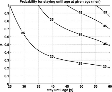
(3)With Eq. (3), we can find the probabilities of staying a number of years in the pension fund for every age ![]() . Figure 2 shows the curves generated for men of four different ages (25, 35, 45, and 55 years). As an example, we can find here that the probability for a man 25 years old to stay with the pension fund until 35 is approximately 0.43. To stay until pension, the probability for a 25-year-old is at 20%. Similar curves can be calculated for women. These probabilities depend on the sample and very different figures might appear for another set of statistical data of another pension fund.
. Figure 2 shows the curves generated for men of four different ages (25, 35, 45, and 55 years). As an example, we can find here that the probability for a man 25 years old to stay with the pension fund until 35 is approximately 0.43. To stay until pension, the probability for a 25-year-old is at 20%. Similar curves can be calculated for women. These probabilities depend on the sample and very different figures might appear for another set of statistical data of another pension fund.
3.5 Earnings projections
3.5.1 Projected wealth and salary
To project future pensions, we need to know final expected salaries or accumulated wealth at retirement (depending on the type of pension fund). Salaries may rise due to a multiplicative age-related factor (as described in Cairns (1994)), denoted by ![]() and similarly, a multiplicative cost-of-living related factor denoted by
and similarly, a multiplicative cost-of-living related factor denoted by ![]() , respectively. Let
, respectively. Let ![]() be the projected salary based on this year’s salary. Next year’s expected salary is
be the projected salary based on this year’s salary. Next year’s expected salary is
Salaries for ![]() are projected by
are projected by
Factors for salary rises are given as follows:
Salaries rise as a function of age due to work experience or career advances and also as a function of the current salary level. On average, higher salaries have greater increases than smaller ones and salary rises are larger for younger employees. The age-related effect may also become negative as employees get older. For a more detailed description of the effect, also with a differentiation between sex, education, and management levels, see Dondi (2003). The effects of earnings over a lifetime, also summarised under “life-cycle model”, are also described in Campbell and Viceira (2002), Clark et al. (2004), and Simonovits (2003). Detailed country studies of salary distributions are in Pittau and Zelli (2002) for Italy and for Brazil in Cowell, Ferreira and Litchfield (1998), respectively.
Cost-of-living-related increases reflect the effect of inflation on salaries. Here, we model the instantaneous rise in cost of living with the relative change of the consumer price index, denoted by ![]() , with a first-order autoregressive process (AR(1)),
, with a first-order autoregressive process (AR(1)),
with factor loading parameter A, constant b, variance parameter ν, and with the Gaussian white noise ![]() . As factor, we use the Swiss consumer price index (CPI). The parameters are estimated using ordinary least square, as described in Hamilton (1994).
. As factor, we use the Swiss consumer price index (CPI). The parameters are estimated using ordinary least square, as described in Hamilton (1994).
For obligations, the projected wealth in j years ![]() is obtained just by compounding the actual wealth with the guaranteed return
is obtained just by compounding the actual wealth with the guaranteed return
To calculate the liabilities projected wealth in j years ![]() , the active member’s wealth is accumulated by adding up regular payments and investing the already saved wealth at the guaranteed interest
, the active member’s wealth is accumulated by adding up regular payments and investing the already saved wealth at the guaranteed interest ![]() . Contribution payments consist of an (age-dependent) fraction
. Contribution payments consist of an (age-dependent) fraction ![]() of the salary
of the salary ![]() . The projected wealth is
. The projected wealth is
 (7)
(7)which is the current wealth compounded with ![]() , the guaranteed return, plus the sum of all projected contribution payments over the next j years. The latter are also compounded with
, the guaranteed return, plus the sum of all projected contribution payments over the next j years. The latter are also compounded with ![]() for every year after they have been paid into the fund. Define the projected wealth accumulated at retirement age
for every year after they have been paid into the fund. Define the projected wealth accumulated at retirement age ![]() as
as ![]() for obligations and
for obligations and ![]() for liabilities. The final salary at retirement age is
for liabilities. The final salary at retirement age is ![]() .
.
3.6 Pension fund plans
For the two different kinds of pension plans (DB and DC), the expected annual benefit payments at retirement are calculated as follows:
In the DC plan, the annual pension is calculated as a fraction λ of the wealth accumulated at retirement age ![]() ,
, ![]() or
or ![]() for obligations and liabilities, respectively. The projected pension for an active member is then
for obligations and liabilities, respectively. The projected pension for an active member is then
In the DB plan, the annual pension is given as a fraction κ of the salary earned in the last year before retirement
3.6.1 Member specific wealth and salaries
In the previous sections we have given a model for wages and wealth accumulation for every individual member. When regarding the whole pension fund, we need to be able to differentiate every single member’s wealth and salary and their projections. We do this by assigning every member an identification value, which is typically done by a unique member number using a variable θ. We can specify the age of member θ in year t by ![]() . For instance, the current wealth of θ in year t is then
. For instance, the current wealth of θ in year t is then ![]() .
.
4 The pension funds’ current obligations
Obligations to pensioners consist of pensions payments. For active members the wealth ![]() at time t that the pension fund has accumulated for member θ may be further accumulated until retirement or else have to be paid when the member leaves the fund early.
at time t that the pension fund has accumulated for member θ may be further accumulated until retirement or else have to be paid when the member leaves the fund early.
4.1 Current obligations to pensioners
For pensioners, we do not necessarily keep the information of wealth and wages at retirement. We simply know the annual benefit payments ![]() that are paid until the pensioner dies. They may be increased to account for rises in cost of living. Mortality is considered the only uncertainty for pensioners. Then the expected payment stream of the obligations to a pensioner θ for next year is
that are paid until the pensioner dies. They may be increased to account for rises in cost of living. Mortality is considered the only uncertainty for pensioners. Then the expected payment stream of the obligations to a pensioner θ for next year is ![]() . The expected obligations to a pensioner θ in j years are then
. The expected obligations to a pensioner θ in j years are then
the pension payment ![]() multiplied with the one-year survival probability after having survived the next j years,
multiplied with the one-year survival probability after having survived the next j years, ![]() . Figure 3 shows the expected payment stream of obligations to pensioner θ with age 65 and pension
. Figure 3 shows the expected payment stream of obligations to pensioner θ with age 65 and pension ![]() .
.

4.2 Current obligations to active members arising before retirement
For active members, when we look a certain amount of time ahead, we need to distinguish their status at that future time. The expected payments are different whether the member has reached retirement age in the mean-time or is still in the working age. When members have retired, expected obligations are based on their pension payments. While they are still in the working age, expected obligations are based on payments due to early leaving of the pension fund.
An active member θ at time t, which is still active at time ![]() (i.e., younger than retirement age) may still leave the pension fund early. The obligation which the pension fund must expect in this case,
(i.e., younger than retirement age) may still leave the pension fund early. The obligation which the pension fund must expect in this case, ![]() is
is
The expected payment for next year ![]() is the current accumulated wealth for member θ,
is the current accumulated wealth for member θ, ![]() , compounded with the guaranteed return
, compounded with the guaranteed return ![]() for one year, multiplied with the exiting probability depending on θ’s age next year,
for one year, multiplied with the exiting probability depending on θ’s age next year, ![]() . In j years, assuming the member to remain active, the expected obligation arising with today’s accumulated wealth is
. In j years, assuming the member to remain active, the expected obligation arising with today’s accumulated wealth is
This is the current wealth, compounded with the guaranteed return over j years, ![]() , multiplied with the probability of the member remaining active until
, multiplied with the probability of the member remaining active until ![]() (the year before),
(the year before), ![]() , multiplied with the exiting probability at the age in j years,
, multiplied with the exiting probability at the age in j years, ![]() .
.
4.3 Current obligations to active members arising after retirement
When we compound the actual wealth with the guaranteed return ![]() for the number of years remaining until pension (
for the number of years remaining until pension (![]() ), we obtain the wealth accumulated for retirement obligations as
), we obtain the wealth accumulated for retirement obligations as ![]() . The expected pension for a DC plan arising from the expected wealth is
. The expected pension for a DC plan arising from the expected wealth is
as given in Eq. (8). For the DB plan, ![]() is calculated using to Eq. (9) depending on expected wages at retirement age. The obligation to the active member who has retired in the year considered is
is calculated using to Eq. (9) depending on expected wages at retirement age. The obligation to the active member who has retired in the year considered is ![]() . The expected obligation is
. The expected obligation is
This is the projected pension ![]() multiplied with the one-year survival probability in j years (where the age in j years is above retirement) and with the probability of the member staying in the fund until pension
multiplied with the one-year survival probability in j years (where the age in j years is above retirement) and with the probability of the member staying in the fund until pension ![]() .
.
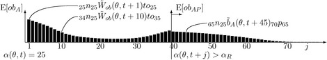
Figure 4 shows the different expected payment streams for the obligations arising before and after pension. The structure of the payment stream before pension has an distinctive shape. The peak at the beginning is explained by the high exit probabilities in the young years between 25 and 35 as described in Section 3.3. The valley at ages 40 to 55 (![]() ) is due to low exiting probability in combination with small invalidity probabilities. In the years just before pension, the effects of higher probability of falling invalid (Section 3.2) in combination with the very long compounding time (35 to 40 years) causes the expected obligations to rise again (Eq. (12)). The wealth which remains for pension (in the case of the member who stays in the pension fund until retirement) is taken for the calculation of the pension and is finally distributed over the expected lifetime as pensioner, as described by Eq. (14).
) is due to low exiting probability in combination with small invalidity probabilities. In the years just before pension, the effects of higher probability of falling invalid (Section 3.2) in combination with the very long compounding time (35 to 40 years) causes the expected obligations to rise again (Eq. (12)). The wealth which remains for pension (in the case of the member who stays in the pension fund until retirement) is taken for the calculation of the pension and is finally distributed over the expected lifetime as pensioner, as described by Eq. (14).
5 The pension funds’ projected liabilities
Pensioners’ liabilities consist of the payments of the remaining pensions. For active members, we distinguish between wealth ![]() at time t that the pension fund has accumulated for member θ which might be further accumulated until retirement and what might be paid out before that date. Here, we also include future projected contributions into the pension fund and the interest earned on the contributions for every year.
at time t that the pension fund has accumulated for member θ which might be further accumulated until retirement and what might be paid out before that date. Here, we also include future projected contributions into the pension fund and the interest earned on the contributions for every year.
5.1 Projected liabilities to pensioners
The annual benefit payment to pensioner θ is ![]() . The liability arising from this year’s pension payment to pensioner θ is
. The liability arising from this year’s pension payment to pensioner θ is ![]() . Annual payments are paid until the pensioner dies. They may be increased to account for rises in the cost of living after retirement. Mortality is the only uncertainty for pensioners.
. Annual payments are paid until the pensioner dies. They may be increased to account for rises in the cost of living after retirement. Mortality is the only uncertainty for pensioners.
Taking into account mortality, the expected liability arising from the payment of θ’s pension for next year is ![]() . The expected liabilities to θ in j years are
. The expected liabilities to θ in j years are
This is the survival probability for a year in j years ![]() , multiplied with the pension benefit
, multiplied with the pension benefit ![]() .
.
5.1.1 Projected future liabilities to active members before retirement
As seen in the case of obligations, the pension fund must take into account two possible types of future cash outflows for liabilities for its active members. Members either stay with the pension fund until retirement or will leave before that date. In retirement, they will receive a regular pension depending on their pension scheme. In case of a member leaving before retirement, the pension fund must transfer the full amount of accumulated wealth to the member’s new retirement plan. A considerable amount of funding is transferred in that manner and it cannot be disregarded since it is of importance with regard to short term liquidity planning. The liability arising for active member θ which is due to labour mobility is ![]() .
.
For member θ, with current accumulated wealth ![]() and the probability of leaving the pension fund
and the probability of leaving the pension fund ![]() , next year’s expected payment (due to labour mobility) is
, next year’s expected payment (due to labour mobility) is
In j years’ time, we expect the total payment of
where ![]() is the probability of the member to still be an active member in
is the probability of the member to still be an active member in ![]() years. Further,
years. Further, ![]() is the expected accumulated wealth of member θ at time
is the expected accumulated wealth of member θ at time ![]() according to Eq. (7) and
according to Eq. (7) and ![]() is the exit probability, given the age of member θ in year
is the exit probability, given the age of member θ in year ![]() .
.
5.2 Projected liabilities to active members after retirement
The liabilities arising after retirement to member θ who is active at time t but retired in year ![]() are
are ![]() . The expected liabilities in j years arising from the pension benefits are
. The expected liabilities in j years arising from the pension benefits are
This is the probability for reaching retirement age as a member of the pension fund given today’s age, ![]() , multiplied with the projected benefit payment for the active member
, multiplied with the projected benefit payment for the active member ![]() , and multiplied with the probability of surviving j years after retirement
, and multiplied with the probability of surviving j years after retirement ![]() . The projected pension benefit for the DC plan is given as
. The projected pension benefit for the DC plan is given as ![]() and for the DB plan with final projected wages
and for the DB plan with final projected wages ![]() .
.
6 Construction of the bucket structure
6.1 Bucket structure of expected undiscounted liabilities
The pension and labour mobility liability structure shows the pension fund liabilities, taking into account when the payment is due. Next year’s payments are calculated as the sum of all payments to current pensioners, plus the payments to the members that reach retirement age next year, plus all payments to active members leaving the pension fund next year due to labour mobility. This results in
 (19)
(19)with
where ![]() is the set of pension fund members in year t, and the indicator function
is the set of pension fund members in year t, and the indicator function ![]() if member θ is a pensioner in year t, and 0 otherwise. Furthermore the indicator function
if member θ is a pensioner in year t, and 0 otherwise. Furthermore the indicator function ![]() for member θ who is an active member in year t and retires in year
for member θ who is an active member in year t and retires in year ![]() ; zero otherwise, and
; zero otherwise, and ![]() for member θ who is an active member in year
for member θ who is an active member in year ![]() , zero otherwise. The factors
, zero otherwise. The factors ![]() ,
, ![]() and
and ![]() are the contributions of the members towards the buckets. The factor
are the contributions of the members towards the buckets. The factor ![]() is the projected pension for the active members at the time they retire. For a DC fund, it is given as
is the projected pension for the active members at the time they retire. For a DC fund, it is given as ![]() , and for a DB fund
, and for a DB fund ![]() , as defined in Eqs. (8) and (9).
, as defined in Eqs. (8) and (9).
The expected non-discounted payments due in j years are
 (20)
(20)where
This liability bucket structure shows the distribution of future cash flows and indicates what the undiscounted actual values of payments will be in future years.
6.2 Bucket structure of non-discounted obligations
Summarising from Sections 4.2 and 4.3 we can define the obligations arising from current accumulated wealth
 (21)
(21)where
As in Section 6.1, the indicator functions ![]() ,
, ![]() , and
, and ![]() delimitate pensioners, active members, and active members who became pensioners, respectively.
delimitate pensioners, active members, and active members who became pensioners, respectively.
6.3 Example: Buckets for pension fund liabilities and obligations
We consider four male members of the pension fund, ![]() , and
, and ![]() , B, C or D. In Table 1, we find their ages
, B, C or D. In Table 1, we find their ages ![]() , momentary salaries
, momentary salaries ![]() , projected salary at retirement
, projected salary at retirement ![]() , their momentary accumulated wealth
, their momentary accumulated wealth ![]() , projected wealth at retirement
, projected wealth at retirement ![]() , the probability of staying with the pension fund until retirement
, the probability of staying with the pension fund until retirement ![]() , and the expected survival probability for the next year
, and the expected survival probability for the next year ![]() .
.
Table 1 Pension fund members with their pension fund related data as explained in the text (annual salaries and wealth in thousands of CHF)

Figure 5 shows the expected payment streams for every member θ as the bucket structure. For the total pension liabilities (left column), the pension fund sums up all of the payments for every year as shown in the bottom graph. The sum of all the obligations is shown in the right column.

6.4 Bucket structure uncertainties
In previous sections, we derived expected values for liabilities and obligations for pensioners and active members based on life tables and other probabilistic figures. We assumed that the members are independent and are not influenced by the other members, thereby, for instance, neglecting slight differences between life tables for widowers and widows and their married peers. In this section, we derive the bucket uncertainties described by the variances of the bucket values.
When we look j years ahead, we can observe two possible outcomes for pensioners. Either they will die before j years have passed, or they will still live. An active member who is still active in j years is either still in the pension fund or has left before. And finally, active members who are older than the retirement age in j years, they could have left the pension fund before retirement, or, if they stayed until pension, there are the possibilities of their still being alive or being dead by now. In all three cases, we can observe two possible outcomes, so we can use binomial trees to model the probabilities and the outcomes, which in our case define the payments due to the members. Such a binomial tree is shown for the general case in Figure 6 where the probability of moving on the “up” branch is p invoking a payment of ![]() . The probability of moving on the “down” branch is given by
. The probability of moving on the “down” branch is given by ![]() , which invokes a payment of
, which invokes a payment of ![]() .
.

In this general case, the expected value of the payment in year ![]() is
is
with variance
We can define the probabilities and the payments which occur. The different cases are shown in Table 2. We use general forms for wealth and benefits (![]() and
and ![]() ), which can be specified further for the different cases, such as DB and DC funds, and active and passive members. All we need to know are the probabilities and the payments arising for the different cases of pensioners and active members in order to calculate uncertainties for the buckets.
), which can be specified further for the different cases, such as DB and DC funds, and active and passive members. All we need to know are the probabilities and the payments arising for the different cases of pensioners and active members in order to calculate uncertainties for the buckets.
Table 2 General case applied to pension fund probabilities and payments. Wealth ![]() and benefits
and benefits ![]() must be adjusted to the specific case (BD or DC)
must be adjusted to the specific case (BD or DC)

is the pensioner who survives another year in j years with probability ![]() and therefore gets paid a pension worth
and therefore gets paid a pension worth ![]() . In the case of death, with probability
. In the case of death, with probability ![]() , a payment of
, a payment of ![]() is due.
is due.
is the active member who is older than the retirement age in j years. This member gets paid a pension worth ![]() depending on the pension scheme (DB or DC). Further payment depends on projected earnings and wealth at retirement age and the probability of actually staying with the pension fund until pension, and then surviving the j years up to the current year,
depending on the pension scheme (DB or DC). Further payment depends on projected earnings and wealth at retirement age and the probability of actually staying with the pension fund until pension, and then surviving the j years up to the current year, ![]() .
.
is the active member, still active in j years. This member gets a payment of ![]() , the accumulated wealth in j years under the probability of staying in the fund for the last
, the accumulated wealth in j years under the probability of staying in the fund for the last ![]() years (
years (![]() ) and then leaving the pension fund in the jth year (with probability
) and then leaving the pension fund in the jth year (with probability ![]() ).
).
6.4.1 Uncertainties of obligations and liabilities to pensioners
The general benefit payment ![]() shown in Table 2 is replaced by the payment for pensioners
shown in Table 2 is replaced by the payment for pensioners ![]() . The general form for the expected value in Eq. (22) yields the expected value for the obligations
. The general form for the expected value in Eq. (22) yields the expected value for the obligations
We then insert the values of Table 2 into the general variance equation (23) for the variance for the pensioners obligations
 (25)
(25)For pensioners the obligations and liabilities are equal. Therefore, we can replace the ![]() by
by ![]() for the variance of the liabilities as follows
for the variance of the liabilities as follows
6.4.2 Uncertainties on obligations and liabilities to active members
By plugging the values for the active members (Cases “A” and “AP”) of Table 2 into the general variance formula (23) and replacing the general ![]() with
with ![]() and
and ![]() with
with ![]() , yields the expected value for “A”
, yields the expected value for “A”
and for “AP”
The variances are then for “A”
 (29)
(29)and for “AP”
For the uncertainties on the liabilities we must note that the projected wealth ![]() and projected pensions
and projected pensions ![]() themselves are stochastic due to the model used in Section 3.5.1, where there is a stochastic factor for cost-of-living increases in salaries. The variance for the liabilities is
themselves are stochastic due to the model used in Section 3.5.1, where there is a stochastic factor for cost-of-living increases in salaries. The variance for the liabilities is
 (31)
(31)where we use the short notation for projected wealth ![]() meaning
meaning ![]() . Similarly, “AP”
. Similarly, “AP”
![]() which depends on the pension fund (DB or DC). The values for the expected pensions
which depends on the pension fund (DB or DC). The values for the expected pensions ![]() can be calculated according to Eqs. (9) and (8).
can be calculated according to Eqs. (9) and (8).
6.4.3 Uncertainties of obligations and liabilities buckets
For the uncertainty of the buckets we sum up all individual uncertainties since every member is assumed to be an individual and not influenced by the other members. For the obligations buckets ![]() this results in
this results in
 (33)
(33)We use the indicator functions ![]() ,
, ![]() and
and ![]() as before, where
as before, where ![]() indicates that θ is a pensioner at time t,
indicates that θ is a pensioner at time t, ![]() indicates that θ is an active member in t and still so in
indicates that θ is an active member in t and still so in ![]() , and
, and ![]() indicates that θ is an active member in t and has retired at
indicates that θ is an active member in t and has retired at ![]() . The variances of
. The variances of ![]() ,
, ![]() and
and ![]() are in Eqs. (25), (29), and (30).
are in Eqs. (25), (29), and (30).
For uncertainties of the liabilities buckets ![]() we have the similar equation with the same indicator functions
we have the similar equation with the same indicator functions
 (34)
(34)where the variances of ![]() ,
, ![]() and
and ![]() are in Eqs. (26), (31), and (32).
are in Eqs. (26), (31), and (32).
6.4.4 Scenario generation for obligation and liability buckets
The future payments of the pension fund are stochastic since the fund faces several uncertainties that arise from its liability structure. The uncertainties arise from the risks individual members face as well as from macroeconomic factors such as wage inflation. To realistically evaluate future payments to members, the pension fund should know likely scenarios as well as worst-case and best-case scenarios. In terms of the bucket structure, obligation scenarios are ![]() and the liability scenarios are
and the liability scenarios are ![]() . Based on the expectations and variances for each individual bucket, we are able to simulate different scenarios. Since the liabilities are the summation of the individual’s contribution to the aggregated risk, we use the normal distribution to generate the scenarios. Alternatively, we can simulate all the different binomial random variables and aggregate them into the buckets. When the pension fund is large enough that the central limit theorem applies, the simulation based on the normal distribution is sufficient to generate statistically significant scenarios.
. Based on the expectations and variances for each individual bucket, we are able to simulate different scenarios. Since the liabilities are the summation of the individual’s contribution to the aggregated risk, we use the normal distribution to generate the scenarios. Alternatively, we can simulate all the different binomial random variables and aggregate them into the buckets. When the pension fund is large enough that the central limit theorem applies, the simulation based on the normal distribution is sufficient to generate statistically significant scenarios.
6.5 Total and discounted liabilities and obligations and current coverage ratios
The bucket structure for obligations and liabilities represents the actual, non-discounted values of the benefits which are due at given times in the future. By summing up all the buckets, we can calculate the total expected liabilities and obligations. We can also use the bucket structure to calculate the present value of the liabilities and obligations by discounting the buckets with the appropriate discounting factor. The present value of the buckets can be used to specify the current coverage ratio by comparing the present value with the present value of the current wealth.
6.5.1 Total expected obligations and liabilities to pensioners
The total (non-discounted) expected remaining pension outflow to a pensioner ![]() is
is
 (35)
(35)This is the sum of every year’s payment considering mortality. Values for ![]() in life tables are usually set to zero for very high ages (above a given
in life tables are usually set to zero for very high ages (above a given ![]() ). Since obligations and liabilities for pensioners are equal, the expected remaining pension outflow for pensioners is also equal for obligations and liabilities arising from these payments.
). Since obligations and liabilities for pensioners are equal, the expected remaining pension outflow for pensioners is also equal for obligations and liabilities arising from these payments.
6.5.2 Total expected obligations and liabilities to active members
For active members the total expected pension benefit outflow ![]() is
is
 (36)
(36)Here we sum up the yearly benefit payments after retirement ![]() with the uncertainty of mortality after pension
with the uncertainty of mortality after pension ![]() , while taking into account the possibility that the active member will not reach retirement age as member of the pension fund (
, while taking into account the possibility that the active member will not reach retirement age as member of the pension fund (![]() ). We also add the expected payments before retirement due to labour mobility (i.e., the probability of being in the fund until the year before the jth year (
). We also add the expected payments before retirement due to labour mobility (i.e., the probability of being in the fund until the year before the jth year (![]() ) multiplied with the projected wealth for the jth year (
) multiplied with the projected wealth for the jth year (![]() ) multiplied with the probability of leaving during the jth year (
) multiplied with the probability of leaving during the jth year (![]() ). From Eq. (36) both values for obligations and liabilities can be derived by using the general forms for benefits
). From Eq. (36) both values for obligations and liabilities can be derived by using the general forms for benefits ![]() and
and ![]() for wealth, respectively. For benefit payments
for wealth, respectively. For benefit payments ![]() is
is ![]() for the DC pension plan and
for the DC pension plan and ![]() for the DB plan.
for the DB plan.
6.5.3 Discounted obligations and liabilities buckets
Since the obligations and liabilities buckets have a term structure they can be discounted with the appropriate discount-factor and added up, which leads to the present value of obligations or liabilities. For an obligations bucket ![]() the present value is
the present value is
where ![]() is the interest rate used for discounting over j years. The present value of a liabilities bucket
is the interest rate used for discounting over j years. The present value of a liabilities bucket ![]() is
is
The present value of the pension fund’s total obligations then is given by the sum over all discounted buckets
 (39)
(39)where the number of buckets over which we sum up is given by the maximum reachable age minus the age of the youngest member (here 25 years) and ![]() is the discounting factor for the bucket in j years. As an example,
is the discounting factor for the bucket in j years. As an example, ![]() could be given by the yield curve of government bond interest rates with various maturities. Similarly, for liabilities
could be given by the yield curve of government bond interest rates with various maturities. Similarly, for liabilities
 (40)
(40)where the only difference is that we sum up the discounted liability buckets instead of obligations buckets.
6.5.4 Current coverage ratio
An important measure for the pension funds financial health is the coverage ratio. It is the present value of assets divided by the present value of liabilities. The coverage ratio is also found in the literature by the name of funding ratio (i.e., Rudolf and Ziemba (2004)). When the coverage ratio falls below one, there is currently not enough wealth in the pension fund to pay for the future liabilities.
The coverage ratio for the obligations is ![]() . Since obligations consist only of the payments due, based on compounding current wealth, we can write for the coverage ratio
. Since obligations consist only of the payments due, based on compounding current wealth, we can write for the coverage ratio
which is the ratio of current wealth to the present value of obligations. For liabilities, we need to take into account the present value of all future contributions into the pension fund, such that the coverage ratio for liabilities ![]() becomes
becomes
where ![]() is the present value of all future expected contributions. The two coverage ratios must be equal.
is the present value of all future expected contributions. The two coverage ratios must be equal.
7 The information value of the bucket structure
7.1 Information value of the life-insurance model
Based on this “life-insurance” model of a pension fund, we are able to analyse the relevant questions about the liabilities. For each individual member, we know the probability of exit from the pension fund. This helps us to answer questions such as mean time of membership for any given age and sex. This knowledge is crucial for the management of a fund, since we want to match the duration of the assets and liabilities. Furthermore, this knowledge allows the pension fund to earmark the wealth of each individual. Given the wealth of individual members and their exit probabilities, the obligation buckets indicate when and how much cash-flow can be expected from the current wealth. The description of uncertainty, i.e., the variances of the buckets, allows us to model scenarios for the obligations. For instance, active members might live longer than expected, which increases our liabilities.
Moreover, the different scenarios for inflation and wage levels help the pension funds to assess future contributions and the resulting liabilities. This feature, combined with the probabilistic description of the time of membership and exit from the fund, allows the pension fund to compute the expected cash-flows due to obligations and liabilities. The cash-flow description includes all major uncertainties that an individual member faces and which trigger a cash-flow from the fund. By assuming that all active members will stay in the fund until they reach the pension age, major cash-flows due to labour mobility and invalidity are not projected and the expected time of membership is overestimated. This might lead to inadequate investment decisions, since we assume longer maturity and a smaller intermediate outflow of funds than necessary.
Since we know the probabilities of the exit times, we are able to earmark the wealth and the contributions to the liability buckets. In this way, the pension fund’s wealth can be exactly matched to its liabilities. This in turn allows the fund to be managed according to its expected maturity. Furthermore, a sensible liquidity planning is another result, since provisions are taken for cash-flows due to labour mobility and invalidity. The idea of earmarking is used in Sections 8.5 and 8.6 as a central aspect of the pension fund optimisation.
7.2 Transparency and health of the pension plan
The earmarking of the individual wealth and of future contributions allows us to compute the coverage ratio for each bucket. Instead of working with a lump-sum coverage ratio, we can compute a term structure (maturity structure) of coverage ratios. This allows us to judge much better the financial “health” of the pension fund and indicates possible (unwanted) subsidies from one group to another. A lump-sum coverage ratio slightly below 100%, e.g., 95%, shows an under-funding of current obligations. When the under-funding is mostly concentrated on bucket coverage ratios with a long maturity, in which a higher investment into risky assets is possible, while the coverage ratios of the short maturities are above 100%, the under-funding must not be critical. In this situation, an increase in contributions is probably unnecessary. However, coverage ratios under 100% for buckets with short maturities indicate a clear financial stress situation. The bucket coverage ratio improves the assessment of the financial situation and allows for measured responses in a shortfall situation. The earmarking of current wealth and contributions allows the pension fund to detect possible cross-subsidies, where one group of members’ contributions is used to finance the liabilities (obligations) for another group of pension members. The method helps detecting such situations and shows the extent of such subsidies. The pension fund may also analyse how to correct such situations and evaluate their cost.
7.3 Utilisation of the information
The precise modelling of expected payments helps the pension fund simulate future scenarios and analyse its current situation. We can compute the influence of different fund structures, such as the guaranteed interest rate or studying differences between a DB plan or a DC plan. The precise modelling also increases the transparency of the fund structure and the utilisation of current pension fund wealth and contributions. Moreover, different contribution schemes, which may depend, for example, on the coverage ratio or the current underlying economic situation, can be evaluated. Scenarios of future trajectories of assets and liabilities may serve as inputs to optimise the asset allocation. The bucket structure simulation together with a simulation of the asset allocation, supports the pension fund management in determining critical scenarios, such as high labour mobility while asset returns are falling. In this way, concentrations of hidden risks can be detected and addressed early. The term structure of obligations allows us to use classical asset liability techniques such as duration matching and immunisation.
7.4 Pooling of pension funds
Another important question this method helps to analyse is the pooling of different pension funds. When two or more pension funds want to pool their operations, we can judge the situation much better with the life-insurance modelling technique. We can assess the obligations and liability buckets which arise from the pooling and compare this to the individual pension fund’s situation. This helps to determine for which fund such pooling is beneficial and for which it is not. For example, a pension fund with low labour mobility combined with a fund with high labour mobility and a similar distribution of members ages, might result in a more manageable pension fund, since for one fund it reduces the duration of liabilities and for the other it increases it. Additionally, the cash-flows become smoother over time and less volatile for each given period.
7.5 Cost vs. benefits of the model
This modelling approach of pension fund obligations and liabilities is costly in the sense that considerable data is needed for the analysis. However, the insights gained by this type of model justifies the additional work needed. Especially in long-term optimisation and analysis, a precise description of the liabilities ensures applicable and robust decisions.
8 Asset–liability management optimisation
8.1 Introduction
The globalisation of financial markets and the introduction of various new and complex products, such as options or other structured products, have significantly increased the volatility and risk for participants in the markets. Moreover, advances in communication technology and computers have dramatically increased the reaction speed of financial markets to world events. This has occurred within Switzerland, the country in which the fund resides, as well as across markets internationally. The long-term nature of a pension fund amplifies the financial rewards for good decisions as well as the penalties for bad decisions. Furthermore, the dynamic and uncertain nature of both the asset and the liability trajectories greatly complicates the investment problem. Therefore, the need to integrate the liability and the asset management has dramatically increased.
In recent years, a growing number of applications of integrated risk management have emerged. Insurance companies and pension funds pioneered these applications, which include the Russell–Yasuda investment system (Cariño et al., 1994), the Towers Perrin System (Mulvey, 1995), and the Siemens Austria Pension Fund (Ziemba (2003) and Geyer et al. (2004)). In each of the applications, the investment decisions are linked with liability choices, and the system’s funds are maximised over time using multi-stage stochastic programming. The integrated risk management approach is therefore the best suited way of managing a pension fund. It includes the dynamics of the assets, the dynamics of the liabilities, the long-term nature of the pension fund, and the uncertainty faced by the fund.
Most financial planning systems today still rely on the classical mean-variance framework pioneered over 50 years ago. Despite its huge success, the single-period setting possesses some significant deficiencies. First, it is difficult to use in a long-term application where investors are able to rebalance their portfolio frequently. Second, for situations where investors face liabilities or goals at specific future dates, the investment decisions must be taken with regard to the dynamics and time structure involved. The multi-period approach may also provide superior performance over the single-period approach, see Dantzig and Infanger (1993). Third, the definition of risk, such as variance or semi-variance, does not transfer any information regarding the chances of matching the obligations or goals. Furthermore, variance or semi-variance are not coherent risk measures in the sense of Artzner et al. (1999). Fourth, the mean variance framework is extremely sensitive to the model inputs, i.e., mean values and covariances. Fifth, the mean variance framework cannot easily handle issues such as taxes and transaction costs.
Nevertheless, economic growth theory recommends that a multi-period investor should maximise the expected logarithmic wealth at each time period, as suggested by Luenberger (1998). However, it has been shown in Rudolf and Ziemba (2004) that a logarithmic utility may lead to a too high risk tolerance. In addition, the theory depends on various assumptions such as no transaction cost, i.i.d. asset returns, and neither liabilities nor in- or outflows to be time-dependent. When these assumptions are violated, as they are in the case of pension funds, a multi-period setting is the appropriate framework to handle such a problem.
For all these stated reasons, it is necessary to use a dynamic multi-period optimisation rather than the classical single-period framework.
8.2 Multi-period asset model
Many different formulations of multi-period investment problems can be found in the literature, see Ziemba and Mulvey (1998), Kall and Wallace (1994), Kusy and Ziemba (1986), or Louveaux and Birge (1997). We adopt the basic model formulation presented in Mulvey and Simsek (2002) and Mulvey and Shetty (2004), with various modifications. The asset and liability management horizon consists of τ time steps represented by ![]() , where t is the current time and
, where t is the current time and ![]() is the planning horizon. At every time step, the pension fund is able to make a decision regarding its investments and faces the inflow of funds due to contributions and outflows due to obligations.
is the planning horizon. At every time step, the pension fund is able to make a decision regarding its investments and faces the inflow of funds due to contributions and outflows due to obligations.
The investment classes are defined as the set ![]() . This set should reflect all important asset classes, such as stocks (large, small, international, emerging markets), bonds, cash, and real estate. The asset classes chosen for the optimisation should reflect important market segments and should be available as investable security, such as index funds or future contracts. Examples are the Swiss Performance Index, which tracks the largest 100 Swiss stocks or the S&P 500 in the US.
. This set should reflect all important asset classes, such as stocks (large, small, international, emerging markets), bonds, cash, and real estate. The asset classes chosen for the optimisation should reflect important market segments and should be available as investable security, such as index funds or future contracts. Examples are the Swiss Performance Index, which tracks the largest 100 Swiss stocks or the S&P 500 in the US.
The uncertainties faced by the pension fund, either from the investments or from the liabilities, are modelled by the so-called scenario approach. By utilising a sufficiently large number of scenarios, we are able to represent all of the random effects the pension fund faces. The scenarios are defined as the set S that represents a reasonable description of the future uncertainties. A scenario ![]() describes a unique path through consecutive nodes of the scenario tree as depicted in Figure 7. Many mathematical techniques exist to generate scenarios. Most authors use various econometric methods to describe future asset returns. Examples in the case of asset liability management applications include Dert (1998), Boender (1997), Boender, van der Aalst and Heemskerk (1998), Koivu, Pennanen and Ranne (2005), and Wilkie (1995). An important aspect of the scenario modelling is its forward-looking and dynamic character. Instead of analysing historical returns, such as mean and covariances, we can build forward-looking models which evaluate the pension fund’s situation. The idea is to construct sets of scenarios that represent the pension fund’s unique situations, such as possible assets, cost, liabilities, and legal requirements.
describes a unique path through consecutive nodes of the scenario tree as depicted in Figure 7. Many mathematical techniques exist to generate scenarios. Most authors use various econometric methods to describe future asset returns. Examples in the case of asset liability management applications include Dert (1998), Boender (1997), Boender, van der Aalst and Heemskerk (1998), Koivu, Pennanen and Ranne (2005), and Wilkie (1995). An important aspect of the scenario modelling is its forward-looking and dynamic character. Instead of analysing historical returns, such as mean and covariances, we can build forward-looking models which evaluate the pension fund’s situation. The idea is to construct sets of scenarios that represent the pension fund’s unique situations, such as possible assets, cost, liabilities, and legal requirements.

Let ![]() be the amount of wealth invested in instrument i at the beginning of the time step
be the amount of wealth invested in instrument i at the beginning of the time step ![]() under scenario s. The units used are the pension fund’s home currency (Swiss Francs). Foreign assets, either hedged or unhedged, are also denoted in the fund’s home currency. At time
under scenario s. The units used are the pension fund’s home currency (Swiss Francs). Foreign assets, either hedged or unhedged, are also denoted in the fund’s home currency. At time ![]() the total wealth of the fund is
the total wealth of the fund is
where ![]() denotes the total wealth under scenario s. Given the returns of each investment class, the asset values at the end of the time period are
denotes the total wealth under scenario s. Given the returns of each investment class, the asset values at the end of the time period are
where ![]() is the return of investment class i at time
is the return of investment class i at time ![]() under scenario s. The returns are obtained from the scenario generation system. Therefore,
under scenario s. The returns are obtained from the scenario generation system. Therefore, ![]() is the ith asset value at the end of the time period
is the ith asset value at the end of the time period ![]() under scenario s. For stocks, assume that dividends are part of the return and that they are automatically reinvested. The sales or purchases of assets occur at the beginning of the time period, where
under scenario s. For stocks, assume that dividends are part of the return and that they are automatically reinvested. The sales or purchases of assets occur at the beginning of the time period, where ![]() denotes amount of asset i sold at time
denotes amount of asset i sold at time ![]() under scenario s, and
under scenario s, and ![]() denotes the purchase of asset i at time
denotes the purchase of asset i at time ![]() under scenario s. The asset balance equation for each asset is
under scenario s. The asset balance equation for each asset is
where ![]() is the proportional transaction cost of asset i. We make the assumption that the transaction costs are not a function of time, but depend only on the investment class involved. This assumption can be easily relaxed to include a time dependency. We treat the cash component of our investments as a special asset. The balance equation for cash is
is the proportional transaction cost of asset i. We make the assumption that the transaction costs are not a function of time, but depend only on the investment class involved. This assumption can be easily relaxed to include a time dependency. We treat the cash component of our investments as a special asset. The balance equation for cash is
 (46)
(46)where ![]() is the cash account at time
is the cash account at time ![]() under scenario s,
under scenario s, ![]() and
and ![]() are the contributions received by the fund and the outflows due to payments by the fund at time
are the contributions received by the fund and the outflows due to payments by the fund at time ![]() under scenario s, respectively. The cash account equals the interest rate earned from the cash account’s value of the last period, plus all money earned from sales of assets, minus all money used for the purchase of assets, plus the contributions minus the payments due to obligations of the fund. Furthermore, we restrict all assets, including the cash account, to be non-negative, i.e.,
under scenario s, respectively. The cash account equals the interest rate earned from the cash account’s value of the last period, plus all money earned from sales of assets, minus all money used for the purchase of assets, plus the contributions minus the payments due to obligations of the fund. Furthermore, we restrict all assets, including the cash account, to be non-negative, i.e., ![]() . This means that we do not allow for any borrowing. This restriction may be dropped in other situations.
. This means that we do not allow for any borrowing. This restriction may be dropped in other situations.
All variables in Eqs. (43)-(46) are dependent on the actual scenario s. These equations could be decomposed into subproblems for each scenario where we anticipate which scenario will evolve. To model reality, we must, however, impose non-anticipativity constraints. All scenarios which inherit the same past up to a certain time period must evoke the same decisions in that time period, otherwise the non-anticipativity requirement would be violated. So, ![]() when s and
when s and ![]() have same past until time
have same past until time ![]() .
.
Another way of imposing the non-anticipativity requirement is to use control policies which do not depend on the future path of the assets and liabilities. Such a policy is the fixed-mix strategy, where we require that a fixed proportion of the wealth is invested in a certain asset (Ziemba (2003)). Alternatively, we could also allow that the mix is time-varying, but still independent of the scenarios. This results in a dynamic-mix (or time-varying mix) strategy. The fixed-mix strategy has a thorough theoretical underpinning in the case where the asset returns show no inter-temporal dependency. This is a well-known result from continuous-time finance and stochastic control theory as derived by Merton (1969, 1973). When asset returns exhibit inter-temporal dependencies, which is the case when asset returns are described by factor models, the constant-mix is not the optimal asset allocation strategy. For this case, Campbell, Rodriguez and Viceira (2004), and Herzog et al. (2004) show, by employing optimal stochastic control theory, that a dynamic-mix is the optimal asset allocation strategy. The fraction of wealth at time ![]() invested in the ith asset is
invested in the ith asset is
For the fixed-mix strategy, ![]() , since it does not depend on time. The mix strategies reduce the number of decision variables to a large extent, but they introduce nonlinearity into the problem. To analyse Eq. (47), we use Eqs. (43)-(46) and obtain
, since it does not depend on time. The mix strategies reduce the number of decision variables to a large extent, but they introduce nonlinearity into the problem. To analyse Eq. (47), we use Eqs. (43)-(46) and obtain
 (48)
(48)The asset sales and purchases under each scenario and at any time can be computed in this manner. The wealth at time ![]() before rebalancing minus the net transaction costs is divided among the N assets according to the mix rule
before rebalancing minus the net transaction costs is divided among the N assets according to the mix rule ![]() . The various nonlinearities in Eq. (48) are visible such as the term
. The various nonlinearities in Eq. (48) are visible such as the term ![]() .
.
When we neglect transaction costs and use the mix rules, the evolution of the wealth can be computed from
 (49)
(49)The system’s N balance equations and constraints are reduced to a one-dimensional equation and we do not need to compute the sales and purchases for each scenario and time in order to know the evolution of the fund’s wealth.
8.3 Optimisation objectives for the pension fund asset–liability management
We outline the general objectives of the fund and how they can be translated into objective functions and constraints. Since we deal with decisions under uncertainty, the definition of risk for the pension fund is crucial for the appropriate asset liability management optimisation. From the regulatory point of view in Switzerland, the health of a pension fund is judged by the criteria known as (current) coverage ratio. The interest rate for discounting the liabilities set by the regulators is called technical interest rate. The coverage ratio is required to be above 100% and various measures have to be taken in case it falls below 100%. These measures range from changes in the investment strategy to increases in contributions from both employer and employees up to in the worst case, the termination of the fund.
Many coherent risk measures have been found, such as maximum loss or conditional Value-at-Risk (CVaR). The risk measure used for asset liability management applications, however, must be tailored to the specific situation and the specific objectives of the fund. Standard coherent risk measures, such as CVaR, can be used in ALM situations, when applied to the fund’s net wealth, e.g., the sum of the assets minus all the remaining liabilities (obligations). CVaR penalises linearly all events which are below the VaR limit for a given confidence level. The inherent VaR limit is a result of the CVaR optimisation, see Rockafellar and Uryasev (2000) and Rockafellar and Uryasev (2002). The VaR limit therefore depends on the confidence level chosen and the shape of the distribution. The VaR limit (quantile) may be a negative number, i.e., a negative net wealth result. In the situation of a pension fund, we do not only want to penalise scenarios that are smaller than a given quantile, but all scenarios where the net wealth is non-positive. The most important objective of the pension fund is to meet its obligations and achieve a positive net wealth. For these reasons, we define risk as a penalty function for the net wealth. The net wealth can be either measured in absolute terms, e.g., Swiss Francs, or in relative terms, i.e., as a percentage of the obligations. Second, we want to penalise small “non-achievement” of obligations differently from large “non-achievement”. Therefore, the penalty function should have an increasing slope with increasing “non-achievement”. Third, the penalty function should be a convex function. The risk of the pension plan is measured as one-sided downside risk based on non-achievement of the obligations.
The expectation is a convexity preserving operation. The penalty function is not a coherent risk measure. However, the conditional expectation of the non-positive net wealth is coherent and coincides with the penalty function where only one slope with an incline of one is used. The reason why the general penalty function is not coherent is that it is not a monetary measure of potential losses, but rather a non-monetary (artificial) number of non-achievement. The advantage of the penalty function approach is that large losses are more heavily penalised than smaller losses. For optimisation purposes, we can use the penalty function for the terminal net wealth of the fund or compute the penalty function for each future time. A practical method is to define a non-negative weighted sum of the penalty functions for all time. In this way we control the risk of non-achievement in a multi-period setting.
The second objective of the fund is to achieve a surplus from the funds under management. For this reason, we want to maximise the expected net wealth. We either formulate this goal as a terminal date objective, or again, as a weighted sum over all time periods.
8.4 Optimisation approaches for multi-period ALM models
For the mathematical model of asset and liability dynamics described in Section 8.2, many different optimisation methods exist. Here, we will briefly describe two different approaches, namely the stochastic programming approach and the dynamic stochastic control approach. Other possible optimisation techniques, such as dynamic programming, are not discussed here. For our pension fund application we briefly describe a system which sets up an account for each liability which is funded, in order to cover the associated obligation. Each account is individually managed and funded.
8.4.1 Stochastic programming approach
The stochastic programming approach finds the optimal sales variables ![]() and the optimal purchase variables
and the optimal purchase variables ![]() given the current time and scenario including the non-anticipativity constraints. By inspecting Eqs. (43)-(46), we see that these equations are linear. Furthermore, when we use a linear objective function, then the optimisation problem becomes a large-scale linear programming (LP) problem. The objective function is
given the current time and scenario including the non-anticipativity constraints. By inspecting Eqs. (43)-(46), we see that these equations are linear. Furthermore, when we use a linear objective function, then the optimisation problem becomes a large-scale linear programming (LP) problem. The objective function is
where the ![]() represents all remaining obligations at the end of the planning horizon under scenario s,
represents all remaining obligations at the end of the planning horizon under scenario s, ![]() denotes the piecewise linear penalty function, and
denotes the piecewise linear penalty function, and ![]() denotes the probability of scenario s. Alternatively, we can formulate the objective function based on the liability buckets. The penalty function is also applied to net wealth, i.e.,
denotes the probability of scenario s. Alternatively, we can formulate the objective function based on the liability buckets. The penalty function is also applied to net wealth, i.e., ![]() . The objective (50) is a piecewise linear function of the decision variables. Many specialised algorithms exist to solve this special form LP, such as the L-shaped algorithm, see van Slyke and Wets (1969), Kall and Wallace (1994), Birge et al. (1994), and Birge and Holmes (1992). Other approaches, known not to work satisfyingly, are known as the progressive hedging algorithm, see Rockafellar and Wets (1991), Berger, Mulvey and Ruszczynski (1994), and Barro and Canestrelli (2005).
. The objective (50) is a piecewise linear function of the decision variables. Many specialised algorithms exist to solve this special form LP, such as the L-shaped algorithm, see van Slyke and Wets (1969), Kall and Wallace (1994), Birge et al. (1994), and Birge and Holmes (1992). Other approaches, known not to work satisfyingly, are known as the progressive hedging algorithm, see Rockafellar and Wets (1991), Berger, Mulvey and Ruszczynski (1994), and Barro and Canestrelli (2005).
The advantage of the stochastic programming approach over the dynamic stochastic control approach is that the decisions are computed similarly to a feedback control system. Given the new realisations, i.e., when we know the current state of our system, we have a prescribed rule of actions that helps us to achieve the objectives. The decision rule observes the actual path our system has taken in the past and uses the conditional information of the current state for the future uncertainty. Furthermore, under different scenarios, the fraction of wealth invested in the different asset classes differs, which sets this apart from the fixed-mix approach.
The main disadvantage is that for systems with many future time periods, the number of scenarios ![]() , where
, where ![]() is the number of branches at each time step j, increase exponentially. Furthermore, developing a representative tree of scenarios is a challenging research field. There are several objectives to meet when building a stochastic scenario tree. The scenarios must be based on sound and realistic economic principles. Basic observations from econometrics should be included, such as volatility clustering in equity markets or mean reversion of interest rates. Projections of future scenarios should be investigated with regard to how well they fit past observations. The main feature of scenario generation is to reflect a universe of possible outcomes. This must include likely scenarios, as well as best and worst case scenarios.
is the number of branches at each time step j, increase exponentially. Furthermore, developing a representative tree of scenarios is a challenging research field. There are several objectives to meet when building a stochastic scenario tree. The scenarios must be based on sound and realistic economic principles. Basic observations from econometrics should be included, such as volatility clustering in equity markets or mean reversion of interest rates. Projections of future scenarios should be investigated with regard to how well they fit past observations. The main feature of scenario generation is to reflect a universe of possible outcomes. This must include likely scenarios, as well as best and worst case scenarios.
8.4.2 Dynamic stochastic control approach
The dynamic control approach works by using control policies that are independent of the current and future scenarios. The basic decision variables are fixed-mix or dynamic-mix variables. The main advantage of the stochastic control policies is that they reduce the size of the problem drastically and that they are well understood by investment professionals. Furthermore, theoretical results from continuous-time finance support this approach, see Merton (1992). By allowing dynamic-mix strategies, i.e., the mix is not constant throughout the planning horizon, we can also introduce feedback into the system. This feedback depends on the time dependencies of the asset returns.
The main disadvantage of the stochastic control strategies is that they introduce nonlinearities into the optimisation problem regardless of the functional form of the objective function. Very often we are also faced with the situation of a non-convex nonlinear optimisation, which requires specialised global solution algorithms, see Maranas et al. (1997) and Konno and Wijayanayake (2002), or other global optimisation techniques, such as genetic algorithms.
8.4.3 Application to the problem of a pension fund
The pension fund investment problem is marked by its long-term nature and its term structure of payments due to pensions and other obligations. In Section 8.3 we briefly outlined the fund’s ALM objectives.
To match all the goals for each obligation bucket (or liability bucket), a corresponding account is set up. The account consists of several assets which are to provide the funds needed to pay the obligation of that bucket. The accounts have different terminal dates depending on maturity of the associated bucket. Due to the actuarial treatment of the various risks, we know the distribution of possible exit times of members and, therefore, are able to earmark the contributions to the different liability buckets.
Furthermore, each individual account has its own investment policy which depends not only on the risk-aversion but also on the investment time horizon. Using stochastic control theory, Brennan, Schwartz and Lagnado (1997) and Campbell and Viceira (2002) have shown that the investment policy depends both on risk aversion and time horizon. For each account, a part of the current wealth is earmarked. The decision variables are therefore, the earmarking of funds for the accounts and the investment policy of the accounts. To optimise the entire fund and not only each individual account, the objective function is the superposition of surplus wealth of all of the accounts and the superposition of penalty functions of all of the accounts. By using the accounts, we can translate the preferences of the individual pension fund members into the goals and objectives of the pension fund. The life-style hypothesis, see Cairns, Blake and Dowd (2003), is thus realised across the pension fund. Moreover, in this way we can control the coverage ratio for each individual bucket. The coverage ratio for the entire fund is not as meaningful as the bucket coverage ratio together with the bucket term structure.
Alternatively, we could set up an asset liability management optimisation for the entire wealth of the fund. From the liability model and the bucket structure, we have a stochastic model for the time structure of contributions and payments due to liabilities. The optimisation then determines an investment policy for the entire fund. The fund’s objective in terms of risk and surplus can similarly be incorporated. However, using the accounts and buckets better matches the individuals’ preferences with the overall management of the pension fund. Furthermore, the earmarking of funds is an important decision variable which determines the health of the fund, i.e., coverage ratios for buckets provide much clearer information on possible shortfalls and on the time horizon in which they might occur than the lump-sum coverage ratio.
In Section 8.5, we propose an optimisation for the asset obligation management which does not take transaction cost into account and uses relative measures for the surplus and the risk involved. This solution focuses on the management of current funds (wealth) and the obligations that arises therefrom. Since we do not consider any future contributions, the pension fund’s wealth must be invested to match the obligations. In Section 8.6, we work with absolute measures and include transaction costs. We also include future contributions and therefore match the current funds and contributions with the resulting liabilities. Both optimisations use the idea of buckets, accounts, and earmarking. The optimisation approach is the dynamic stochastic control approach.
8.5 Optimisation of asset obligation management with earmarking and investment policy without transaction costs
We describe an optimisation for the pension fund’s asset obligation management based on the projected obligations and current wealth of the pension fund. For each obligation bucket, we set up an account to manage the funds earmarked for the specific obligation. We assume that transaction costs and market impact can be neglected.
8.5.1 Projected account value
From the life insurance model of the pension fund the future guaranteed payments for each obligation bucket are known. To meet these obligations, the pension fund assigns funds from its current wealth and determines an investment policy. All accounts are denoted by the set J. For each bucket we allocate a part of the current wealth using
where ![]() is the current wealth,
is the current wealth, ![]() is the wealth allocated to cover the obligations in the jth bucket, and
is the wealth allocated to cover the obligations in the jth bucket, and ![]() is a fraction of the current wealth. The following constraints apply
is a fraction of the current wealth. The following constraints apply
 (52)
(52)For ![]() we take the jth bucket out of consideration since there are no liabilities to be covered for this bucket. The fraction of wealth assigned to the jth bucket should be invested so that the guaranteed future obligations are matched or even exceeded. The projected account value assigned to jth bucket is
we take the jth bucket out of consideration since there are no liabilities to be covered for this bucket. The fraction of wealth assigned to the jth bucket should be invested so that the guaranteed future obligations are matched or even exceeded. The projected account value assigned to jth bucket is
where ![]() is the account for the jth bucket and
is the account for the jth bucket and ![]() is the number of rebalancing periods until the account matures at time
is the number of rebalancing periods until the account matures at time ![]() . The returns of the individual assets at time
. The returns of the individual assets at time ![]() under scenario s are
under scenario s are ![]() . Assume that there exists a finite number of scenarios
. Assume that there exists a finite number of scenarios ![]() . Then
. Then ![]() is the fraction of bucket wealth invested into the lth asset. Assume that the investments into the N assets are rebalanced at every rebalancing period. To write (53) more concisely, we stack all returns plus one in the vector
is the fraction of bucket wealth invested into the lth asset. Assume that the investments into the N assets are rebalanced at every rebalancing period. To write (53) more concisely, we stack all returns plus one in the vector ![]() and write
and write ![]() . Eq. (53) becomes
. Eq. (53) becomes
We assume that no transaction cost or taxes apply, which is of course an approximation of reality. However, there are investable securities with minimal brokerage fees, such as futures on indices. Furthermore, we tacitly assume that our trading impact is small enough that we do not influence the asset prices.
The logarithm of both sides of (54) yields
 (55)
(55)where ![]() is the logarithm of
is the logarithm of ![]() . The decision variables for the jth account are current investment policy
. The decision variables for the jth account are current investment policy ![]() and the earmarking of funds
and the earmarking of funds ![]() .
.
Theorem 1 The logarithmic value of the jth account ![]() is concave with respect to the decision variables
is concave with respect to the decision variables ![]() and
and ![]() .
.
Proof By straight forward calculation verify that the Hessian of Eq. (55) is negative semi-definite.
8.5.2 Optimisation problem
The aim of the fund is to meet its obligations with high certainty while attempting to generate a surplus. Therefore, we define risk as the possibility that the account value does not cover the obligations. The coverage ratio at the time of the maturity of the bucket is
where ![]() denotes the future obligations in bucket j under scenario s and
denotes the future obligations in bucket j under scenario s and ![]() is the coverage ratio at maturity. Taking the logarithm of (56) yields
is the coverage ratio at maturity. Taking the logarithm of (56) yields
The log-coverage ratio is larger than zero if the account’s fund is larger than the earmarked obligations and smaller than zero if the fund’s wealth does not cover the obligations. If the account value does not cover the obligations, the log-coverage ratio is a negative number.
The number is similar to a total percentage number of either over- or underachievement minus 100%, e.g., a coverage ratio of 120% results in a log-coverage ratio number of 18.23%. The log-coverage-ratio actually slightly underestimates coverage ratios above 100% and overestimates coverage ratios below 100%, e.g., a coverage ratio of 80% results in a log-coverage-ratio number of ![]() . In this manner, the measure errs on the conservative side, since it underestimates surpluses and overestimates shortfalls. When we divide the log-coverage number by the investment periods of this account, we obtain a compounded return number.
. In this manner, the measure errs on the conservative side, since it underestimates surpluses and overestimates shortfalls. When we divide the log-coverage number by the investment periods of this account, we obtain a compounded return number.
We define the aggregated weighted shortfall under scenario s as the non-negative summation of all individual weighted negative log-coverage ratios for each bucket, or mathematically as
 (58)
(58)Here ![]() is a weighting factor for each bucket. The risk of the pension plan is measured as a one-sided downside risk based on non-achievement of the obligations. As penalty function we choose piecewise linear function
is a weighting factor for each bucket. The risk of the pension plan is measured as a one-sided downside risk based on non-achievement of the obligations. As penalty function we choose piecewise linear function
 (59)
(59)Here ![]() and
and ![]() are slopes of the penalty function and
are slopes of the penalty function and ![]() is the point where the penalty increases more steeply, as discussed in Section 8.3. In this way, we do not penalise the achievement or over-achievement of the obligation, but penalise the shortfall. The shortfall is divided into two sections, one for slightly missing the obligations and one for larger deviations from the obligations.
is the point where the penalty increases more steeply, as discussed in Section 8.3. In this way, we do not penalise the achievement or over-achievement of the obligation, but penalise the shortfall. The shortfall is divided into two sections, one for slightly missing the obligations and one for larger deviations from the obligations.
The surplus of the pension fund is computed with the help of the aggregated weighted surplus
 (60)
(60)where ![]() is a weighting factor of the surplus of each bucket. The weighting factors are also necessary to interpret the result since the surpluses arise from buckets with very different time periods. The objective function is the expected penalty minus the weighted expected surplus, given by
is a weighting factor of the surplus of each bucket. The weighting factors are also necessary to interpret the result since the surpluses arise from buckets with very different time periods. The objective function is the expected penalty minus the weighted expected surplus, given by
where ![]() is the weighting factor for the aggregated surplus and
is the weighting factor for the aggregated surplus and ![]() denotes the probability for each scenario. The optimisation problem is to choose the investment policy for each bucket (
denotes the probability for each scenario. The optimisation problem is to choose the investment policy for each bucket (![]() ) and the fraction of pension fund wealth earmarked for the jth bucket (
) and the fraction of pension fund wealth earmarked for the jth bucket (![]() ), while minimising the objective function. This also allows us to control the coverage ratio for each bucket. Furthermore, we impose linear (or convex) constraints on the decision variables. For example, we do not allow short-selling or leverage for the investment policy for each bucket. The earmarking of funds for the different buckets must stay within a given range in order to keep the current coverage ratio within predetermined levels. Furthermore, we need to observe institutional, legal, and regulatory constraints. For instance, in Switzerland a pension fund is prohibited from investing more than 30% of its funds in the Swiss stock market.
), while minimising the objective function. This also allows us to control the coverage ratio for each bucket. Furthermore, we impose linear (or convex) constraints on the decision variables. For example, we do not allow short-selling or leverage for the investment policy for each bucket. The earmarking of funds for the different buckets must stay within a given range in order to keep the current coverage ratio within predetermined levels. Furthermore, we need to observe institutional, legal, and regulatory constraints. For instance, in Switzerland a pension fund is prohibited from investing more than 30% of its funds in the Swiss stock market.
The optimisation problem to determine the investment policy and the funding of each bucket is

Here ![]() denotes the set of all linear or convex constraints for the investment policy and
denotes the set of all linear or convex constraints for the investment policy and ![]() the set of all linear or convex constraints for the earmarking of funds.
the set of all linear or convex constraints for the earmarking of funds.
Theorem 2 The optimisation problem given in (62) is a convex optimisation problem with respect to the decision variables ![]() and
and ![]() .
.
Proof In Theorem 1 we have shown that ![]() is a concave function with respect to the decision variables. Furthermore, the aggregated weighted shortfall (58) is convex with respect to the decision variables since
is a concave function with respect to the decision variables. Furthermore, the aggregated weighted shortfall (58) is convex with respect to the decision variables since ![]() is convex and the nonnegative weighting preserve convexity, see Boyd and Vandenberghe (2004, 3.2.1). The penalty function (59) is piecewise linear which again preserves the convexity. The expectation operation over all scenarios also preserves the convexity. The expected penalty part of the objective function is thus convex. The aggregated weighted surplus (60) is a concave function with respect to the decision variables, but the multiplication with −γ (
is convex and the nonnegative weighting preserve convexity, see Boyd and Vandenberghe (2004, 3.2.1). The penalty function (59) is piecewise linear which again preserves the convexity. The expectation operation over all scenarios also preserves the convexity. The expected penalty part of the objective function is thus convex. The aggregated weighted surplus (60) is a concave function with respect to the decision variables, but the multiplication with −γ (![]() ) changes this part to a convex function. The expectation operation preserves the convexity of the negative weighted surplus. Furthermore, we assume that
) changes this part to a convex function. The expectation operation preserves the convexity of the negative weighted surplus. Furthermore, we assume that ![]() and
and ![]() are both sets that describe linear or convex inequalities and equalities.
are both sets that describe linear or convex inequalities and equalities.
The optimisation problem is convex and can be thus solved by a suitable convex programming software package. The main advantage is that we arrive at a unique solution and do not need specialised algorithms to search for the global solution. The problem can be solved with many decision variables, which allows the pension funds to set up a suitable number of accounts and include a wide array of investment vehicles.
8.5.3 Control algorithm
The asset obligation optimisation prescribes an investment rule for each bucket. However, each year the pension fund pays out the obligation of the first year bucket and collects all contributions. The bucket structure is calculated anew and the buckets for the new obligations are established. Because of the contributions, the exit and entry of members, and the effect of the guaranteed interest rate, the obligations look different from the last year’s obligations, even when we take into account that the second-year obligation is now the new first-year obligation and so on.
For this reason, we have to calculate the optimisation problem (62) again. This recalculation introduces feedback into the problem, since we base our solution on the latest states of our assets and obligations. Moreover, when the rebalancing frequency is higher than the recalculation frequency of the obligations, we also solve the problem for the intermediate time periods. We then base the new optimisation also on the latest investment results and therefore, the pension fund is managed with a feedback control approach. The approach is shown in Figure 8. In control engineering this approach is known as either model predictive control, or receding horizon control, or sometimes as open-loop feedback control. This approach has thorough theoretical underpinnings, see Garcia, Prett and Morari (1989) and Bemporad et al. (2002) for deterministic applications. References to the model predictive control approach in stochastic optimisation problems in the area of finance include Herzog, Dondi and Geering (2004), Herzog, Geering and Schumann (2004), and Meindl and Primbs (2004), and, in other areas, e.g., Kouvaritakis, Cannon and Tsachouridis (2004).

By solving the problem for each time step again, we solve the feedback problem for the given state and time. The model predictive control approach always solves the optimisation problem conditional on the latest measured information. The optimisation problem corresponds to an open-loop control solution. Furthermore, at each resolving of the optimisation problem, we may also recalculate the asset return model. We can refit the asset return model to the data set that includes the new information. In this manner, we adapt our economic models to the new situation. Similarly we can also include new observations from our liability models, even though demographic statistics tend to change rather slowly. This enables us to build a truly adaptive control algorithm for the pension fund optimisation.
8.6 Asset–liability management optimisation with earmarking and investment policy and transaction costs
We describe a pension fund asset liability optimisation based on the projected liabilities and projected contributions. As described in Section 8.5, for each liability bucket we set up an account to manage the funds earmarked for the specific liability. Additionally, we assume that transaction costs and market impact may not be neglected and therefore must be included in the asset dynamics as described in Section 8.2.
8.6.1 Account dynamics
Based on the results of Section 6, we possess a stochastic description of current obligations that arise from current funds, future contributions and future (uncertain) liabilities resulting from the obligations and contributions. Since we know the probability of individual members leaving the fund, e.g., death or labour mobility, we are able to earmark their contributions accordingly to the different liability buckets. These earmarked contributions are paid into the respective account.
The control variables are the earmarking of current wealth to the individual accounts and the investment policy of the individual accounts. The asset dynamics for the accounts are
 (68)
(68)The transaction costs (or market impact) are in Eqs. (67) and (68) as linear costs, as previously shown in Eq. (45). These two equations, together with Eq. (66), describe the asset dynamics in each account j. The earmarking of current wealth is shown in (63) and the net wealth, i.e., the account’s wealth at the terminal date minus the liability (![]() ), is given in (64), where
), is given in (64), where ![]() denotes the account’s net wealth at maturity time
denotes the account’s net wealth at maturity time ![]() under scenarios s. The wealth of the account at time
under scenarios s. The wealth of the account at time ![]() is
is ![]() and given in (65). The investment policy for each account is
and given in (65). The investment policy for each account is ![]() , whereas the asset values at the beginning of the time period
, whereas the asset values at the beginning of the time period ![]() are determined by Eq. (69) which is the fixed-mix decision rule. Furthermore, the contributions into the account are
are determined by Eq. (69) which is the fixed-mix decision rule. Furthermore, the contributions into the account are ![]() , which are determined from the liability bucket calculations. No outflows are included in the cash accounts, since we assume that each account at its terminal date pays the corresponding liability. Before the terminal date, no outflows occur. Unfortunately, the asset dynamics are non-linear and non-convex, since we use the dynamic stochastic control approach. Even if we use a convex objective function, the resulting optimisation problem is non-convex and requires global optimisation routines.
, which are determined from the liability bucket calculations. No outflows are included in the cash accounts, since we assume that each account at its terminal date pays the corresponding liability. Before the terminal date, no outflows occur. Unfortunately, the asset dynamics are non-linear and non-convex, since we use the dynamic stochastic control approach. Even if we use a convex objective function, the resulting optimisation problem is non-convex and requires global optimisation routines.
8.6.2 Optimisation problem
The aims of the fund are optimised not on the level of the individual accounts but rather on the level of the entire fund. For this reason, we use the same objectives as in Section 8.5. Since the dynamics of the accounts are given in absolute values, e.g., Swiss Francs, rather than relative (percentage) values, the objective function is also set up in absolute values. We define the aggregated weighted shortfall under scenario s as the non-negative summation of all individual weighted negative net wealth values of the accounts, or mathematically as
 (70)
(70)Here ![]() is a weighting factor for each bucket. The risk of the pension plan is measured as a one-sided downside risk based on non-achievement of the liabilities. As penalty function use the piecewise linear function
is a weighting factor for each bucket. The risk of the pension plan is measured as a one-sided downside risk based on non-achievement of the liabilities. As penalty function use the piecewise linear function
 (71)
(71)Here ![]() and
and ![]() are slopes of the penalty function and
are slopes of the penalty function and ![]() is the point where the penalty increases more steeply. The shape of the penalty function can be changed arbitrarily, as long as the convexity is preserved.
is the point where the penalty increases more steeply. The shape of the penalty function can be changed arbitrarily, as long as the convexity is preserved.
The surplus of the pension fund is
 (72)
(72)where ![]() is a weighting factor of the surplus of each bucket. The weighting factors are also necessary to interpret the result since the surpluses arise from buckets with very different time periods. For instance, one could select the weighting factors to be the discount factor in order to compare two different surpluses from two different time periods.
is a weighting factor of the surplus of each bucket. The weighting factors are also necessary to interpret the result since the surpluses arise from buckets with very different time periods. For instance, one could select the weighting factors to be the discount factor in order to compare two different surpluses from two different time periods.
The objective function is the expected penalty minus the weighted expected surplus
where ![]() is the weighting factor for the aggregated surplus and
is the weighting factor for the aggregated surplus and ![]() denotes the probability for each scenario.
denotes the probability for each scenario.
The entire optimisation problem is
The optimisation problem in Eq. (74) is a non-linear and non-convex problem, in contrast to Eq. (62) of Section 8.5, which is a convex problem. The advantage in this setup, however, is that we include transaction costs and future contributions. By also using the idea of buckets, accounts, and earmarking, we are capable of formulating an optimisation problem that takes the fund’s and its members’ goals and objectives into account.
We can also utilise the idea of the control algorithm given in Section 8.5.3 in order to base the investment policy and the earmarking on the newest observations of the states of our system. However, due to the inclusion of the contributions and liabilities, the need for recalculation is not as pressing as in the asset obligation optimisation case.
8.6.3 Return calculation for the individual members’ contributions
The optimisation procedure based on earmarking must also ensure that the individual members are rewarded fairly with respect to the risk that their contributions take. Since we know the exit probabilities of the pension fund’s members, we are able to determine the stake (share) of each individual’s wealth in each of the accounts. For instance, the wealth of active members, who are close to retirement age is mostly invested in the short-term accounts, since their obligations are part of the short-term buckets. Thus, the returns achieved by the short-term accounts are the realised returns for their wealth. For active members who are still far away from the retirement age, the contributions and wealth are mostly earmarked to long-term accounts and therefore their returns are the realised returns of the long-term accounts. In this way the life-style hypothesis is realised for individual members and they are fairly rewarded with regard to their real risks.
9 Case study
In the case study we use real data to show the bucket structure of an existing pension fund. We use a factor model to describe asset price dynamics for a money market account, Swiss and international bonds, and Swiss and international stocks into which the pension fund can invest its wealth. The investments should achieve the returns necessary to cover the obligations (or liabilities) that grow with the minimal guaranteed interest rate. With the knowledge of the bucket structure and with the asset return model, we use the optimisation method in Section 8.5, which results in the investment strategy best suited to the term structure of the pension fund’s expected outflows.
9.1 Description of the pension fund
Data is taken from a Swiss pension fund that is large enough to cover its own invalidity and longevity risks, called an autonomous pension fund. Among other data, the pension fund knows every member’s date of birth, sex, and civil status. For active members the specific data is the momentary accumulated wealth, momentary salary, average salary, if applicable, grade of invalidity, and employment rate. For pensioners there is specific data on current available wealth and annual pension. Data is taken on 31 December 2002. The pension fund has a population of 2503 active members and 1042 pensioners (794 pensioners and 248 widows and widowers receiving pensions). Current accumulated wealth of all active members and current (remaining) wealth of the pensioners is 1123 million CHF.
Figure 9 shows the bucket structure of the expected obligations obtained from the pension fund’s population. We can see the payments due in the next eighty years, when according to the life table the last of today’s 25-year-old members have died. First, the light bars show the expected outflow to active members. This includes the expected outflows due to retirement and labour mobility. For example, in the first bucket (![]() ), for the year 2003 the pension fund expects to pay 5.5 million CHF to active members that were 64 in 2002 and have retired by now and for active members of all ages that leave the pension fund early. The dark bars indicate the expected payments to all pensioners. Since the maximum expected age is
), for the year 2003 the pension fund expects to pay 5.5 million CHF to active members that were 64 in 2002 and have retired by now and for active members of all ages that leave the pension fund early. The dark bars indicate the expected payments to all pensioners. Since the maximum expected age is ![]() (i.e., survival probability
(i.e., survival probability ![]() ) years, the furthest payment to a pensioner can be in 40 years, when today’s 65-year-old pensioners have reached the maximum expected age of 105 years. When there are no more of today’s pensioners left, the only remaining population are today’s 25-year-old members that are then retired. The slope of the expected payment stream at
) years, the furthest payment to a pensioner can be in 40 years, when today’s 65-year-old pensioners have reached the maximum expected age of 105 years. When there are no more of today’s pensioners left, the only remaining population are today’s 25-year-old members that are then retired. The slope of the expected payment stream at ![]() is due to the death rate of the last retirees of the fund.
is due to the death rate of the last retirees of the fund.

The resulting 80 buckets from Figure 9 could now be used for the optimisation described in Section 8.5. We can aggregate the 80 buckets to 9 buckets as shown in Table 3, the first four of which each contain one of the first four years of the original bucket structure. The next four buckets each aggregate five years into one bucket and, finally, the ninth bucket just adds up the remaining buckets. We also give these buckets a value weighted maturity, such that the term structure of the buckets is kept upright. This aggregation of buckets has been done arbitrarily and with the “common sense” argument that the finer aggregation should be in the close range and the very broad aggregation towards the end. Due to the “tail” of the bucket structure the aggregation of the very long-term buckets tends to be small in comparison to the short-term buckets.

9.2 Asset return scenario model
The optimisation procedure is based on the generation of scenarios for assets and liabilities. The liability model is described in Sections 3 to 6, whereas we have not described how we generate the asset returns.
9.2.1 Asset return model
The returns of n risky assets (or asset classes) in which we are able to invest are
where ![]() is the vector of asset returns,
is the vector of asset returns, ![]() is a white noise process with
is a white noise process with ![]() , and
, and ![]() , with
, with ![]() being the expected return and H the covariance matrix. We assume that the conditional expectation is time-varying and stochastic and that a money market account with interest rate
being the expected return and H the covariance matrix. We assume that the conditional expectation is time-varying and stochastic and that a money market account with interest rate ![]() is available. The interest rate of the money-market account is
is available. The interest rate of the money-market account is
where the money-market account interest rate is an affine function of the factor levels ![]() . For example, if one of the factors is the short-term interest rate,
. For example, if one of the factors is the short-term interest rate, ![]() simply selects this factor level.
simply selects this factor level.
9.2.2 Conditional expected returns
The expected returns of the n risky assets ![]() are
are
where ![]() is the factor loading matrix,
is the factor loading matrix, ![]() is a constant, and
is a constant, and ![]() is the vector of factor levels. The factor process
is the vector of factor levels. The factor process ![]() allows us to model variables of either a macroeconomic or an industry-specific nature which affect the mean returns of the assets and vary over time. We assume that the factors are driven by a linear stochastic processes
allows us to model variables of either a macroeconomic or an industry-specific nature which affect the mean returns of the assets and vary over time. We assume that the factors are driven by a linear stochastic processes
with ![]() ,
, ![]() , and initial condition
, and initial condition ![]() . The white-noise process can be written as
. The white-noise process can be written as ![]() , with
, with ![]() and where the standard residuals are characterised by
and where the standard residuals are characterised by ![]() and
and ![]() . The factor process
. The factor process ![]() allows us to model variables of either macroeconomic, industry-specific, or company-specific nature that affect the mean return of the risk-bearing assets. Examples of these factors are
allows us to model variables of either macroeconomic, industry-specific, or company-specific nature that affect the mean return of the risk-bearing assets. Examples of these factors are
| Macroeconomic factors | Industry-specific | Company-specific |
| GDP growth | Sector growth | Dividends |
| Long-term interest rate | Industry rate of returns | Earnings |
| Inflation | Industry leverage | Cash-flow |
By selecting external variables with some predictive capacity, we can model the time-varying expected return of the risky asset price dynamics. For instance, many authors of empirical studies have found evidence that macroeconomic and financial factors, such as long-term interest rates or the dividend-price ratio, are suitable return predictors for US stock returns, see Glosten, Jaganathan and Runkle (1993), Campbell and Schiller (1988), and Campbell and Schiller (1991). To describe asset returns for asset liability management studies other authors used also factor models, such as Boender, van der Aalst and Heemskerk (1998) and Koivu, Pennanen and Ranne (2005). Correctly specifying input parameters such as drift values or equilibrium values matter most for successful predictive asset liability optimisations, see Hendry and Dornik (1997) or Ziemba (2003).
9.2.3 Asset return model for the Swiss pension funds
We select five major asset classes in which the pension fund can invest its wealth. Since we present a study for the strategic asset allocation (rather than the tactical asset allocation), we work with broad asset classes rather than specific investment opportunities such as individual stocks or bonds. The pension fund may invest domestically in the Swiss stock market, the Swiss bond market, and in a money-market account that pays Swiss short-term interest rates. Outside Switzerland, the fund invests in international bonds, which are in our case the Euro-zone bond market, and in international stock markets, which are restricted here to be the European stock markets (excluding Switzerland) and the US stock market. Bonds and stock markets are considered risky assets, whereas the money-market account is considered to be a risk-free investment.
We use representative total return indices for the four risky assets. For the Swiss stock market we use the DATASTREAM (DS) Swiss total market index and for the Swiss bond market we choose the DS Swiss all lives government bond index. In the case of the Euro zone bond market, we use the DS Euro-zone all lives government bond index for which data is available starting in 1999. Before 1999, we approximate the Euro-zone index by the equivalent German government bond index, since German interest rates were used as the benchmark for EU investments before the adoption of the Euro. We only use this simplified model of the early Euro-zone bond markets for model fitting only and not for a historical simulation. For the international stock markets, we choose the DS US and DS Europe total market index. For all indices we use the total return index, which includes the reinvestment of dividends in the case of stock markets and the gains or losses of the price variation in the case of bond markets, respectively. Except as noted above, all data sets start in January 1986 and end in September 2004, with a frequency of one month.
The four expected returns of the four risky indices are modelled by a factor model as explained in Section 9.2. The factors are selected such that the factor loading matrix G and the constant g are statistically significant. To achieve this, a set of predetermined factors were selected and the model is fitted to this data. The fitting algorithm is maximum pseudo-likelihood (Hamilton, 1994). A wide range of factors are preselected as recommended by Oberuc (2004, Chapters 3 and 4). Then each factor that is not statistically significant at significance level 5% is eliminated and the data is fitted again. This procedure is iterated until we find for each index a small number of significant factors.
The factors selected for the risky assets and the factor loadings are shown in Table 4. Based on this factor model of the risky assets, we simulate 5000 scenarios for 32 years with quarterly frequency into the future. The simulation uses the empirical standard residuals from the data fitting as standard residuals to drive the simulation. The simulation is thus a bootstrap method that randomly selects an empirical standard residual from the factors and asset returns. In this way, we do not need to make any explicit distributional assumptions for the standard residuals, but keep any dependence that the residuals exhibit. In the bootstrap method, we select an observation of the residuals where simultaneously the empirical residuals of the risky assets and the factors are used. Since we generate 5000 scenarios and from the data fitting we have 225 observations from the fitting, we use the empirical residuals sufficiently to get a statistically significant set of scenarios. For the application of bootstrap methods, see Davison and Hinkley (1999).
Table 4 Factors and factor loading with statistics
| Risky asset | Factors | Factor loading |
| Swiss stock market | log(Swiss P/E ratio)−log(10y SGB) | −0.046* (−2.04) |
| Swiss DDY | 0.054** (3.13) | |
| 3m SLIBOR | −0.018** (−2.98) | |
| 36m US Avg | 0.014** (2.92) | |
| constant | −0.0613* (−2.56) | |
| Swiss bond market | Swiss redemption yield | 0.0037** (4.15) |
| 10y SGB – 3m SLIBOR | 0.003** (3.73) | |
| constant | −0.013** (−3.13) | |
| Euro zone bond index | Euro P/E ratio – 10y EGB | −0.01** (−2.66) |
| constant | 0.012** (4.39) | |
| European stock index | log(Euro P/E ratio) −log(10y EGB) | 0.032* (2.43) |
| log(Euro DDY) | 0.052** (2.59) | |
| 36m US Avg | 0.012* (2.07) | |
| constant | −0.042* (−2.16) | |
| US stock market index | log(US P/E ratio) −log(10y USGB) | 0.08** (4.03) |
| 36m US Avg | 0.013** (2.98) | |
| constant | 0.011* (2.25) |
Swiss P/E ratio: Swiss stock market price-earnings ratio. 10y SGB: 10-year Swiss government bond interest rate (constant maturity). 3m SLIBOR: Swiss 3-month LIBOR rate. 36m US Avg: 36-month moving average US total stock market index total return. constant: constant ![]() . Swiss red. yield: Swiss bond market index redemption yield. Euro P/E ratio: European stock market index P/E ratio. 10y EGB: Euro-zone government bonds 10-year interest rate (constant maturity). Euro DDY: European stock market index dividend yield. US P/E ratio: US total stock market index P/E ratio. 10y USGB: 10-year US treasury bond interest rate (constant maturity).
. Swiss red. yield: Swiss bond market index redemption yield. Euro P/E ratio: European stock market index P/E ratio. 10y EGB: Euro-zone government bonds 10-year interest rate (constant maturity). Euro DDY: European stock market index dividend yield. US P/E ratio: US total stock market index P/E ratio. 10y USGB: 10-year US treasury bond interest rate (constant maturity).
* denotes significance at 5% level.
** indicates significance at the 1% level. t-statistics in parentheses.
Furthermore, we assume that the pension fund invests into a balanced index of European and US stocks. Therefore, we calculate an international stock market index which consists of 40% of the European stock market index and of 60% of the US stock market index. The international stock index is constantly rebalanced. The international stocks are hedged against currency movements where the pension fund uses currency futures for hedging. For international bonds, we assume that the currency movements are not hedged, since the volatility between the Euro and the Swiss Franc is moderate. The long-term steady-state properties of the five asset classes are presented in Table 5. We include the cost of hedging in the generation of the asset scenarios. The cost of hedging is the spread between the Swiss short-term interest rates and the short-term US and Euro interest rates, respectively.

In Figure 10 the path of 50 scenarios of the Swiss stock market are shown. Figure 11 shows the path of 50 scenarios of the European bond market index for 2004 to 2014. The index values are normalised such that both indices start with value 100.


9.3 Asset allocation optimisation for the pension fund
We use the optimisation methods from Section 8.5. The obligations are summarised into nine buckets with different maturities. To set up the optimisation problem, we need to define the parameters ![]() ,
, ![]() , γ, and the shape of the penalty function. We use a penalty function that penalises two regions of shortfalls, the first where the shortfall is 10% or smaller, i.e., the assets’ value only cover 90% of the obligations or more, and the second where the shortfall is larger than 10%. The shortfall is penalised in the first region with the factor
, γ, and the shape of the penalty function. We use a penalty function that penalises two regions of shortfalls, the first where the shortfall is 10% or smaller, i.e., the assets’ value only cover 90% of the obligations or more, and the second where the shortfall is larger than 10%. The shortfall is penalised in the first region with the factor ![]() and in the second region with factor
and in the second region with factor ![]() . Large deviations of the assets’ values from the obligations are penalised four times more than small deviations.
. Large deviations of the assets’ values from the obligations are penalised four times more than small deviations.
The weighting factors for the shortfall and the surplus are listed in Table 6. The weighting factors for the surplus are selected such that the first four buckets do not contribute to the surplus of the fund (in the sense of the objective function). The factors from buckets five to nine are chosen to be the discount factors for the maturity date of the respective bucket. In this way, the contributions to the surplus of buckets with different terminal dates are correctly summed up. The weighting factors for the shortfall are chosen such that shortfall projections that occur at short-term buckets are seen as much more severe than shortfall projections in the long run. The philosophy behind this selection of the factor weights is: “short buckets safety first, long buckets make profits”. The optimisation thus chooses an investment policy and earmarking strategy that ensures a high probability of covering the short-term obligations on the one hand and long-term profits from the long-tern accounts on the other.

9.3.1 Conservative asset allocation
So far we have not discussed how we are to choose the parameter γ, the weighting factor for aggregated surplus in Eq. (61). With the help of γ we are able to decide whether we put the emphasis on covering the obligations or on generating a surplus from the funds under management. Here we look at the results of the optimisation when we set ![]() . This means that we are predominantly concerned with meeting our obligations. The conservative strategy (
. This means that we are predominantly concerned with meeting our obligations. The conservative strategy (![]() ) results in the bucket earmarking and asset allocation as summarised in Table 7.
) results in the bucket earmarking and asset allocation as summarised in Table 7.
Table 7 Conservative strategy, γ=0.05. Earmarking and current coverage ratios for aggregated buckets

The conservative strategy ensures high liquidity for the first four buckets. With very high probability, the obligations are covered, since the investment policy is conservative, i.e., with most investments being in the money market and the Swiss Bond market. The earmarking results in very high coverage ratios. For instance, the first bucket possesses a current coverage ratio of 103.8% and is almost exclusively invested in the money market. Since the obligation increases with the guaranteed interest rate of 4%, the first bucket has enough funds to cover the obligation even when the realised interest rate is almost zero. The next three buckets also have current coverage ratios that are very close to the amount needed to cover the obligations at maturity. The investment policy shifts from the money market account to predominantly Swiss and International bonds.
The buckets with medium-term maturity, i.e., buckets five and six, have a far more diversified investment policy, with investments in most of the available asset classes. The earmarking of funds ensures high coverage ratios for these two buckets. The medium- to long-term accounts are almost exclusively invested in the stock market, where the share of international stocks increases with increasing maturity. The buckets seven and eight also have high coverage ratios, however, bucket nine possesses a coverage ratio smaller than 100%. Since bucket nine matures in 32 years, the shortfall is not regarded as very critical and is a result of the high earmarking of funds for short-term obligations.
Table 8 lists the statistics for the buckets. Based on the asset and obligation model, we can compute the mean shortfall, the expected coverage ratio at maturity, and the probability of a shortfall. The mean shortfall is the expectation of all scenarios that do not cover the obligation value.

The statistics show that with a very high probability the short-term obligations (buckets 1–4) are covered. Furthermore, in the case that funds do not cover the obligations, the average shortfall is rather small. The expected shortfall for the long-term obligations can be substantial, but this case occurs also with a low probability. The expected coverage ratios are above one for the short-term buckets and high for the long-term buckets. This is expected, since the investment policy for the long-term bucket uses mostly assets with high expected returns. The obligations, however, grow at 4% and thus the expected coverage ratios at maturity are very high.
9.3.2 Aggressive asset allocation
In contrast to the conservative strategy, we now choose ![]() in order to force the optimisation to concentrate on the generation of a surplus. The result of the optimisation for the aggressive study is shown in Table 9, where the earmarking and the investment policy are given. In the aggressive case, the earmarking towards short-term buckets is lower than in the conservative case, which in turn results in current coverage ratios slightly above 100%. Accordingly, the investment policy for the short-term buckets must generate higher returns and thus, more investments in Swiss and international stocks.
in order to force the optimisation to concentrate on the generation of a surplus. The result of the optimisation for the aggressive study is shown in Table 9, where the earmarking and the investment policy are given. In the aggressive case, the earmarking towards short-term buckets is lower than in the conservative case, which in turn results in current coverage ratios slightly above 100%. Accordingly, the investment policy for the short-term buckets must generate higher returns and thus, more investments in Swiss and international stocks.
Table 9 Aggressive strategy γ=10. Earmarking and current coverage ratios for aggregated buckets

The intermediate buckets (buckets 5–6) have increasing coverage ratios in which the investment policy replaces international bonds by Swiss and international stocks. The long-term buckets (buckets 7–9) are solely invested in the stock markets. With increasing maturity the share of international stocks is increased. Especially buckets 7 and 8 have very high coverage ratios. Bucket 9 has a sufficient coverage ratio. The three long-term buckets mostly contribute to the aim of achieving a surplus from the funds under management. Table 10 shows the statistics for the different buckets. Noteworthy are the high probabilities for a possible shortfall for the first four buckets.

However, the mean shortfall is small, which indicates that frequently shortfalls occur, but with small deviations from the obligations. When we use the control algorithm, the obligations are paid out regardless of whether or not the account completely covers the obligations by using funds earmarked for other buckets. When we resolve the problem, the funds are smaller than anticipated and the new investment policy and earmarking take this into account. The risks of the aggressive strategy are highlighted by this fact. The expected coverage ratios at maturity are larger than in the other strategy. The aggressive strategy aims for profits in the long run and therefore uses the wealth to invest more in the long-term accounts. For this reason, the current coverage ratios for the medium- and long-term buckets are quite high. The investment policy uses mostly stock market investments in order to increase the expected returns. Especially in the case of the last two buckets the mean shortfall and the shortfall probability decrease significantly. The expected coverage ratios are very high for the long-term buckets. This is expected since the investment policy for the long-term bucket uses mostly assets with high expected returns.
9.3.3 Comparison of the conservative and aggressive strategies
The two strategies are very similar in their investment policy for the long-term accounts, especially for buckets 8 and 9. The long-term nature of the investment problem, i.e., 25 years and more, and the resulting long-term risk-return trade-off leads to very similar investment decisions.
However, as Figure 12 shows, the earmarking of wealth for these two strategies are very different. In the aggressive case the long-term buckets have more funds available than in the conservative case. The conservative case uses the funds to cover the short- to medium-term obligations, whereas in the aggressive strategy the funds are used to generate long-term profits. The earmarking of the pension fund’s wealth (assets) is an essential feature of the risk management. The investment policy depends both on the investment horizon and on the initial funds available to each account. For example, in the conservative case, bucket three is mostly invested in Swiss bonds and the money-market account, with some small investments in the Swiss stock market. In the aggressive case, bucket three has only bond investments. The probability of a shortfall, however, is much smaller in the conservative case than in the aggressive case since the earmarking is much larger, i.e., CCR 112.5% vs. 102.8%. The asset allocation for both cases, as shown graphically in Figures 13 and 14, is similar for the long-term accounts. However, earmarking and the resulting current coverage ratios are totally different, since earmarking determines mainly the probability of a possible shortfall.


The aggregation of the different investment classes over all buckets result in the percentages given in Tables 11 and 12. Both cases have the same investments in international bonds and stocks. The main differences are the investment in the Swiss stock market and the money market. The conservative case places more funds in the money-market account and invests less in the Swiss stock market. The aggressive strategy uses the money market only for the first bucket and for no other bucket. Both strategies result in the same international investments, because the maximum exposure to international assets for a Swiss pension fund is limited to 50%. Furthermore, the international bonds are used to generate the returns for the medium-term buckets, while the international stocks are used for the long-term buckets. The investment policy in the case of medium- and long-term buckets is very similar and this results in the same aggregated investments in international assets. The limit for Swiss stocks is 30%, which limits the exposure to Swiss stocks in the case of the aggressive strategy.
Table 11 Conservative strategy γ=0.05. Aggregation in investment classes
| Asset class | Σ | |
|
|
Money market | 11.8% |
|
|
Swiss bonds | 16.9% |
|
|
Int’l bonds | 25.2% |
|
|
Swiss stocks | 21.4% |
|
|
Int’l stocks | 24.6% |
Table 12 Aggressive strategy γ=10. Aggregation in possible investment classes
| Asset class | Σ | |
|
|
Money market | 4.6% |
|
|
Swiss bonds | 15.4% |
|
|
Int’l bonds | 25.0% |
|
|
Swiss stocks | 30.0% |
|
|
Int’l stocks | 25.0% |
9.4 Control algorithm for pension fund asset liability management
Given the pension fund bucket structure for the future projected cash-flows and given the model for asset returns, we can now use the optimisation method in Section 8.5 to find the optimal asset allocation and earmarking. If we sequentially update our estimations, update the available data, and calculate a new asset allocation based on the new knowledge, we obtain a control algorithm for the pension fund asset liability management. The first step is to establish the bucket structure and determine the current net wealth which is to be invested. In the next step we estimate parameters for the factor model, given the new observations of the asset returns. We then simulate the asset scenarios. Based on the knowledge of the bucket structure and asset return scenarios, we solve the optimisation problem and invest accordingly. Depending on the rebalancing period, the parameter estimation, solving of the optimisation problem, and rebalancing of the portfolio can be repeated frequently, i.e., monthly, or less frequently, such as quarterly or semi-annually. After one year the returns on the portfolio are realised and the first bucket needs to be paid to pensioners and active early leaving members. The algorithm begins anew by establishing the new bucket structure and by determining current net wealth, and it finds the “open-loop” investment strategy by solving the optimisation problem.
The control algorithm results in a regular updating and adaptation of the investment strategy to new situations on both financial markets and member structure of the pension fund. This resembles a closed loop control algorithm. The control algorithm is similar to a model predictive control approach. Where the open loop optimisation problem is solved for the long-term problem however the solution is not implemented over the full time horizon. The problem is newly solved after the first time step (or first few time steps) has (have) passed and new data is available. The result is a closed-loop like strategy.
10 Conclusion
The pension fund receives contributions during the working age of the members, invests the contributions and thereby accumulates wealth which is then paid as pensions after retirement of the members. We use data of the members of a pension fund in order to model the payment streams and construct a structure of future cash-flows out of the pension fund. The cash flows are based on the pension payments which are “promised” until the death of the pensioners, comparable to an annuity. Also considered are payments to active members which may leave the pension fund prematurely, i.e., prior to retirement and eligibility for a pension. Since the premature exit of active members and death of pensioners are given by probabilities known from the life insurance industry we calculate the expected payments and when they become due. This results in a structure of payment streams due in the future. By bundling the payments into yearly sums we create the bucket structure for pension funds. The bucket structure is used to define an optimisation method that assigns the available wealth into the different buckets. It also specifies the necessary investment strategy in order to reach the goal of the pension fund, which is to be able to pay pensions when they are due. The method is applied to the data of a real pension fund in a case study. Two different investment strategies, one conservative and one aggressive, are calculated. The conservative strategy clearly prefers liquidity and safer investment strategies to longer-term investment into more risky investments than the aggressive strategy does.
References
P. Artzner, F. Delbaen, J. Eber, D. Heath. Coherent measures of risk. Mathematical Finance. 1999;9:203-228.
A.R. Bacinello. A stochastic simulation procedure for pension funds. Insurance: Mathematics and Economics. 1988;7(3):153-161.
D. Barro, E. Canestrelli. Dynamic portfolio optimization: Time decomposition using the maximum principle with a scenario approach. European Journal of Operations Research. 2005;163(1):217-229.
P. Battocchio, F. Menoncin. Optimal pension management in a stochastic framework. Insurance: Mathematics and Economics. 2004;34(1):79-95.
Battocchio, P., Menoncin, F., Scaillet, O., 2003. Optimal asset allocation for pension funds under mortality risk during the accumulation and decumulation phases, Working Paper No. 26. NCCR Finrisk, Zürich, Switzerland
A. Bemporad, M. Morari, V. Dua, E.N. Pistikoulos. The explicit linear quadratic regulator for constrained systems. Automatica. 2002;28:3-20.
A. Berger, J.M. Mulvey, A. Ruszczynski. An extension of the DQA algorithm to convex stochastic programs. SIAM Journal of Optimization. 1994;4:735-753.
J.R. Birge, D. Holmes. Efficient solution of two-stage stochastic linear programs using interior point methods. Computational Optimization and Applications. 1992;1:245-276.
J.R. Birge, C. Donohue, D. Holmes, O. Svintsitski. A parallel implementation of the nested decomposition algorithm for multistage stochastic linear programs. Mathematical Programming. 1994;75:327-352.
D. Blake. Pension schemes as options on pension fund assets: Implications for pension fund management. Insurance: Mathematics and Economics. 1998;23(3):263-286.
D. Blake, A.J.G. Cairns, K. Dowd. Pensionmetrics: Stochastic pension plan design and value-at-risk during the accumulation phase. Insurance: Mathematics and Economics. 2001;29(2):187-215.
Z. Bodie, J.B. Detemple, S. Otruba, S. Walter. Optimal consumption portfolio choices and retirement planning. Journal of Economic Dynamics and Control. 2004;28(6):1115-1148.
G.C. Boender. A hybrid simulation/optimisation scenario model for asset/liability management. European Journal of Operational Research. 1997;99(1):126-137.
C. Boender, P. van der Aalst, F. Heemskerk. Modelling and management of asset and liability of pension plans in the Netherlands. In: W. Ziemba, J. Mulvey, editors. Worldwide Asset and Liability Management. Cambridge University Press; 1998:561-580.
E. Bogentoft, H.E. Romeijn, S. Uryasev. Asset/liability management for pension funds using CVaR constraints. Journal of Risk Finance. 2001;3(1):57-71.
M. Bosch-Príncep, P. Devolder, I. Domínguez-Fabián. Risk analysis in asset–liability management for pension funds. Belgian Actuarial Bulletin. 2(1), 2002.
J.-F. Boulier, S. Huang, G. Thaillard. Optimal management under stochastic interest rates: the case of a protected defined contribution pension fund. Insurance: Mathematics and Economics. 2001;28(2):173-189.
S. Boyd, L. Vandenberghe. Convex Optimization. Cambridge University Press; 2004.
M.J. Brennan, E.S. Schwartz, R. Lagnado. Strategic asset allocation. Journal of Economic Dynamics and Control. 1997;21(8–9):1377-1403.
Cairns, A.J.G., 1994. Continuous-time pension-fund modelling, Working paper. Department of Actuarial Mathematics and Statistics, Heriot-Watt University, Edinburgh
Cairns, A.J.G., 2003. Pension-fund mathematics, Discussion Paper Pension Institute PI-0315. Birkbeck College, University of London, UK
Cairns, A.J.G., Blake, D., Dowd, K., 2000. Optimal dynamic asset allocation for defined-contribution pension plans, Working paper. Department of Actuarial Mathematics and Statistics, Heriot-Watt University, Edinburgh
Cairns, A.J.G., Blake, D., Dowd, K., 2003. Stochastic lifestyling: Optimal dynamic asset allocation for defined contribution pension plans, Working paper. Department of Actuarial Mathematics and Statistics, Heriot-Watt University, Edinburgh
J.Y. Campbell, J. Rodriguez, L.M. Viceira. Strategic asset allocation in a continuous-time VAR model. Journal of Economic Dynamics and Control. 2004;28(11):2195-2214.
J.Y. Campbell, R. Schiller. The dividend-price ratio and expectations of future dividends and discount factors. Review of Financial Studies. 1988;1(3):195-228.
J.Y. Campbell, R. Schiller. Spreads and interest rates: a bird’s eye view. Review of Economic Studies. 1991;58(3):495-514.
J.Y. Campbell, L.M. Viceira. Strategic Asset Allocation: Portfolio Choice for Long-Term Investors. Oxford University Press; 2002.
D.R. Cariño, W.T. Ziemba. Formulation of the Russell–Yasuda Kasai financial planning model. Operations Research. 1998;46(4):433-449.
D. Cariño, T. Kent, D. Myers, C. Stacy, M. Sylvanus, A. Turner, K. Watanabe, W. Ziemba. The Russell–Yasuda Kasai model: An asset liability model for a Japanese Insurance Company using multi-stage stochastic programming. Interfaces. 1994;24:29-49.
S.-C. Chang. Optimal pension funding through dynamic simulations: The case of Taiwan public employees retirement system. Insurance: Mathematics and Economics. 1999;24(3):187-199.
N. Charupat, M.A. Milevsky. Optimal asset allocation in life annuities: a note. Insurance: Mathematics and Economics. 2002;30(2):199-209.
R.L. Clark, R.V. Burkhauser, M. Moon, J.F. Quinn, T.M. Smeeding. The Economics of an Aging Society. Oxford: Blackwell Publishing; 2004.
F.A. Cowell, F.H. Ferreira, J.A. Litchfield. Income distribution in Brazil 1981–1990: Parametric and non-parametric approaches. Journal of Income Distribution. 1998;8(1):63-76.
G. Dantzig, G. Infanger. Multi-stage stochastic linear programs for portfolio optimization. Annals of Operations Research. 1993;45:59-76.
A.C. Davison, D.V. Hinkley. Bootstrap Methods and their Application. Cambridge University Press; 1999.
G. Deelstra, M. Grasselli, P.-F. Koehl. Optimal investment strategies in the presence of a minimum guarantee. Insurance: Mathematics and Economics. 2003;33(1):189-207.
C. Dert. A Dynamic Model for asset liability management for defined pension funds. In: W. Ziemba, J. Mulvey, editors. Worldwide Asset and Liability Management. Cambridge University Press; 1998:501-536.
P. Devolder, M. Bosch-Princep, I.D. Fabian. Stochastic optimal control of annuity contracts. Insurance: Mathematics and Control. 2003;33(2):227-238.
Dondi, G., 2003. Working Paper LSE2000: Data interpretation and statistical analysis. ETH Zürich, Switzerland
Dowd, K., Blake, D., Cairns, A., 2003. Long-term value at risk. Centre for Risk & Insurance Discussion Paper Series—2003. I, University of Nottingham
EVK, 2000. Technische Grundlagen der Eidgenössischen Versicherungskasse EVK2000. Eidgenössische Versicherungskasse / PUBLICA, Bern
C. Garcia, D. Prett, M. Morari. Model predictive control: theory and practice. Automatica. 1989;25(3):335-348.
H.U. Gerber. Life Insurance Mathematics, third ed. New York, NY: Springer; 1997.
Geyer, A., Herold, W., Kontriner, K., Ziemba, W.T., 2004. The innovest Austrian Pension Fund financial planning model InnoALM. Conference on Asset and Liability Management: from Institutions to Households, Nicosia, May 2001
L.R. Glosten, R. Jaganathan, D.E. Runkle. On the relation between the expected value and the volatility of nominal excess returns on stocks. Journal of Finance. 1993;48:1779-1802.
S. Haberman, J.-H. Sung. Dynamic approaches to pension funding. Insurance: Mathematics and Economics. 1994;15(2–3):151-162.
S. Haberman, E. Vigna. Optimal investment strategies and risk measures in defined contribution pension schemes. Insurance: Mathematics and Economics. 2002;31(1):35-69.
J.D. Hamilton. Time Series Analysis. Princeton University Press; 1994.
D. Hendry, J. Dornik. The implications for economic modelling of forecast failures. Scottish Journal of Political Economy. 1997;44:437-461.
Herzog, F., Dondi, G., Geering, H.P., 2004. Strategic asset allocation with factor models for returns and GARCH models for volatilities. In: Hamza, M.H. (Ed.), Proceedings of the 4th IASTED International Conference on Modelling, Simulation, and Optimization, IASTED, Calgary, Canada, pp. 59–65
Herzog, F., Geering, H.P., Schumann, L., 2004. Strategic portfolio management with coherent risk measures for dynamic asset models. In: Hamza, M.H. (Ed.), Proceedings of the 2nd IASTED International Conference on Financial Engineering and Applications—FEA 2004, IASTED, Calgary, Canada, pp. 114–123
Herzog, F., Dondi, G., Geering, H.P., Schumann, L.M., 2004. Continuous-time multivariate strategic asset allocation. In: Proceedings of the 11th Annual Meeting of the German Finance Association, Tübingen, Germany
R. Josa-Fombellida, J.P. Rincon-Zapatero. Optimal risk management in defined benefit stochastic pension plans. Insurance: Mathematics and Economics. 2004;34(3):489-503.
P. Kall, S.W. Wallace. Stochastic Programming. New York, NY: John Wiley; 1994.
L. Kingsland. Projecting the financial condition of a pension plan using simulation analysis. Journal of Finance. 1982;37(2):577-584.
M. Koivu, T. Pennanen, A. Ranne. Modelling assets and liabilities of a Finnish Pension Company: VEqC approach. Scandinavian Actuarial Journal. 2005;1:46-76.
M. Koller. Stochastische Modelle in der Lebensversicherung. Berlin: Springer; 2000.
H. Konno, A. Wijayanayake. Portfolio optimization under D.C. transaction costs and minimal transaction unit constraints. Journal of Global Optimization. 2002;22:137-154.
B. Kouvaritakis, M. Cannon, V. Tsachouridis. Recent developments in stochastic MPC and sustainable development. Annual Reviews in Control. 2004;28:23-35.
M. Kusy, W.T. Ziemba. A bank asset and liability management model. Operations Research. 1986;34(3):356-376.
F. Louveaux, J.R. Birge. Introduction to Stochastic Programming. New York, NY: Springer; 1997.
D.G. Luenberger. Investment Science. Oxford University Press; 1998.
C. Maranas, I. Androulakis, C. Floudas, A. Berger, J.M. Mulvey. Solving long-term financial planning problems via global optimization. Journal of Economic Dynamics and Control. 1997;21(8–9):1405-1425.
Meindl, P.J., Primbs, J.A., 2004. Dynamic hedging with transaction costs using receding horizon control. In: Hamza, M. (Ed.), Proceedings of the 2nd IASTED International Conference on Financial Engineering and Applications—FEA 2004, Cambridge, IASTED, Calgary, Canada, pp. 142–147
R.C. Merton. Lifetime portfolio selection under uncertainty: The continuous case. Review of Economics and Statistics. 1969;51(3):247-257.
R.C. Merton. An intertemporal capital asset pricing model. Econometrica. 1973;41:867-887.
R.C. Merton. Continuous-Time Finance, second ed. Oxford UK: Blackwell Publishers Inc.; 1992.
J.M. Mulvey. Generating scenarios for the towers Perrin investment system. Interfaces. 1995;26:1-15.
J.M. Mulvey, W.R. Pauling, R.E. Madey. Advantages of multiperiod portfolio models. The Journal of Portfolio Management. 2003;2003:35-45. Winter
J.M. Mulvey, B. Shetty. Financial planning via multi-stage stochastic optimization. Computers and Operations Research. 2004;31(1):1-20.
J.M. Mulvey, K.D. Simsek. Rebalancing strategies for long-term investors. In: E. Kontoghiorghes, editor. Computational Methods in Decision-Making, Economics, and Finance. Kluwer Academic Publishers; 2002:15-33. (Ch. 2)
NZZ, 2004. Neue Zürcher Zeitung: NZZ Fokus: Berufliche Vorsorge. NZZ AG, CH-8021 Zürich
R.E. Oberuc. Dynamic Portfolio Theory and Management. New York: McGraw-Hill; 2004.
T. O’Brien. A stochastic-dynamic approach to pension funding. Insurance: Mathematics and Economics. 1986;5(2):141-146.
OECD, 2001. Insurance and Private Pensions Compendium for Emerging Markets, Book 2. Part 2:1.a. OECD
M.G. Pittau, R. Zelli. Income distribution in Italy: A nonparametric analysis. Statistical Methods and Appliances. 10(1–3), 2002.
Reichlin, A., 2000. Asset liability management for pension funds. University of Zürich
R. Rockafellar, S.P. Uryasev. Optimization of conditional value-at-risk. Journal of Risk. 2000;2(3):21-41.
R. Rockafellar, S.P. Uryasev. Conditional value-at-risk for general loss distributions. Journal of Banking and Finance. 2002;26(7):1443-1471.
R.T. Rockafellar, R.-B. Wets. Scenario and policy aggregation in optimization under uncertainty. Mathematics of Operations Research. 1991;16:650-669.
M. Rudolf, W.T. Ziemba. Intertemporal surplus management. Journal of Economic Dynamics and Control. 2004;28:975-990.
K. Rufibach, M. Bertschy, M. Schüttel, M. Vock, T. Wasserfallen. Eintrittsraten und Austrittswahrscheinlichkeiten EVK2000. Mitteilungen der Schweiz. Aktuarvereinigung. 49(1), 2001.
A. Simonovits. Modelling Pension Systems. New York, NY: Palgrave Macmillan; 2003.
G. Taylor. Stochastic control of funding systems. Insurance: Mathematics and Economics. 2002;30(3):323-350.
R. van Slyke, R.-B. Wets. L-shaped linear programs with applications to optimal control and stochastic programming. SIAM Journal of Applied Mathematics. 1969;17:833-846.
A. Wilkie. More on a stochastic asset model for actuarial use. British Actuarial Journal. 1995;39:341-403.
H.E. Winklevoss. Plasm: Pension liability and asset simulation model. Journal of Finance. 1982;27(2):585-594.
S.A. Zenios. Financial Optimization. Cambridge University Press; 2002.
W.T. Ziemba. The Stochastic Programming Approach to Asset Liability and Wealth Management. Charlottesville, VA: AIMR Publications; 2003.
W.T. Ziemba, J.M. Mulvey. Worldwide Asset and Liability Modelling. Cambridge University Press; 1998.
* Corresponding authors.