
Handbook of Asset and Liability Management, Vol. 2, No. suppl (C) • 2007
ISSN: 1872-0978
doi: 10.1016/S1872-0978(06)02021-7
Chapter 21 Joined-Up Pensions Policy in the UK: An Asset–Liability Model for Simultaneously Determining the Asset Allocation and Contribution Rate
Abstract
The trustees of funded defined benefit pension schemes must make two vital and inter-related decisions—setting the asset allocation and the contribution rate. While these decisions are usually taken separately, it is argued that they are intimately related and should be taken jointly. The objective of funded pension schemes is taken to be the minimization of both the mean and the variance of the contribution rate, where the asset allocation decision is designed to achieve this objective. This is done by splitting the problem into two main steps. First, the Markowitz mean-variance model is generalized to include three types of pension scheme liabilities (actives, deferreds and pensioners), and this model is used to generate the efficient set of asset allocations. Second, for each point on the risk-return efficient set of the asset–liability portfolio model, the mathematical model of Haberman (1992) is used to compute the corresponding mean and variance of the contribution rate and funding ratio. Since the Haberman model assumes that the discount rate for computing the present value of liabilities equals the investment return, it is generalized to avoid this restriction. This generalization removes the trade-off between contribution rate risk and funding ratio risk for a fixed spread period. Pension schemes need to choose a spread period, and it is shown how this can be set to minimize the variance of the contribution rate. Finally, using the result that the funding ratio follows an inverted gamma distribution, shortfall risk and expected tail loss are computed for funding below the minimum funding requirement, and funding above the taxation limit. This model is then applied to one of the largest UK pension schemes—the Universities Superannuation Scheme.
Keywords
• pension scheme • portfolio theory • asset–liability modeling • contribution rate risk • solvency risk
JEL classification
• G11 • G23
In a funded defined benefit scheme the employer and employees both make contributions to a fund which is invested to provide the pension, and any other benefits due under the scheme. The benefits received under such schemes are defined in advance, usually as a proportion of the employee’s final salary. Many UK companies have recently chosen to close their defined benefit pension schemes. In the 5.5 years up to February 2003, 63% of UK final salary schemes were closed to new entrants, while an additional 9% of schemes were also closed to future accruals (Association of Consulting Actuaries, 2003). The reasons given for closure include the introduction of Financial Reporting Standard 17, the substantial deficits on final salary schemes (caused by the fall in interest rates, the major stock market decline after the peak in December 1999, the extended contribution holidays and contribution reductions for employers, increases in benefits, the conversion of discretionary benefits into non-discretionary benefits, the use of pension schemes to finance early retirement on very favorable terms, and the tax limit on scheme surpluses); the effective move from limited price indexation to fully indexed pensions, with the fall in annual increases in RPI to below 5% since July 1991; the regulatory burden of administering these schemes; the increased cost due to rising life expectancy; the increased size of pension liabilities, relative to the size of the employer; the increase in stock market volatility; the risks that such schemes impose on employers (e.g., the risk that the fund will be insufficient to pay the pensions, the credit rating of the employer may be reduced because of the possibility of pension shortfalls); the abolition of tax relief on dividends from UK companies in 1997; the changes in actuarial technique leading to more volatile surpluses; the risk that new legislation or decisions by the law courts will increase the liabilities; the lower priority given to retaining staff; the opportunity to establish defined contribution schemes with a lower cost to the employer, and the much greater portability of defined contribution schemes.
This paper develops an approach to the simultaneous analysis of two critical and inter-related decisions which must be made by any fund’s trustees: the fund’s asset allocation and its contribution rate. The model developed in this paper is applicable to a wide range of pension schemes, and is illustrated with reference to a particular very large pension scheme—the Universities Superannuation Scheme.
Some previous authors have used multi-period stochastic programming (MPSP) to analyse the investment and contribution rate decisions of defined benefit pension schemes (Bogentoft, Romeijn and Uryasev (2001); Dert (1998); Drijver, Klein Haneveld and Van Der Vlerk (2002, 2003); Gondzio and Kouwenberg (2001); Hilli et al. (2005); Kouwenberg (1997, 2001); and Mulvey, Simsek and Pauling (2003)).1 While MPSP permits the relaxation of many of the assumptions required by other methods, it requires extensive model building, has large data requirements and, until recently, has been difficult to solve. Dynamic stochastic control theory was applied to a small Swiss pension scheme by Dondi et al. (2006), while Rudolf and Ziemba (2004) applied stochastic control theory to a hypothetical US example. However, stochastic control theory requires the solution of nonlinear problems, assumes that the portfolio is constantly revised, can generate very large short and long positions, and may require big changes in asset proportions from period to period, see Ziemba (2003). A third approach that has been applied to analyse the investment and contribution rate decisions of defined benefit pension schemes is stochastic simulation (Boender (1997); Boender, Van Aalst and Heemskerk (1998); Boender and Vos (2000); Boender, Dert and Hoek (2006); Haberman et al. (2003); Kingsland (1982); Mulvey et al. (2005); Mulvey, Gould and Morgan (2000); Mulvey and Thorlacius (1998); and Wright (1998)). Although simulation models are flexible, they do not generate optimal decisions and require considerable effort to formulate. However, they are useful to check the validity of more complex models. Fourth, Frankfurter and Hill (1981) developed a multi-period linear programming asset–liability model which minimizes the present value of the contributions. However, it approximates the nonlinearity introduced by risk, does not generate a risk-return frontier and treats the liabilities as certain. Finally, Tepper (1974) used stochastic dynamic programming to minimize the present value of the contributions, but did not include either asset or liability risk.
This paper proposes a different methodology based on mean-variance portfolio theory, which is well understood, has modest data requirements and is both general and simple to apply. This makes the methods used in this paper straightforward to operationalize, while still jointly optimizing the asset allocation and contribution rate decisions. An enhanced portfolio model, which includes the scheme’s liabilities (sub-divided into active members, deferred pensioners and pensioners) as well as its chosen assets, is solved to generate efficient asset allocations.
For efficient portfolios, a generalization of the mathematical model of Haberman (1992) is used to compute the implied mean and variance of the contribution rate and funding ratio (i.e., the ratio of the fund value to its actuarial liabilities). The extension of the Haberman model is critical as we are able to relax a major inflexibility of the original model to allow the discount rate used in the actuarial calculations to differ from the expected investment return, and thus to model contribution rates in a way which conforms to finance theory. This generalization also removes any trade-off between contribution rate risk and funding ratio risk (for a fixed spread period), as one is simply a linear function of the other. It also removes the need to recompute the actuarial valuation of the liabilities as the asset allocation changes. We then further enhance the model to allow an investigation of the choice of the spread period used to adjust the contribution rate. This mathematical model is also used to estimate the distribution of the funding ratio, and to investigate the regulatory and solvency risk implied by the asset allocation and contribution rate decisions.
Section 1 discusses why the asset allocation and contribution rate decisions must be taken jointly. Section 2 presents the portfolio model of the asset–liability problem, while Section 3 shows how the means and variances of efficient asset–liability portfolios can be transformed into the means and variances of the contribution rate and funding ratio. Section 4 sets out the assumptions of the Haberman model. Section 5 investigates the issue of choosing the spread period, and Section 6 considers regulatory and solvency risk. Section 7 briefly describes the pension scheme studied—the Universities Superannuation Scheme; while Section 8 contains the data. Sections 9 and 10 contain the results for the portfolio model and the transformation of these results into contribution rates and funding ratios. Section 11 has the results for the optimal spread period, Section 12 considers the effect of triennial valuations, and Section 13 deals with regulatory and solvency risk. Section 14 concludes.
1 Linkage between the asset allocation and the contribution rate
The initial point for the analysis is the calculation of the actuarial liability of the fund. This calculation is divided into three parts, the value of the liability in respect of active members (those currently contributing to the fund before retirement) and those in respect of non-contributing members (deferred pensioners and pensioners). Eq. (1) sets out a very simple calculation of the actuarial liability for active members using the projected unit method.
The projected unit method “is now the natural method to use. … We see no strong reason to use any other method than the projected unit method for funding large schemes expected to have a continuing flow of new entrants”. A survey found “that the majority of actuaries are now using the projected unit method”, Thornton and Wilson (1992). FRS 17 requires the use of the projected unit method, while it is prescribed by Financial Accounting Statement 87 (Employers’ Accounting for Pensions) issued in 1985 by the US Financial Accounting Standards Board. (However, the valuation method used for company accounts under FRS 17 could differ from that used in setting the contribution rate.) For the projected unit method, “the actuarial liability for active members either as at the valuation date or as at the end of the control period is calculated taking into account all types of decrement. In such calculations pensionable pay is projected from the relevant date up to the assumed date of retirement, date of leaving service or date of death as appropriate.” Faculty and Institute of Actuaries (2003)
This paper uses a simple actuarial model. However, a very wide range of alternative actuarial models could be used without changing the main conclusions. In a fully specified model, additional terms would be included to allow for withdrawals, transfers in and out, deferment, death in service, early retirement, ill-health retirement, the option for a lump sum payment on retirement, etc. The formulae are based on Actuarial Education Company (2002).
 (1)
(1)where
| is the actuarial liability for the active members of the scheme, | |
| P | is the average member’s past years of service as at the valuation date, |
| S | is the average member’s annual salary at the valuation date, |
| A | is the accrual rate, |
| e | is the forecast nominal rate of salary growth per annum between the valuation date and retirement, |
| h | is the nominal discount rate between now and retirement, and is assumed equal to the expected investment return on the assets for this period, |
| R | is the average member’s forecast retirement age, |
| G | is the average age of the member at the valuation date, |
| W | is the life expectancy of members at retirement, |
| p | is the rate of growth of the price level, and |
| is the current number of active members of the scheme. |
The final term in Eq. (1) is the capital sum required at time R to purchase an index-linked annuity of £1 per year.
A simple model for the computation of the actuarial liability for pensioners is
where
| is the actuarial liability for pensioners, | |
| is the current number of pensioners, | |
| PEN | is the average current pension |
and the final term is the capital sum required now to purchase an index-linked annuity of £1 per year for the life expectancy, q, of pensioners. Adjustments to this simple model are required for dependents’ pensions, death lump sum, etc.
A similar expression for the liability of deferred pensioners is
 (3)
(3)| is the actuarial liability for the deferred pensioners of the scheme, | |
| is the current number of deferred pensioners of the scheme, | |
| is the average deferred pensioners’ leaving salary, compounded forwards to the valuation date at the inflation rate (p), and | |
| is the average deferred pensioner’s past years of service as at the valuation date. |
The total actuarial liability (![]() ) is
) is
which is the sum of the actuarial liabilities for every active member, pensioner and deferred pensioner. The precise form of the actuarial computations in Eqs. (1)-(3) is irrelevant for the model developed below for setting the asset allocation and the contribution rate.
The trustees must invest the funds to ensure that the scheme is able to meet its liabilities. To do this they make the asset allocation decision, which involves setting the proportions of the fund invested in different classes of asset. Classes of asset might include domestic equities, foreign equities, domestic gilts, domestic index linked gilts, foreign bonds, property, cash, private equity, commodities, etc. Because it is generally accepted that asset classes with higher expected returns also have higher risks (Dimson, Marsh, and Staunton, 2002; Cornell, 1999; Constantinides, 2002; and Siegel, 2002), the asset allocation has an important effect on both the risk and return of the fund. While the selection of specific stocks, bonds or properties may also be important in determining the investment performance of the fund, it is not usually possible for the trustees to become involved in this level of detail, and so the asset selection decision is usually delegated to fund managers. This delegation can be further justified by the evidence that the main determinant of investment performance for UK and US pension funds is asset allocation, rather than asset selection (Blake, Lehmann and Timmermann, 1999; Brinson, Hood and Beebower, 1986; Brinson, Singer and Beebower, 1991; and Ibbotson and Kaplan, 2000).
The trustees must also determine the employer’s and employees’ contribution rates. The employees’ contribution rate (the percentage of their salary that each employee must pay to the pension scheme), is usually constant. In contrast, the employer’s contribution rate is set (or proposed) by the pension scheme’s trustees, and is periodically reappraised. The modified (or recommended) contribution rate is equal to the standard (or normal) contribution rate plus or minus a contribution rate adjustment to correct for any difference between the actual and target funding level of the scheme. The contribution rate adjustment can be computed in a variety of ways. In the UK the commonly used methods are the spread (or percentage of pay) method, the mortgage method and the straightline method. The US and Canada use the amortization of losses method. Because the employees’ rate is usually constant, any change to the overall contribution rate made by the trustees will result in a change to the employer’s rate. Obviously, increasing the contribution rate has a direct effect on the fund’s value, while increasing employment costs to the employer.
Using the projected unit method, the standard contribution rate is defined by the Actuarial Education Company (2002) as “the present value of all benefits that will accrue in the year following the valuation date (by reference to service in that year and projected final earnings) divided by the present value of all members’ earnings in that year”. The standard contribution rate (SCR) is
where
| is an annuity to give the present value of earnings by the member over the next year, and | |
| AE | is the administrative expenses of the scheme, expressed as a proportion of the current salaries of the active members. |
The asset allocation and contribution rate decisions are interrelated as both affect the level and volatility of the contribution rate and the value of the fund. Throughout this paper assets are valued using current market prices. Actuaries can use other methods of valuation (e.g., the dividend discount model) which tend to smooth out variations in the value of the fund and contribution rate. But the actuarial profession is adopting market values, and smoothing the value of the fund and the contribution rate by ignoring changes in market value is diminishing in importance. If the scheme chooses an equity tilt in its asset allocation, in the expectation that this will increase returns on the fund, the average contribution rate may be reduced. However, an equity tilt will increase the volatility of the fund’s returns. The degree of over or under funding of the scheme will also tend to be volatile, and this will increase the volatility of the contribution rate. The extent to which the volatility of an equity tilt feeds through to the contribution rate depends on the way in which the contribution rate is adjusted. For these reasons, the asset allocation and contribution rate strategies need to be considered jointly. Haberman et al. (2003) have also argued that the funding and investment strategies of a pension scheme should be considered jointly. In essence, the trustees choose the level and variance of the contribution rate which they prefer; and this then determines the asset allocation.
2 A multi-period portfolio model of the asset–liability problem
When portfolio models are applied to assets, the conventional objective is to maximize the return for a given level of risk; or minimize the risk for a given level of return. Previous models of pension schemes have used a range of objectives reflecting risk and return. The risk measures used include the minimization of the variance of the contribution rate, the variance of fund value, the variance of the funding ratio, and solvency risk (defined in a variety of ways). While the aim for an asset portfolio is to maximize its returns, the objective of a pension scheme is to minimize its cost. Therefore the “return” measures used by previous studies include the minimization of the expected contribution rate, the minimization of the present value of total future contributions, and the maximization of expected utility. This study minimizes the contribution rate and its variance.
Pension schemes have liabilities that may fall due up to sixty years (the life expectancy of a young academic) in the future, and so face a multi-period portfolio problem. Although no general solution to the multi-period portfolio problem exists, it can be solved if some additional assumptions are made. A number of authors including Hakansson (1970, 1971), Mossin (1968) and Campbell and Viceira (2002, pp. 33–35) have noted that, if portfolio returns are expected to be stationary over time (that is, returns are independently and identically distributed, or i.i.d.) and have a normal distribution, the investor’s attitude to risk is wealth independent, and all dividends are immediately reinvested; then the problem is stationary, and the one-period solution is also the multi-period solution. If some aspect of the problem changes, the model can easily be re-solved. Since the contribution rate is usually fixed for three years, the asset allocation decisions in the second and third years are constrained to generate portfolios with risks and returns that are similar to those of the initial portfolio chosen in the first year of each triplet.
The strong assumption of normal i.i.d. returns is widely accepted and generally works reasonably well (it is, for example, made in the derivation of the Black–Scholes option pricing model). While asset returns can be approximated by a normal distribution, this is less clear for liabilities. If the maturity of the scheme is changing over time, the correlation between the scheme’s liabilities and the various asset classes will also change. However, since the liabilities will be disaggregated into active members, pensioners and deferred pensioners; a change in scheme maturity need not change the correlations used in the model. The assumption of wealth independence fits with the evidence that the risk premium has not trended up or down over the last century as society has become much richer, and with the fact that pension schemes are organizations with an infinite life that do not themselves consume goods and services. Black (1995) refers to pension schemes as “conduits”. Finally, the immediate re-investment of all dividends is common practice. Therefore, while the assumptions underlying myopia and the use of a one-period model are simplifications, they appear to offer a reasonable approximation to reality.
Pension schemes have liabilities to present and future pensioners, and the purpose of the pension fund is to meet these liabilities. To allow for liability risks, the portfolio model used to determine the asset allocation is modified by the inclusion of scheme liabilities (Sharpe and Tint, 1990; Sharpe, 1990; Ezra, 1991).2 Instead of viewing the pension scheme as a separate entity, it can be treated as an integral part of the employer. In which case the portfolio problem includes not only the assets and liabilities of the pension scheme, but also the assets and liabilities of the employer (Bagehot, 1972). Chun, Chiochetti and Shilling (2000) and Craft (2001, 2005) have applied the Sharpe–Tint model to US corporate pension funds. The returns on shares in some employers may be highly correlated with those of a particular industrial sector. In which case the portfolio allocation decision of the fund should make allowance for this situation. However, the very large public sector pension scheme studied below (USS) has no such problems, and so this feature is not incorporated into the model.
Since the value of the liabilities is assumed to be unaffected by the asset allocation of the fund, the portfolio problem can be stated in terms of the mean and variance of returns on the fund; but with the addition of a term for the covariances of returns on each asset class with the liabilities. There is no explicit consideration of matching the duration of the assets and liabilities. However, if assets with a range of durations are included, the portfolio model implicitly takes duration matching into account.
The model of Sharpe and Tint (1990) is extended by disaggregating pension fund liabilities into three components (active members, deferred pensioners and pensioners), where each of these components has different correlations with the various asset classes. Pensions in payment can take the form of a fully index-linked annuity when pension increases are linked to the retail price index (RPI), while deferred pensions are usually based on final salary, indexed to the retirement date for subsequent increases in the RPI. Index-linked gilts are likely to represent a good match for such liabilities. Full price indexation and an absence of deflation is assumed so that there are no limited price indexation complications.
The size of the pension that will be received by active members depends on their final salaries; and other asset classes are likely to provide a better match for this salary risk than UK government bonds (gilts). The model assumes, as does Haberman’s (1992) model, which is discussed below, that the growth rates of total benefits and total contributions are non-stochastic. If the growth rates of total benefits and contributions are stochastic, the variances of the portfolios produced by the Sharpe and Tint model must be expanded to include the correlations between wages and the assets, and between benefits and the assets, see Yang (2003).
The expanded portfolio model, including different types of liability, is
 (6a)
(6a)where
| is the variance of the asset–liability portfolio, | |
| i | and j represent asset or liability classes, |
| N | is the number of assets and B the number of liabilities, |
| are covariances of returns between asset or liability classes i and j, | |
| and |
| are the initial portfolio proportions of the B types of scheme liability, which are assumed fixed. Thus, for three types of liability, |
|
| are the investment proportions in each of the N+B asset or liability classes. |
An efficient frontier can be constructed by repeatedly solving this quadratic programming problem for a range of required expected returns on the portfolio of assets held, ![]() . Short selling is excluded by (6d) because pension schemes choose not to engage in this activity. The exclusion of short selling (and of borrowing money) has important implications for the optimal asset allocation (Sutcliffe, 2005). Because the liability proportions are fixed, the returns on the liabilities and the covariances between returns on different liabilities play no part in determining the asset proportions of the efficient frontier. The returns on the liabilities are the proportionate changes in value of the liabilities during the period. Liability returns may be due to changes in accrued years, the number of members and pensioners, the level of salaries and the RPI, variations from the actuary’s demographic assumptions, and, most importantly, changes in the discount rate.
. Short selling is excluded by (6d) because pension schemes choose not to engage in this activity. The exclusion of short selling (and of borrowing money) has important implications for the optimal asset allocation (Sutcliffe, 2005). Because the liability proportions are fixed, the returns on the liabilities and the covariances between returns on different liabilities play no part in determining the asset proportions of the efficient frontier. The returns on the liabilities are the proportionate changes in value of the liabilities during the period. Liability returns may be due to changes in accrued years, the number of members and pensioners, the level of salaries and the RPI, variations from the actuary’s demographic assumptions, and, most importantly, changes in the discount rate.
A continuous time model for the asset allocation decision of defined benefit pension schemes, based on the Sharpe and Tint (1990) model and Merton (1992), was derived by Rudolf and Ziemba (2004). Their model has four-fund separation, with investors determining their optimal weights across these four funds. The objective is to maximize the intertemporal scheme surplus, and Rudolf and Ziemba show that the proportion of the scheme’s assets invested in securities providing a hedge for its liabilities should be equal to a constant (which is a linear function of the asset and liability covariances), divided by the funding ratio. Therefore, the proportion of the fund invested in assets hedging the liabilities is independent of preferences; and becomes lower as the funding ratio rises.
3 Transformation of the portfolio returns to contribution rates and funding ratios
MacBeth, Emanuel and Heatter (1994) report than trustees find it much easier to make judgments about contribution rates and funding ratios than about return distributions. Since the asset allocation decision should be taken simultaneously with the contribution rate decision, it is helpful to respecify the objective from a mean-variance analysis of returns to using the mean and variance of the contribution rate and funding ratio as the criteria. Haberman (1997b) observes that there is a difference between the variance of the present value of all future contributions, and the long-run variance of contribution rates. The usual choice, which is followed in this paper, is the long-run variance of contribution rates.
Beginning with the work of Dufresne (1986, 1988, 1989, 1990a, 1990b), mathematical expressions have been derived for the first two moments of the contribution rate and the funding ratio. These models provide formulae for the mean and variance of the total value of contributions and the total value of the fund. However, if ![]() and Q (the total value of annual salaries currently paid to active members) are fixed, it is more convenient to work with the mean and variance of the contribution rate and the funding ratio. A series of papers have developed and elaborated this approach: Bédard (1999); Booth et al. (1999); Cairns (1995, 1996a, 2000); Cairns and Parker (1997); Chang and Chen (2002); Gerrard and Haberman (1996); Haberman (1990b, 1992, 1993a, 1993b, 1994a, 1994b, 1995, 1997a, 1997b, 1998); Haberman, Butt and Megaloudi (2000); Haberman and Dufresne (1991); Haberman and Owadally (2001); Haberman and Wong (1997); Mandl and Mazurová (1996); Owadally and Haberman (1999, 2000); and Zimbidis and Haberman (1993).
and Q (the total value of annual salaries currently paid to active members) are fixed, it is more convenient to work with the mean and variance of the contribution rate and the funding ratio. A series of papers have developed and elaborated this approach: Bédard (1999); Booth et al. (1999); Cairns (1995, 1996a, 2000); Cairns and Parker (1997); Chang and Chen (2002); Gerrard and Haberman (1996); Haberman (1990b, 1992, 1993a, 1993b, 1994a, 1994b, 1995, 1997a, 1997b, 1998); Haberman, Butt and Megaloudi (2000); Haberman and Dufresne (1991); Haberman and Owadally (2001); Haberman and Wong (1997); Mandl and Mazurová (1996); Owadally and Haberman (1999, 2000); and Zimbidis and Haberman (1993).
Some studies have used stochastic control theory to investigate the effects of allowing the asset proportions in the risky and riskless assets to be altered over time according to some assumed rule (Boulier, Trussant, and Florens, 1995; Boulier, Michel and Wisnia, 1996; Cairns, 1996b, 1997; Bédard, and Dufresne, 2001; Josa-Fombellida and Rincón-Zapatero, 2001; and Rudolf and Ziemba, 2004). This usually involves modeling a hypothetical pension scheme with two classes of asset, one risky and one risk-free, and a riskless liability; to derive expressions for the mean and variance of both the value of contributions and the value of the fund for combinations of the following aspects of the problem:
Many different funding methods have been developed to compute the contribution rate and funding ratio, among them are the attained age, entry age, projected unit and current unit methods. The choice of funding method affects the level and stability of the contribution rate. For example, the entry age method produces a stable contribution rate over the life of each member, and if the distribution of entry ages and sexes remains equal to those assumed, the contribution rate for the scheme is constant over time. Similarly, if the forecast return on investments exceeds the forecast rate of salary growth, then the contribution rate generated by the projected unit method is a positive linear function of the member’s age. If the age, sex and salary distribution of members remains constant, this method also produces a stable contribution rate for the scheme.
The model which is closest to the circumstances of many large UK pension schemes is that of Haberman (1992). Among this model’s assumptions are that the scheme uses the spread method for adjusting the contribution rate. The spread and the amortization of losses methods have been compared by Cairns (1995, 1996a), Haberman (1998), Haberman and Owadally (2001), and Owadally and Haberman (1999, 2000). The minimum variance of the contribution rate that can be achieved using the spread method is below that achievable using the amortization of losses method. In addition, for a given variance of the funding ratio, the corresponding variance of the contribution rate is lower for the spread method. Therefore, the spread method is preferable on the grounds of giving lower variances for both the contribution rate and the funding ratio.
It is also assumed that the valuation, or discount, rate is certain and equal to the expected rate of return on investments. The use of the return on the assets as the discount rate is permitted by SSAP 24 (ASB, 1988), and has been in widespread use by actuaries for many years. Recently other discount rates have been suggested—long-term bond yields, bond yields plus a risk premium, and returns on a portfolio that replicates the liabilities, Faculty and Institute of Actuaries (2003) and Exley, Mehta and Smith (1997). FRS 17 (ASB, 2000) proposes that the return on the matching portfolio be proxied by the return on AA grade corporate bonds. If the return on the assets is higher than these alternatives, its use as the discount rate reduces the actuarial liability and the expected contribution rate. Therefore the contribution rates given by the Haberman (1992) model are usually lower than those produced by a model using the return on a liability matching portfolio as the discount rate.
Additional assumptions are that returns are i.i.d., an individual funding method (e.g., the projected unit method) is in use, actuarial valuations are annual, there is a lag of one year in adjusting the contribution rate after each actuarial valuation, there are no benefit improvements (other than full price indexation), the target funding ratio is 100%, the demographic assumptions of the actuary are realized, scheme membership is stationary in size and structure and the rate of salary growth is constant and certain. The model shows that, in these circumstances, the actuarial liability and the standard contribution rate are constant over time, and the average funding ratio is 100%.
Although the Haberman (1992) model assumes that the size of the scheme is constant, scheme growth need not affect the standard contribution rate computed using the projected unit method if the age, sex and salary distribution of members remains unchanged. To allow for growth in salaries and benefits, the Haberman (1992) model uses the deflated investment return (![]() )
)
where the rate of salary growth between now and retirement is assumed to increase at the same rate as benefits. To ensure stationarity, Haberman also assumes that ![]() , and that there is no promotional scale. These restrictions are not imposed on the actuarial models in Eqs. (1) to (5).
, and that there is no promotional scale. These restrictions are not imposed on the actuarial models in Eqs. (1) to (5).
If expected returns are to be deflated by earnings growth, it follows that the variance of the asset–liability portfolio should also be deflated, and so ![]() is
is
4 Relaxing the assumptions of the Haberman (1992) model
The most restrictive assumption of the Haberman (1992) model is that the discount rate equals the rate of return on investments. This assumption, which is also widely used in other actuarial models of pension schemes, has the strange consequence that, by investing in a high-risk high-return portfolio of assets, the liabilities of the scheme get smaller. To avoid making this undesirable assumption, we generalize the Haberman model to allow the discount rate to differ from the investment return. Full details of the generalization are available from the authors, but it follows the similar generalization of the Dufresne (1988) model presented by Cairns (1995, 1996a). As well as improving the economic realism of the model, this generalization greatly simplifies its empirical application. This is because the actuarial liability is unaffected by the asset allocation decision, obviating the need to re-compute the actuarial liability for every asset allocation with a different rate of return. When the investment rate of return is used to estimate h (as in Haberman, 1992) the actuarial liabilities change as the asset allocation changes, and the actuarial formulae for the computation of the liabilities are necessary to operationalize this model. However, if the rate of return on a portfolio that matches the liabilities is used to estimate h (as in the generalized Haberman model), the return on the matching portfolio is invariant with respect to changes in the asset allocation, and the values of the actuarial liabilities are constant. In which case, the actuarial valuation of the liabilities is simply a fixed input number to the model. The generalized Haberman model also drops the requirement that the funding ratio be 100%.
The models of Haberman et al. assume that the liabilities are riskless. This implies there is no discount rate risk; and that the actuarial demographic assumptions such as longevity, withdrawals and early retirement are satisfied. The discount rate for liabilities in this paper is the riskless rate. However, when computing investment risk, the asset variance is replaced by the variance of the asset–liability portfolio. Since the portfolio model allows the liabilities to be risky, both discount rate risk and actuarial demographic risks are indirectly incorporated into the model.
The Haberman (1992) model assumes that actuarial valuations are annual, while most schemes have triennial valuations. As a result, the model tends to understate the true variance of the contribution rate and funding ratio. Triennial valuation could have been allowed for using the model of Haberman (1993b), but at the expense of assuming that the contribution rate was adjusted instantly on the date of the actuarial valuation. Cairns (1996a) concludes that a one year lag in adjusting the contribution rate has a much bigger effect on the variance of the contribution rate than does allowance for triennial valuations. We investigate the size of this effect by comparing the mean and variance of the contribution rate and funding ratio using the model of Dufresne (1988), which assumes annual valuations and instant revision of the contribution rate, with those obtained using the model of Haberman (1993b), which assumes instant revision of the contribution rate, but triennial valuations. Details of these models appear in Appendix A.
The Haberman model does not incorporate benefit improvements which may be granted when the funding ratio becomes strongly favorable, nor does it include any defaults which may occur when the funding ratio becomes very unfavorable. This is because the inclusion of such effects would considerably complicate the model.
While the Haberman model could be applied to determine the asset allocation of the pension schemes of companies, there are tax arbitrage arguments for such schemes simply selecting the asset allocation which minimizes the risk of the asset–liability portfolio (Ralfe, 2001; Ralfe, Speed and Palin, 2003; Sutcliffe, 2005). If these arguments are accepted, the Haberman model only applies to pension schemes whose employer does not pay tax. Among examples of such schemes in the UK are those run by local authorities, the British Broadcasting Corporation, the Universities Superannuation Scheme, the Church Commissioners, the Financial Services Authority, the Civil Aviation Authority, London Transport, British Coal, the Post Office and the Merchant Navy.
The following equations give the first two moments of contributions and the value of the fund for a given investment return and variance of asset–liability returns under the projected unit method using both the Haberman (1992) model and its generalized version, denoted respectively by the subscripts H and G. The expected value of the fund (F) is
i.e., k is the reciprocal of a compound interest rate annuity with a life of M years calculated at the rate d.
The expected modified level of contributions (C) is equal to the standard level of contributions (SC, where ![]() , Q is the total value of annual salaries currently paid to active members) plus an additional term in the case of the generalized model
, Q is the total value of annual salaries currently paid to active members) plus an additional term in the case of the generalized model
When ![]() , the term
, the term ![]() becomes negative, and if
becomes negative, and if ![]() ,
, ![]() becomes negative, and expected contributions are negative. A negative contribution rate is only possible if permitted by the scheme rules and sanctioned by the trustees; and a contribution holiday, i.e.,
becomes negative, and expected contributions are negative. A negative contribution rate is only possible if permitted by the scheme rules and sanctioned by the trustees; and a contribution holiday, i.e., ![]() , is much more likely. The use of a contribution holiday, rather than negative contributions, means that the funding level of the scheme will tend to grow over time, and this conflicts with the assumption of the Haberman model that the scheme is in long run equilibrium. Therefore, the generalized Haberman model excludes situations where
, is much more likely. The use of a contribution holiday, rather than negative contributions, means that the funding level of the scheme will tend to grow over time, and this conflicts with the assumption of the Haberman model that the scheme is in long run equilibrium. Therefore, the generalized Haberman model excludes situations where ![]() .
.
The corresponding variances of F and C are
These equations give the first two moments of the total levels of the value of the fund and annual contributions to the scheme. The equivalent numbers for the funding ratio (FR) and the contribution rate (CR) for the Haberman (1992) and the generalized Haberman models are
![]() (20H)3
(20H)3
It can be seen from Eqs. (15), (19) and (20) that, for both the Haberman (1992) and the generalized Haberman models, the variance of the contribution rate is equal to the variance of the funding ratio multiplied by ![]() . For the Haberman (1992) model,
. For the Haberman (1992) model, ![]() varies as the investment return varies, and so the relationship between
varies as the investment return varies, and so the relationship between ![]() and
and ![]() is nonlinear. However, for the generalized Haberman model,
is nonlinear. However, for the generalized Haberman model, ![]() is computed using a fixed discount rate, resulting in a constant proportional relationship between
is computed using a fixed discount rate, resulting in a constant proportional relationship between ![]() and
and ![]() , i.e.,
, i.e., ![]() . Therefore, for the generalized Haberman model with a fixed spread period (but not the (Haberman, 1992), model) there is no trade-off between contribution rate risk and funding ratio risk.
. Therefore, for the generalized Haberman model with a fixed spread period (but not the (Haberman, 1992), model) there is no trade-off between contribution rate risk and funding ratio risk.
In these equations, the values of ![]() and
and ![]() relate to a particular efficient portfolio generated by the quadratic programming model,
relate to a particular efficient portfolio generated by the quadratic programming model, ![]() ,
, ![]() , Q and SC are the result of actuarial calculations, d is the deflated discount rate, and M is a policy variable.
, Q and SC are the result of actuarial calculations, d is the deflated discount rate, and M is a policy variable.
5 The choice of the spread period
Although UK accounting rules require M, the number of years used in the spread method to be equal to the average future working life of the membership, actuaries are free to choose M. A number of researchers have examined the choice of M for computing the contribution rate adjustment: Bédard (1999); Booth et al. (1999); Cairns (1995, 1996a); Cairns and Parker (1997); Chang and Chen (2002); Dufresne (1986, 1988, 1989, 1990b); Haberman (1990a, 1993b, 1994a, 1994b, 1995, 1997a, 1997b, 1998); Haberman, Butt and Megaloudi (2000); Haberman and Dufresne (1991); Haberman and Wong (1997); and Owadally and Haberman (1999, 2000). Their models reveal that, as the spread period is lengthened, the variance of the contribution rate first decreases, but then, after a critical value of M, denoted ![]() , begins to increase. In contrast, because they use the return on investments as the discount rate, the variance of the funding ratio increases monotonically with M.
, begins to increase. In contrast, because they use the return on investments as the discount rate, the variance of the funding ratio increases monotonically with M.
For Haberman (1992) the optimal spread period ![]() is:
is:
Similarly, the optimal spread period for the generalized Haberman model, ![]() , is:
, is:
where ![]() is one of the solutions to the quintic equation
is one of the solutions to the quintic equation
 (22G)
(22G)where ![]() .
.
For regulatory and solvency reasons, the scheme may also be concerned about the variance of the funding ratio, which is a positive function of M, so that the more slowly any over or under-funding is eliminated, the higher will be the variance of the funding ratio.
Eqs. (21) and (22) reveal that ![]() decreases as higher risk and higher return asset portfolios are chosen, and so a one-size-fits-all policy of determining the spread period separately from the fund’s investment decision is inappropriate. The spread period used in adjusting the contribution rate is endogenous and should be selected in the light of the risk and return on the chosen portfolio. In the Haberman (1992) model, M is the only available contribution rate policy variable. However, in reality contribution rate policy can be more complex than always eliminating any over or under funding. While there is a linear relationship between contribution rate risk and funding ratio risk for the generalized Haberman model with a fixed spread period, this ceases to be the case when the spread period is endogenous.
decreases as higher risk and higher return asset portfolios are chosen, and so a one-size-fits-all policy of determining the spread period separately from the fund’s investment decision is inappropriate. The spread period used in adjusting the contribution rate is endogenous and should be selected in the light of the risk and return on the chosen portfolio. In the Haberman (1992) model, M is the only available contribution rate policy variable. However, in reality contribution rate policy can be more complex than always eliminating any over or under funding. While there is a linear relationship between contribution rate risk and funding ratio risk for the generalized Haberman model with a fixed spread period, this ceases to be the case when the spread period is endogenous.
6 Regulatory and solvency risk
Although the discussion in this section is couched in terms of UK legislation, the arguments are general and will apply in most regulatory environments. UK legislation places upper and lower limits on the funding ratio of pension schemes. Under the Pensions Act 1995,4 a scheme which is less than 90% funded on the minimum funding requirement, MFR, basis, must be returned to 90% funding within three years, and to 100% funding within ten years. Under the Finance Act 1986, Schedule 13, Part 2, schemes which are more that 105% funded, on the prescribed valuation basis,5 must be reduced to below 105% over the next five years.6 The likelihood of breaching these requirements must, therefore, be considered when making the asset allocation and contribution rate decisions.
Value at risk (VaR) is a popular risk measure for financial institutions. It gives the estimated maximum loss that can occur over a stated time horizon for a chosen probability, λ; and so the probability that the actual loss exceeds the specified VaR is ![]() , which is called the shortfall probability (SP). However, although VaR is useful, it suffers from some serious theoretical and applied difficulties. For example, it does not satisfy the coherency axioms of Artzner et al. (1999). Some of these difficulties are overcome by using the expected tail loss, ETL, to quantify the effects of breaching the solvency and regulatory constraints. The ETL is also known as the conditional value at risk (CVaR), the mean shortfall, the mean excess loss or tail VaR. The ETL has been applied to pension schemes by Bogentoft, Romeijn and Uryasev (2001); while there is also a literature on the use of shortfall risk in the context of pension schemes (see Leibowitz, Bader and Kogelman, 1996 and Haberman et al., 2003).7
, which is called the shortfall probability (SP). However, although VaR is useful, it suffers from some serious theoretical and applied difficulties. For example, it does not satisfy the coherency axioms of Artzner et al. (1999). Some of these difficulties are overcome by using the expected tail loss, ETL, to quantify the effects of breaching the solvency and regulatory constraints. The ETL is also known as the conditional value at risk (CVaR), the mean shortfall, the mean excess loss or tail VaR. The ETL has been applied to pension schemes by Bogentoft, Romeijn and Uryasev (2001); while there is also a literature on the use of shortfall risk in the context of pension schemes (see Leibowitz, Bader and Kogelman, 1996 and Haberman et al., 2003).7
The ETL computes the expected size of any breach of the funding requirements which exceeds the specified VaR. In the present context, two VaR values, representing the regulatory restrictions on the maximum and minimum funding ratio, are of interest. Breaches of the upper regulatory constraint can be analyzed in the same way as breaches of the lower constraint, except that breaches are greater, rather than smaller than the specified VaR. While the VaR is defined as a loss, it is convenient in the present circumstances to treat the VaR as a specified funding ratio, rather than a deviation from the specified upper or lower bound. Such ETLs have been termed conditional tail expectations. As well as the ETLs, the probability of a particular funding ratio breaching each of the regulatory limits (i.e., ![]() , the shortfall probability, SP) is also computed.
, the shortfall probability, SP) is also computed.
The computation of the ETLs and SPs requires a knowledge of the probability distribution of the funding ratio, and this probability distribution has been studied by Dufresne (1990b), Cairns (1995, 1996b, 1997, 2000), and Cairns and Parker (1997). Cairns (1995) concludes that, in discrete time, the inverted gamma distribution (also known as the reciprocal or inverse gamma distribution, and the Pearson Type V distribution), provides a very good approximation to the distribution of the fund value in a wide variety of cases, and so this distribution is used to compute cumulative probabilities for the funding ratio. Using the results in Evans, Hastings and Peacock (1993) and Johnson et al. (1994), it can be shown that the reciprocal of the funding ratio has a two parameter gamma distribution with parameters α (shape) and β (scale), where
From this, the two parameters of the gamma (and inverted gamma) distribution can be obtained from the mean and variance of the funding ratio of the generalized Haberman model:
The probability density function (PDF) of the inverted gamma distribution of t is equal to ![]() times the PDF of the gamma distribution of
times the PDF of the gamma distribution of ![]() . The probability density function for the inverted two parameter gamma distribution for the variable t is:
. The probability density function for the inverted two parameter gamma distribution for the variable t is:
where the term ![]() is the gamma function which acts as an adjustment factor to ensure that the probabilities sum to one. The SP and the ETL for over-funding are computed by integrating the probability density function from zero to the chosen value of
is the gamma function which acts as an adjustment factor to ensure that the probabilities sum to one. The SP and the ETL for over-funding are computed by integrating the probability density function from zero to the chosen value of ![]() ; while the corresponding figure for an under-funding involves integration from the chosen value of
; while the corresponding figure for an under-funding involves integration from the chosen value of ![]() to infinity. The cumulative density function (CDF) of the inverted gamma distribution of t (i.e., inverted
to infinity. The cumulative density function (CDF) of the inverted gamma distribution of t (i.e., inverted ![]() ) is equal to one minus the CDF for the gamma distribution of
) is equal to one minus the CDF for the gamma distribution of ![]() (i.e.,
(i.e., ![]() ).
).
The ETLs can be approximated to any degree of accuracy by computing the average of the VaR values throughout the tail (i.e., for all losses greater than the specified VaR). Let λ represent the chosen probability for the specified VaR, and divide the tail beyond this VaR into φ parts. Let ![]() where
where ![]() , and then, for each value of
, and then, for each value of ![]() , the cumulative inverted gamma distribution is used to find the corresponding value of the funding ratio. The ETL is then the equally weighted arithmetic average of these funding ratios. Thus:
, the cumulative inverted gamma distribution is used to find the corresponding value of the funding ratio. The ETL is then the equally weighted arithmetic average of these funding ratios. Thus:
 (28)
(28)where ![]() is the VaR corresponding to a probability of
is the VaR corresponding to a probability of ![]() . The accuracy of this method is reported to be reasonably good for values of
. The accuracy of this method is reported to be reasonably good for values of ![]() (Dowd, 2002).
(Dowd, 2002).
7 Description of the Universities Superannuation Scheme
The asset–liability model described above was applied to the Universities Superannuation Scheme (USS). USS was created in 1974 as the main pension scheme for academic and senior administrative staff in UK universities and other higher education and research institutions (Logan, 1985). From 10 December 1999, the rules of USS were changed to allow any employee, non-academic or academic, at any higher education institution (or associated establishment) in the UK to become a member. By 2002 there were over 300 institutional members (i.e., employers) participating in USS, which was the third largest pension fund in the UK, with assets of £20 billion, and 180,000 members, pensioners and deferred pensioners. USS is a defined benefit scheme with an 80ths accrual rate and is managed by the trustee company, USS Ltd. The employers’ contribution rate in 2002 was 14% of salary, while the employee contribution rate was 6.35%. The principal benefits are an index-linked pension and a tax-free lump sum on retirement, ill-health retirement with an index-linked pension and tax-free lump sum, and index-linked pensions for spouses and dependents on the death of the member or pensioner. USS is an immature scheme with a net cash inflow of £550 million in 2002. While the maturity of the scheme will probably increase in the future, it is expected to have a positive cash flow for many years. The USS actuary uses the projected unit method, which is an individual funding method, and triennial valuations.
8 Data
The numerical results presented below relate to the application of the asset–liability model described in this paper to USS, using data for its 2002 actuarial valuation (Universities Superannuation Scheme, 2003). This actuarial valuation allows the calculation of the values of the initial liability proportions as ![]() ,
, ![]() , and
, and ![]() . The valuation of the liabilities was approximately equivalent to a buyout valuation. The trustees of the fund allocate its assets between five principal asset classes: UK equities, overseas equities, property, fixed interest and UK index-linked gilts. In addition, three types of liability are recognized—active members, deferred pensioners and pensioners. Table 1 shows the modest data requirements of this model; with only 25 correlation forecasts (of which 15 involve pension liabilities), 8 forecasts of the expected returns, and 8 forecasts of the standard deviations of returns. The forecasts used in generating the subsequent illustrative results are based on annual data for the period 1981–2002—the IPD index of total returns on all UK property, the MSCI World ex UK total returns index in £, the FTSE All Share index including dividends, yields on long term UK Government bonds supplied by Datastream, and UK index linked gilt yields for a constant maturity. Since the assets are proxied by indices, to the extent that the fund engages in active management, as opposed to tracking the index, the risk is understated and returns and correlations altered.
. The valuation of the liabilities was approximately equivalent to a buyout valuation. The trustees of the fund allocate its assets between five principal asset classes: UK equities, overseas equities, property, fixed interest and UK index-linked gilts. In addition, three types of liability are recognized—active members, deferred pensioners and pensioners. Table 1 shows the modest data requirements of this model; with only 25 correlation forecasts (of which 15 involve pension liabilities), 8 forecasts of the expected returns, and 8 forecasts of the standard deviations of returns. The forecasts used in generating the subsequent illustrative results are based on annual data for the period 1981–2002—the IPD index of total returns on all UK property, the MSCI World ex UK total returns index in £, the FTSE All Share index including dividends, yields on long term UK Government bonds supplied by Datastream, and UK index linked gilt yields for a constant maturity. Since the assets are proxied by indices, to the extent that the fund engages in active management, as opposed to tracking the index, the risk is understated and returns and correlations altered.

The liability data was constructed using the top point on the lecturer scale together with the simple actuarial models in Eqs. (1)-(3). For each liability estimate, the discount rate used was the current long term UK Government bond yield. Since salaries are subject to public sector pay policy, it is possible that salary increases are related to the macroeconomic situation in a way that differs from the private sector. The numerical results from this empirical analysis were then adjusted using estimates supplied by Schroders and Watson Wyatt. Craft (2005) used annual data on the projected pension benefit obligation of 647 US firms for 1988–2002 to construct a series of aggregate liability returns. These returns included changes in liabilities due to additional benefits, etc., adjusted for changes in the number of employees. The correlations of these liabilities with domestic equity, bonds and property; as well as the returns and standard deviation of liabilities, were used in adjusting the forecasts in Table 1.
Portfolio theory treats the means, variances and co-variances as free of estimation error. However, in reality, these parameters are subject to estimation risk. Therefore, the computed risks and returns of the portfolios are imprecise. Since portfolio theory seeks out those portfolios with low risk and high return, the presence of estimation risk tends to result in the choice of portfolios where the return is overstated and the risk is understated, see Michaud (1989). The size of this estimation risk depends on the accuracy of the forecasting procedures adopted. Board and Sutcliffe (1994) provide an example of the performance of different forecasting procedures in constructing efficient portfolios. It is generally accepted that for large pension schemes, actuarial forecasts of the demographic factors are reasonably accurate, and the key forecasts concern the investment and discount rates. Chopra and Ziemba (1993) demonstrate that for investors with high risk aversion the accuracy of mean asset returns is about three times more important than the forecasts of the variances; while the variance forecasts are about twice as important as the covariance forecasts. For investors with low risk aversion they can be in the ratios 60:3:1. Kallberg and Ziemba (1984) found that forecasts of mean returns are about ten times as important as forecasts of the covariance matrix. Therefore the greatest effort should be focused on obtaining accurate expected mean returns. In the present paper, estimation risk is not explicitly considered, and allowance for this should be made in interpreting the results presented below. Decision makers can get some idea of the robustness of the results of this model to estimation risk by conducting a sensitivity analysis and re-solving the problem using alternative estimates of asset and liability returns.
USS does not hedge the currency risk of foreign securities, and so the returns and correlations are expressed in terms of the sterling-equivalent returns. The returns are gross, since pension schemes are exempt from paying taxation. Prior to July 1997, UK pension schemes received a tax refund equal to the value of the advance corporation tax (ACT) paid by the company on the dividends declared. Therefore, before this date, the net dividend income of pension schemes exceeded their gross dividend income by the amount of this tax refund. This is no longer the case and pension schemes simply receive gross dividends. USS pensions are fully index linked, so that in the absence of deflation, no adjustment is required to allow for limited price indexation.
9 Solving the asset–liability portfolio model
The data in Table 1, together with the liability proportions (![]() ,
, ![]() and
and ![]() ) for the pension scheme were used to solve the extended portfolio model set out in Section 2. The results of this asset–liability pension model are sets of five asset proportions and three fixed, liability proportions. This allows the calculation of two sets of portfolio risks and returns: for the asset component of the portfolio only (representing the gross portfolio performance), or for the asset–liability portfolio (representing the net portfolio performance). Results were also obtained for the portfolio model using only assets, but these are not reported.
) for the pension scheme were used to solve the extended portfolio model set out in Section 2. The results of this asset–liability pension model are sets of five asset proportions and three fixed, liability proportions. This allows the calculation of two sets of portfolio risks and returns: for the asset component of the portfolio only (representing the gross portfolio performance), or for the asset–liability portfolio (representing the net portfolio performance). Results were also obtained for the portfolio model using only assets, but these are not reported.
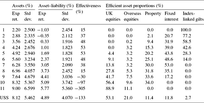
Table 2 shows the risk and return of both the asset and the asset–liability portfolios, as well as the investment proportions themselves, for a range of points on the efficient frontier. The asset–liability portfolios use the USS funding ratio of 101%. For low risk portfolios, the size of the optimal holding by USS of index linked gilts represents a substantial proportion of the market. This can be overcome by using the index linked swaps market, or by placing constraints on the maximum holding of index linked gilts. The last line of Table 2 shows the actual USS asset allocation on 31 January 2002. This portfolio is plotted in Figure 1 as USSa (USS assets only) and USSal (USS assets and liabilities). The efficient frontiers for these two alternative sets of portfolios are plotted in Figure 1. While the asset–liability quadratic programming model must generate convex efficient sets, the assets-only frontier may not necessarily be convex. Table 2 and Figure 1 show that the asset–liability numbers have lower risk and lower return than the corresponding asset-only numbers, highlighting the fact that the model allows the pension scheme to hedge the liability risk.

The USS Statement of Investment Principles (SIP) supports the objective of “funding the scheme’s benefits at the lowest cost over the long term, having regard to the minimum funding requirement of the Pensions Act 1995 and having regard to the attitude of the Committee of Vice-Chancellors and Principals and of the Management Committee towards the risk of higher contributions at some time in the future”, Universities Superannuation Scheme (2002). Given these objectives, the relevant values for decision taking by the pension scheme are those reflecting its net position, rather than the unhedged, or gross, asset returns and risks. The scheme is taking positions on the spread between investment returns and the rate of increase in retail prices and salaries. Thus, while small changes in the difference between these two returns may be important for the pension scheme, big changes in both may not. The asset–liability efficient frontier can be viewed as the outcome of a risk-minimizing generalized hedge, subject to the constraints of a given rate of return and a hedge ratio of (![]() ) or −0.9918747.
) or −0.9918747.
Table 2 also shows the Ederington (1979) measure of hedging effectiveness, which gives the reduction in the variance of the asset–liability portfolio, relative to the variance of the fund’s liabilities. This shows that the best hedge occurs for portfolios 4 and 5, which offer a 50% reduction in risk. It also shows that for portfolios 9 to 11 (and USS), the risk of the hedged portfolio exceeds that of the liabilities alone, so that the fund faces additional asset risk in addition to the basic risk of its liabilities.
The expected return for portfolios 1 and 2 for the assets and liabilities together is negative; a fact obscured if only the asset returns are considered. The results also demonstrate the interaction between assets and liabilities in the model, as the asset–liability frontier is not simply a linear transformation of the assets-only frontier (e.g., each point on the asset frontier shifted the same distance to the south west). For example, the risk-minimizing portfolio for the asset–liability model is portfolio 4, while for the assets-only portfolio it is portfolio 2. The expected return on the assets in the risk-minimizing portfolio 4 is 4.24%, which compares with a discount rate of 5.5% used in computing the actuarial liabilities. Thus, the asset–liability results reveal that portfolios 1, 2 and 3 are dominated, while the assets-only numbers incorrectly suggest that only portfolio 1 is dominated. Similarly, the slopes of the efficient frontiers differ, and the correct risk-return trade-off facing the pension scheme for any specified rate of return (or risk) is that provided by the asset–liability results, not the assets-only results. This confirms the view that any pension scheme should adopt an asset–liability based analysis of the asset allocation, rather than attempting to consider the asset allocation separately from the liabilities.
10 Transformation of the portfolio returns to contribution rates and funding ratios
As noted in Section 3, pension scheme trustees usually prefer to judge the results from portfolio models in terms of the implied level and dispersion of the contribution rate and funding ratio, rather than the risk and return of the asset or asset–liability allocation. For example, the declared objectives of USS can be summarized as simultaneously minimizing the average contribution rate and the variance of the contribution rate. The academic literature has considered three main objectives: (a) minimize the expected contribution rate, (b) minimize the variance of the contribution rate, and (c) minimize the variance of the funding ratio. USS takes the view that the first two objectives are the most important criteria for a well-funded scheme where insolvency is very unlikely. For the generalized Haberman model with a fixed spread period, the variance of the contribution rate is a linear function of the variance of the funding ratio, and so the choice between these two measures of risk is of little consequence. However, for regulatory reasons, the distribution of the funding ratio will also be considered, to ensure that the asset allocation decision is unlikely to lead to any regulatory problems.
In 2002 USS had a funding ratio of 101% and set the employers’ contribution rate for the next three years at 14%, the same rate as in the preceding six years. This suggests that USS was in a fairly stable position, which is consistent with the Haberman (1992) model’s requirement that the pension scheme is in long run equilibrium.
Eqs. (17)-(20) were used to calculate the mean and variance of the contribution rate and funding ratio of each efficient portfolio for both the Haberman (1992) and generalized Haberman models. For the generalized Haberman model the only additional parameters are M and d, while for the Haberman (1992) model many more parameters are required to re-compute the three actuarial liabilities. These parameters were based on Universities Superannuation Scheme (2003). The USS actuary used one rate for computing the standard contribution rate (i.e., a nominal yield of 6%) and a different rate for computing the funding ratio of the scheme, and hence the contribution rate adjustment (i.e., a current yield of 5%). The values of ![]() and
and ![]() were used.
were used.
The results for the Haberman (1992) model and the actual USS portfolio on 31 January 2002 are in Table 3. The fund’s objective is assumed to be to minimize both the contribution rate and the standard deviation of the contribution rate, so that for the Haberman (1992) model portfolios to the north east of the minimum contribution rate risk portfolio (i.e., portfolios 1 to 6 in Table 2) are mean-variance dominated and need not be considered further. Thus, the transformation from the mean and variance of portfolio returns to the mean and variance of the contribution rate results in the exclusion of portfolios 4 to 6 from further consideration. This is in addition to portfolios 1 to 3, which were found to be dominated using asset–liability returns, see Table 5. The funding ratio for the Haberman (1992) model (FR) is constrained to be 100%, and the USS portfolios have been converted to the same basis. If the funding ratio is computed using a fixed discount rate of 5.5% (as in the generalized Haberman model), it ceases to be 100%.
Table 3 The first two moments of the contribution rate and funding ratio—Haberman (1992) model with M=12

Table 4 and Figure 2 show that, for the generalized Haberman model, the lowest contribution rate risk occurs for portfolios 2 and 3, while portfolio 3 has the lowest funding ratio risk. So, in this case, only portfolio 1 is dominated. Table 5 indicates that, while portfolios 2 and 3 are dominated when using asset–liability returns, they are not dominated when the generalized Haberman model is used. The generalized Haberman model allows FR to depart from 100%, as shown in Table 4. (The USS plots in Figures 2 and 3 use the funding ratio of 101%.) For portfolios 1–5, the funding ratio is below 100% because, although the contribution rate is high, the expected return on assets is low.
Table 4 The first two moments of the contribution rate and funding ratio—generalized Haberman model with M=12

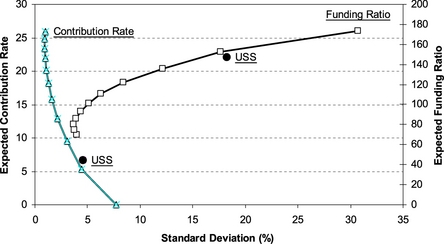
Table 5 Mean-variance dominance
| Model | Dominated portfolios |
| Assets only portfolios | 1 |
| Asset–liability portfolios | 1, 2, 3 |
| Contribution rates for Haberman (1992) with M=12 | 1, 2, 3, 4, 5, 6 |
| Contribution rates for generalized Haberman with M=12 | 1 |

Figure 3 shows the trade-off between the contribution rate and the standard deviation of the funding ratio. Figure 3 reveals that, for the generalized Haberman model with a fixed spread period, there is a positive linear relationship between the standard deviations of the contribution rate and the funding ratio. This is in sharp contrast to the convex relationship for the Haberman (1992) model, which is also shown in Figure 3. The efficient set for the Haberman (1992) model in Figure 3 is the curve AB (portfolios 7 to 11).
11 Choice of the spread period
In Section 10, the spread period, M, was set to the value used by USS (12 years). However, it is possible that a different choice of M would improve the risk-return performance of the scheme. Section 5 described the estimation of ![]() , the spread period which minimizes the contribution rate.
, the spread period which minimizes the contribution rate. ![]() cannot be computed when the rate of salary growth exceeds the expected rate of return on the assets (because
cannot be computed when the rate of salary growth exceeds the expected rate of return on the assets (because ![]() is then negative), which is the case for the low return portfolios 1, 2 and 3. As Table 6 shows, for the Haberman (1992) model these are dominated portfolios, and so this is not a significant issue. However, for the generalized Haberman model Table 7 shows that this condition rules out portfolios 1 to 6, of which only the first is dominated.
is then negative), which is the case for the low return portfolios 1, 2 and 3. As Table 6 shows, for the Haberman (1992) model these are dominated portfolios, and so this is not a significant issue. However, for the generalized Haberman model Table 7 shows that this condition rules out portfolios 1 to 6, of which only the first is dominated.
Table 6 The first two moments of the contribution rate and funding ratio—Haberman (1992) model with ![]()
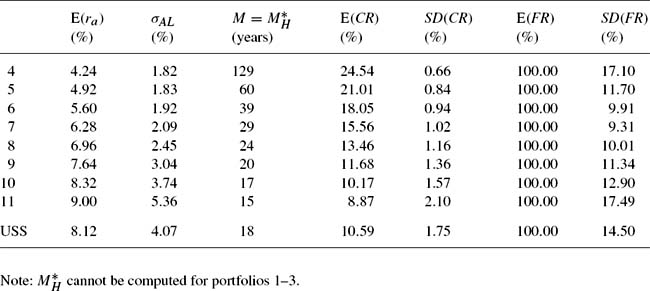
Table 7 The first two moments of the contribution rate and funding ratio—generalized Haberman model with ![]()
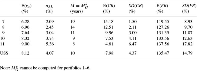
Tables 6 and 7 show the optimal spread period for each portfolio (including the USS portfolio on 31 January 2002) for the Haberman (1992) and generalized Haberman models. For the Haberman (1992) model the fund’s chosen spread period of 12 years is always less than the optimal spread period. As discussed in Section 5, for the Haberman (1992) model using a spread period shorter than ![]() reduces
reduces ![]() , but increases
, but increases ![]() . Therefore, although
. Therefore, although ![]() can be reduced by lowering the spread period, this comes at the expense of an increase in
can be reduced by lowering the spread period, this comes at the expense of an increase in ![]() . Since the two principal objectives used in this paper are to minimize both the mean and variance of the contribution rate, the possibility of minimizing
. Since the two principal objectives used in this paper are to minimize both the mean and variance of the contribution rate, the possibility of minimizing ![]() is not pursued. For the generalized Haberman model, both
is not pursued. For the generalized Haberman model, both ![]() and
and ![]() rose as
rose as ![]() fell.
fell.
The transformation of the portfolio results into the mean and variance of the contribution rate and funding ratio in the previous section was repeated using the relevant value of ![]() (rounded to the nearest integer) from Tables 6 and 7. As can be seen by comparing Tables 3 and 6 for the Haberman (1992) model, the use of
(rounded to the nearest integer) from Tables 6 and 7. As can be seen by comparing Tables 3 and 6 for the Haberman (1992) model, the use of ![]() in place of the fund’s standard spread period of 12 years, increases
in place of the fund’s standard spread period of 12 years, increases ![]() in every case, sometimes by substantial amounts. However, as expected, there were reductions in
in every case, sometimes by substantial amounts. However, as expected, there were reductions in ![]() . A comparison of Tables 4 and 7 reveals that, for the generalized Haberman model, moving to
. A comparison of Tables 4 and 7 reveals that, for the generalized Haberman model, moving to ![]() leads to a reduction in
leads to a reduction in ![]() , with the size of the reduction depending on the size of the change in M. There is no reduction in
, with the size of the reduction depending on the size of the change in M. There is no reduction in ![]() for portfolio 8 due to the rounding of the spread period and the insensitivity of
for portfolio 8 due to the rounding of the spread period and the insensitivity of ![]() to M. For portfolios 7 and 8
to M. For portfolios 7 and 8 ![]() , and the values of
, and the values of ![]() rise; while for portfolios 9 to 11 and USS,
rise; while for portfolios 9 to 11 and USS, ![]() and the values of
and the values of ![]() fall. This shows that, when the spread period is not fixed, the trade-off between
fall. This shows that, when the spread period is not fixed, the trade-off between ![]() and
and ![]() reappears.
reappears.
The relationship between ![]() and M is illustrated in Figure 4 for portfolios 7 and 11 using the generalized Haberman model. This shows that for portfolio 7, increasing M from 12 to 19 years reduces
and M is illustrated in Figure 4 for portfolios 7 and 11 using the generalized Haberman model. This shows that for portfolio 7, increasing M from 12 to 19 years reduces ![]() from 1.57% to 1.50%; while for portfolio 11, reducing M from 12 to 8 years reduces this risk from 7.69% to 6.47%. Figure 4 also reveals that, over the relevant range,
from 1.57% to 1.50%; while for portfolio 11, reducing M from 12 to 8 years reduces this risk from 7.69% to 6.47%. Figure 4 also reveals that, over the relevant range, ![]() is not very sensitive to M.
is not very sensitive to M.

12 Allowance for triennial valuations
Both the Haberman (1992) and the generalized Haberman models assume annual actuarial valuations. However, most schemes have triennial actuarial valuations. The effects of triennial valuations on the variances of the contribution rate and the funding ratio were investigated by comparing the Dufresne (1988) and Haberman (1993b) models, which are summarized in Appendix A. Triennial valuations may increase or decrease the variance of the contribution rate, see Haberman (1993b) and Cairns (1996a). The Dufresne (1988) model is similar to the Haberman (1992) model, except that there is no lag in adjusting the contribution rate, and differs from the Haberman (1993b) only in that the latter assumes triennial actuarial valuations. Therefore a comparison of the results from these two models will reveal the increase in the variances caused by the introduction of triennial valuations. Using the USS data described above, but with M set equal to the value of ![]() for the model concerned, it was found that the understatement of the variances of CR and FR due to the absence of a one year lag was only about 2.6% (or 2.7% when
for the model concerned, it was found that the understatement of the variances of CR and FR due to the absence of a one year lag was only about 2.6% (or 2.7% when ![]() years). This suggests that a move to triennial valuations would make little difference to the variances of CR and FR, or to the other results in this chapter.
years). This suggests that a move to triennial valuations would make little difference to the variances of CR and FR, or to the other results in this chapter.
Even if there had been a material effect on the variances by switching to triennial valuations, a model which assumes annual valuations may still be preferable. This is because many pension schemes, including USS, make an annual actuarial check on the funding ratio, after which the contribution rate could be adjusted. This is effectively an annual review of the contribution rate, even though a full actuarial valuation is performed only every three years.
13 Regulatory and solvency risk
In order to investigate solvency risk, a knowledge of the probability distribution of the funding ratio is required. The parameters of the distribution of the funding ratio were computed using the equations in Section 6 for the generalized Haberman model with ![]() and
and ![]() . The inverted gamma distribution was then used to compute the values of the shortfall probability (SP) and the ETL for the upper and lower regulatory restrictions. The values of SP and ETL were for one year. To obtain results for say a 3-year period, assuming that proportionate changes in the funding ratio are independent over time, the mean and variance of the FR used in Eqs. (23) and (24) must be multiplied by 3. If proportionate changes in the FR are correlated, a more complicated adjustment is required (Jorion, 2000).
. The inverted gamma distribution was then used to compute the values of the shortfall probability (SP) and the ETL for the upper and lower regulatory restrictions. The values of SP and ETL were for one year. To obtain results for say a 3-year period, assuming that proportionate changes in the funding ratio are independent over time, the mean and variance of the FR used in Eqs. (23) and (24) must be multiplied by 3. If proportionate changes in the FR are correlated, a more complicated adjustment is required (Jorion, 2000).
As a simple approximation to the lower solvency bound that will apply after the abolition of the MFR, the specified VaR for the lower tail was set at 70%, which roughly approximates to 100% MFR funding. While the MFR funding ratio is due to be replaced by scheme-specific funding requirements (Secretary of State for Work and Pensions, 2002), it was decided to use the current MFR as the lower bound. Because each of the regulatory restrictions requires the use of a valuation basis that differs from that used to determine the contribution rate, the funding ratios of 90% and 105% were adjusted to be comparable with those used elsewhere in this paper. At the 2002 actuarial valuation the MFR funding ratio for USS was 144%, as against a funding ratio of 101% using the assumptions of the USS actuary. This implies a lower solvency bound of ![]() . The upper bound, imposed to prevent over-funding, was set at
. The upper bound, imposed to prevent over-funding, was set at ![]() .
.
The results are in Tables 8 and 9. The ETLs in Tables 8 and 9 were computed by setting m, the number of samples, to 100. When ![]() ,
, ![]() drops to zero for portfolios 4–11, while for portfolio 1 it is over 50%. This reflects the negative expected asset returns for portfolios 1 and 2, and the larger expected returns for higher numbered portfolios. Conversely, for portfolios 1–7,
drops to zero for portfolios 4–11, while for portfolio 1 it is over 50%. This reflects the negative expected asset returns for portfolios 1 and 2, and the larger expected returns for higher numbered portfolios. Conversely, for portfolios 1–7, ![]() , but as the expected asset return and risk rise,
, but as the expected asset return and risk rise, ![]() rises to over 85% for
rises to over 85% for ![]() . Even though portfolio 1 has a 50% chance of breaching the MFR when
. Even though portfolio 1 has a 50% chance of breaching the MFR when ![]() , the expected value of the funding ratio (ETL) is still 67%, i.e. a 3% breach. Portfolio 11 has an 85% probability of breaching the upper bound when
, the expected value of the funding ratio (ETL) is still 67%, i.e. a 3% breach. Portfolio 11 has an 85% probability of breaching the upper bound when ![]() , and the expected funding ratio is 180%, i.e., a breach of 37%. Thus, the average breach of the upper bound tends to be much bigger than the average breach of the lower bound, reflecting the strong positive skewness of the distribution of the funding ratio.
, and the expected funding ratio is 180%, i.e., a breach of 37%. Thus, the average breach of the upper bound tends to be much bigger than the average breach of the lower bound, reflecting the strong positive skewness of the distribution of the funding ratio.
Table 8 Solvency and regulatory risk: Shortfall probabilities and ETLs: Generalized Haberman model with M=12
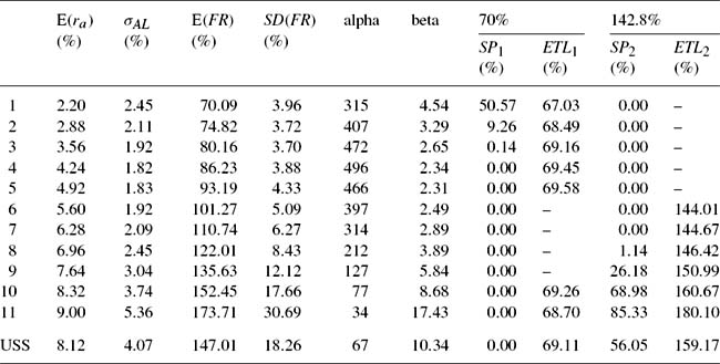
Table 9 Solvency and regulatory risk: Shortfall probabilities and ETLs: Generalized Haberman model with ![]()
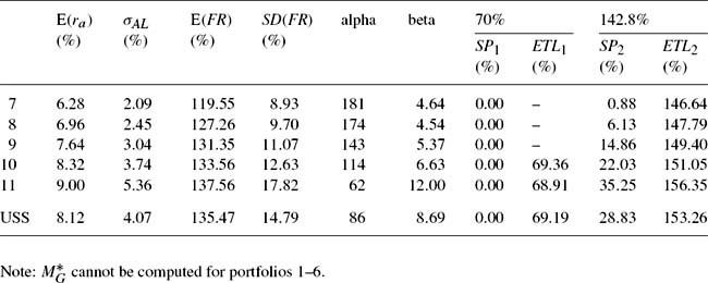
When ![]() , Table 9 shows that the values of
, Table 9 shows that the values of ![]() and
and ![]() are little changed, while for
are little changed, while for ![]() and
and ![]() the values become more even across the range, with falls for high risk and high return portfolios, and rises for lower risk and lower return portfolios. Note that for
the values become more even across the range, with falls for high risk and high return portfolios, and rises for lower risk and lower return portfolios. Note that for ![]() , the values of
, the values of ![]() and
and ![]() for portfolios 7 and 8 are larger than when
for portfolios 7 and 8 are larger than when ![]() ; while for portfolios 9–11, the reverse is the case. This is because
; while for portfolios 9–11, the reverse is the case. This is because ![]() for portfolios 7 and 8, and any surplus is removed more slowly, permitting high funding ratios to be attained; while for portfolios 9–11,
for portfolios 7 and 8, and any surplus is removed more slowly, permitting high funding ratios to be attained; while for portfolios 9–11, ![]() , and any surplus is eliminated more quickly.
, and any surplus is eliminated more quickly.
14 Conclusions
This paper had modeled a number of aspects of pension trustees’ decisions concerning the asset allocation and contribution rate. A simple extension of the portfolio model permits the inclusion of different types of liability in the computation of the efficient asset proportions for various levels of risk and return. Pension schemes generally state that their asset allocation decision has taken account of their liabilities. However, they have usually not explicitly incorporated the liabilities into the asset allocation decision. The asset allocations derived from this extended model are different from those derived from an assets-only formulation, and offer significant hedging of the schemes’ liabilities. Because of this, it is important that the results of the portfolio analysis are presented to decision makers in terms of the risks and returns on the combination of the assets and liabilities of the scheme, rather than just the assets alone.
An analysis of the asset allocation decision in terms of its effects on the risks and returns of the assets and liabilities of the scheme does not explicitly consider the effects on the contribution rate and the funding ratio. This paper shows how the results of a portfolio model can be re-expressed in terms of the first two moments of the contribution rate and funding ratio. By presenting decision makers with the implications of alternative asset allocations for the mean and variance of the contribution rate and funding ratio, the problem is translated into the variables which ultimately concern the trustees. This transformation can also reveal additional or reduced mean-variance dominance between alternative asset allocations.
Computing the effects of the asset allocation decision on the contribution rate, enables the actuary to calculate the spread period which minimizes contribution rate risk for the chosen asset allocation. This paper generalizes the Haberman (1992) model by dropping the requirement that the discount rate equals the rate of return on the investments. As well as improving the economic realism of the model, this greatly simplifies its empirical application because the actuarial valuation need not be repeated for a range of different discount rates. In addition, it removes the trade-off between contribution rate risk and funding ratio risk (for a fixed spread period). The Haberman (1992) model and the generalized Haberman model were applied to data for the Universities Superannuation Scheme, and the efficient frontiers plotted for both fixed and optimized spread periods. The trustees then choose a particular combination of the contribution rate and contribution rate risk, which determines the asset allocation.
Finally, the distribution of the funding ratio was considered, in conjunction with the upper and lower statutory limits. This allows trustees to investigate the regulatory and solvency risks associated with a particular asset allocation/contribution rate choice.
The application of the model proposed in this paper requires a change in the way pensions schemes operate. Currently, the contribution rate is usually recommended by the scheme actuary on the basis of an assumed asset allocation; while the actual asset allocation is set separately on the basis of investment advice. The proposed model requires a joint decision by a single person or group, probably at the time the contribution rate is set. The results for USS suggest that this can lead to superior decisions.
Acknowledgements
The authors wish to thank Shirin Hashemi (University of Southampton) for help in deriving equation (22G), Stephen Court (AUT) for supplying the data on academic salaries, Mike Orszag (Watson Wyatt LLP) and Craig Gillespie (Watson Wyatt LLP), Bill Ziemba (University of British Columbia), Peter Casson (University of Southampton) and participants in the Inquire UK, Inquire Europe and Q Group meeting in Versailles, and seminars at the ICMA Centre, Reading, and Watson Wyatt, Reigate for comments on an earlier draft. Although one of the authors is a director of USS Ltd, this paper represents independent research conducted using publicly available information. The views expressed in this paper are those of the authors, and may not be shared by USS.
Appendix A
A.1 Annual actuarial valuations and instant adjustment of the contribution rate (Dufresne, 1988)
A.2 Triennial actuarial valuations and instant adjustment of the contribution rate (Haberman, 1993b)
 (A.10)
References
Accounting Standards Board. Statement of Standard Accounting Practice 24—Accounting for Pension Costs. London: ASB Publications; 1988. May
Accounting Standards Board. Financial Reporting Standard 17—Retirement Benefits. London: ASB Publications; 2000. November
Actuarial Education Company. ActEd Study Materials: 2002 Examinations, Subject 304, Course Notes. Oxford: Actuarial Education Company; 2002.
P. Artzner, F. Delbaen, J.M. Eber, D. Heath. Coherent measures of risk. Mathematical Finance. 1999;9(3):203-228. July
Association of Consulting Actuaries. Occupational Pensions 2003—Pensions Reform: Too Little, Too Late?. ACA; 2003. March
W. Bagehot. Risk and reward in corporate pension funds. Financial Analysts Journal. 1972;28(1):80-84. January–February
D. Bédard. Stochastic Pension funding: Proportional control and bilinear processes. ASTIN Bulletin. 1999;29(2):271-293. November
D. Bédard, D. Dufresne. Pension funding with moving average rates of return. Scandinavian Actuarial Journal. 2001;2001(1):1-17. March
F. Black. The plan sponsor’s goal. Financial Analysts Journal. 1995;51(4):6-7. July–August
D. Blake, B.N. Lehmann, A. Timmermann. Asset allocation dynamics and pension fund performance. Journal of Business. 1999;72(4):429-461. October
J.L.G. Board, C.M.S. Sutcliffe. Estimation methods in portfolio selection and the effectiveness of short sales restrictions: UK evidence. Management Science. 1994;40(4):516-534. April
C.G.E. Boender. A hybrid simulation–optimization scenario model for asset–liability management. European Journal of Operations Research. 1997;99(1):126-135. May
C.G.E. Boender, C.L. Dert, H. Hoek. ALM for pension funds. In: S.A. Zenios, W.T. Ziemba, editors. Handbook of Asset and Liability Management. Elsevier Science, 2006.
C.G.E. Boender, P.C. Van Aalst, F. Heemskerk. Modelling and management of assets and liabilities of pension plans in the Netherlands. In: W.T. Ziemba, J.M. Mulvey, editors. Worldwide Asset and Liability Modelling. Cambridge University Press; 1998:561-580.
Boender, C.G.E., Vos, M., 2000. Risk return budgeting at pension plans. The Institutional Investor, pp. 80–88, May
E. Bogentoft, H.E. Romeijn, S. Uryasev. Asset–liability management for pension funds using CVaR constraints. Journal of Risk Finance. 2001;3(1):57-71. Fall
P. Booth, R. Chadburn, D. Cooper, S. Haberman, D. James. Modern Actuarial Theory and Practice. Boca Raton, FL: Chapman and Hall/CRC; 1999. Chapter 25
Boulier, J.F., Michel, S., Wisnia, V., 1996. Optimizing investment and contribution policies of a defined benefit pension fund. In: Albrecht, P. (Ed.), Proceedings of the 6th AFIR International Colloquium, Nuremberg, 1996, pp. 593–607
Boulier, J.F., Trussant, E., Florens, D., 1995. A dynamic model for pension funds management. In: Janssen, J. (Ed.), Proceedings of the 5th AFIR International Colloquium, Brussels, 1995, pp. 361–384
G.P. Brinson, L.R. Hood, G.L. Beebower. Determinants of portfolio performance. Financial Analysts Journal. 1986;42(4):39-44. July–August
G.P. Brinson, B.D. Singer, G.L. Beebower. Determinants of portfolio performance II: An update. Financial Analysts Journal. 1991;47(3):40-48. May–June
Cairns, A.J.G., 1995. Pension funding in a stochastic environment: The role of objectives in selecting an asset allocation strategy. In: Janssen, J. (Ed.), Proceedings of the 5th AFIR International Colloquium, Brussels 1995, pp. 429–453
Cairns, A.J.G., 1996a. An introduction to stochastic pension fund management, Working Paper 9607. Pensions Institute
Cairns, A.J.G., 1996b. Continuous time pension fund modelling. In: P. Albrecht (Ed.), Proceedings of the 6th AFIR International Colloquium, Nuremberg, 1996, pp. 609–624
Cairns, A.J.G., 1997. A comparison of optimal and dynamic control strategies for continuous time pension plan models. In: Proceedings of the 7th AFIR International Colloquium, Cairns, 1997, pp. 309–326
A.J.G. Cairns. Some notes on the dynamics and optimal control of stochastic pension fund models in continuous time. ASTIN Bulletin. 2000;30(1):19-55. May
A.J.G. Cairns, G. Parker. Stochastic pension fund modelling. Insurance: Mathematics and Economics. 1997;21(1):43-79. October
J.Y. Campbell, L.M. Viceira. Strategic Asset Allocation: Portfolio Choice for Long Term Investors. Oxford University Press; 2002.
D.R. Cariño, W.T. Ziemba. Formulation of the Russell–Yasuda Kasai financial planning model. Operations Research. 1998;46(4):433-449. July–August
D.R. Cariño, D.H. Myers, W.T. Ziemba. Concepts, technical issues and uses of the Russell–Yasuda Kasai financial planning model. Operations Research. 1998;46(4):450-462. July–August
D.R. Cariño, T. Kent, D.H. Myers, C. Stacy, M. Sylvanus, A.L. Turner, K. Watanabe, W.T. Ziemba. The Russell–Yasuda Kasai model: An asset–liability model for a Japanese Insurance Company using multistage stochastic programming. Interfaces. 1994;24(1):29-49. January–February
S.C. Chang, C.C. Chen. Allocating unfunded liability in pension valuation under uncertainty. Insurance: Mathematics and Economics. 2002;30(3):371-387. June
V.K. Chopra, W.T. Ziemba. The effect of errors in means, variances and covariances on optimal portfolio choice. Journal of Portfolio Management. 1993;19(2):6-11. Winter
G.M. Constantinides. Rational asset prices. Journal of Finance. 2002;57(4):1567-1591. August
B. Cornell. The Equity Risk Premium: The Long-Run Future of the Stock Market. John Wiley and Sons; 1999.
T.M. Craft. The role of private and public real estate in pension plan portfolio allocation choices. Journal of Real Estate Portfolio Management. 2001;7(1):17-23. January–March
T.M. Craft. How funding ratios affect pension plan allocations. Journal of Real Estate Portfolio Management. 2005;11(1):29-35. January–April
G.H. Chun, B.A. Chiochetti, J.D. Shilling. Pension plan real estate investment in an asset–liability framework. Real Estate Economics. 2000;28(3):467-491. Fall
C.L. Dert. A dynamic model for asset liability management for defined benefit pension funds. In: W.T. Ziemba, J.M. Mulvey, editors. Worldwide Asset and Liability Modelling. Cambridge University Press; 1998:501-536.
E. Dimson, P. Marsh, M. Staunton. The Triumph of the Optimists: 101 Years of Global Investment Returns. Princeton University Press; 2002.
G. Dondi, F. Herzog, L. Schuman, H.P. Geering. Dynamic asset and liability management for Swiss pension funds. In: S.A. Zenios, W.T. Ziemba, editors. Handbook of Asset and Liability Management. Elsevier Science, 2006.
K. Dowd. An Introduction to Market Risk Measurement. John Wiley; 2002.
Drijver, S.J., Klein Haneveld, W.K., Van Der Vlerk, M.H., 2002. ALM model for pension funds: Numerical results for a prototype model, Research Report. University of Grongingen
S.J. Drijver, W.K. Klein Haneveld, M.H. Van Der Vlerk. Asset liability management modelling using multi-stage mixed integer stochastic programming. In: B. Scherer, editor. Asset and Liability Management Tools: A Handbook for Best Practice. Risk Books; 2003:309-324.
D. Dufresne. Pension funding and random rates of return. In: M. Goovaerts, F. De Vylder, J. Haezendonck, editors. Insurance and Risk Theory. D. Reidel Publishing; 1986:277-291.
D. Dufresne. Moments of Pension contributions and fund levels when rates of return are random. Journal of the Institute of Actuaries. 1988;115(3):535-544. September
D. Dufresne. Stability of pension systems when rates of return are random. Insurance: Mathematics and Economics. 1989;8(1):71-76. March
Dufresne, D., 1990a. Fluctuations of pension contributions and fund level. Actuarial Research Clearing House, pp. 111–120
D. Dufresne. The Distribution of a perpetuity with applications to risk theory and pension funding. Scandinavian Actuarial Journal (1–2), 1990:39-79.
L.H. Ederington. The hedging performance of the new futures markets. Journal of Finance. 1979;34(1):157-170. March
M. Evans, N. Hastings, B. Peacock. Statistical Distributions, second ed. John Wiley and Sons; 1993. Chapter 18—Gamma distributions
C.J. Exley, S.J.B. Mehta, A.D. Smith. The financial theory of defined benefit pension schemes. British Actuarial Journal. 1997;3:835-966. Part 4
D.D. Ezra. Asset allocation by surplus optimization. Financial Analysts Journal. 1991;47(1):51-57. January–February
F.J. Fabozzi, S.M. Focardi, C.L. Jonas. Market experience with modelling for defined benefit pension funds: Evidence from four countries. Journal of Pension Economics and Finance. 2005;4(3):313-327. November
Faculty and Institute of Actuaries. Pensions and other Benefits, Subject 304 Core Reading, GN26: Pension Fund Terminology. Oxford: Faculty and Institute of Actuaries; 2003.
G.M. Frankfurter, J.M. Hill. A normative approach to pension fund management. Journal of Financial and Quantitative Analysis. 1981;16(4):533-558. November
R. Gerrard, S. Haberman. Stability of pension systems when gains–losses are amortized and rates of return are autoregressive. Insurance: Mathematics and Economics. 1996;18(1):59-71. May
Geyer, A., Herold, W., Kontriner, K., Ziemba, W.T., 2005. The Innovest Austrian Pension Fund financial planning model InnoALM, Working paper. University of British Columbia, February
J. Gondzio, R. Kouwenberg. High performance computing for asset–liability management. Operations Research. 2001;49(6):879-891. November–December
Haberman, S., 1990a. Stochastic approach to pension funding methods. In: Proceedings of the 1st AFIR International Colloquium, Paris, 1990, pp. 93–112
Haberman S., 1990b. Variability of pension contributions and fund levels with random and autoregressive rates of return. Actuarial Research Clearing House, pp. 141–171
S. Haberman. Pension funding with time delays: A stochastic approach. Insurance: Mathematics and Economics. 1992;11(3):179-189. October
S. Haberman. Pension funding with time delays and autoregressive rates of investment return. Insurance: Mathematics and Economics. 1993;13(1):45-56. September
S. Haberman. Pension funding: The effect of changing the frequency of valuations. Insurance: Mathematics and Economics. 1993;13(3):263-270. December
S. Haberman. Autoregressive rates of return and the variability of pension contributions and fund levels for a defined benefit pension scheme. Insurance: Mathematics and Economics. 1994;14(3):219-240. July
Haberman, S., 1994b. Defined benefit pension funding models and stochastic investment returns. Paper presented to a joint meeting of the Staple Inn Actuarial Society and the Royal Statistical Society, March, 50 p
S. Haberman. Pension funding with time delays and the optimal spread period. ASTIN Bulletin. 1995;25(2):177-187. November
S. Haberman. Stochastic investment returns and contribution rate risk in a defined benefit pension scheme. Insurance: Mathematics and Economics. 1997;19(2):127-139. April
S. Haberman. Risk in a defined benefit pension scheme. Singapore International Insurance and Actuarial Journal. 1997;1:93-103.
Haberman, S., 1998. Stochastic modelling of pension scheme dynamics, Actuarial Research Report, No. 106, February, 35 p
S. Haberman, Z. Butt, C. Megaloudi. Contribution and solvency risk in a defined benefit pension scheme. Insurance: Mathematics and Economics. 2000;27(2):237-259. October
S. Haberman, D. Dufresne. Variability of pension contributions and fund levels with random rates of return. In: J.D. Cummins, R.A. Derrig, editors. Managing the Insolvency Risk of Insurance Companies. Kluwer Academic Press; 1991:133-145.
Haberman, S., Owadally, I., 2001. Modelling defined benefit pension schemes: funding and asset valuation. Paper presented to the International Actuarial Association International Pensions Seminar, Brighton, 36 p
S. Haberman, L.Y.P. Wong. Moving average rates of return and the variability of pension contributions and fund levels for a defined benefit pension scheme. Insurance: Mathematics and Economics. 1997;20(2):115-135. September
Haberman, S., Day, C., Fogarty, D., Khorasanee, Z., McWhirter, M., Nash, N., Ngwira, B., Wright, I.D., Yakoubov, Y., 2003. A stochastic approach to risk management and decision making in defined benefit pension schemes, Paper presented to the Institute of Actuaries, 27th January, 95 p
N. Hakansson. Optimal investment and consumption strategies under risk for a class of utility functions. Econometrica. 1970;38(5):587-607. September
N. Hakansson. On optimal myopic portfolio policies with and without serial correlation of yields. Journal of Business. 1971;44(3):324-334. July
P. Hilli, M. Koivu, T. Pennanen, A. Ranne. A stochastic programming model for asset liability management of a Finnish pension company. Annals of Operations Research. 2005.
R.G. Ibbotson, P.D. Kaplan. Does asset allocation policy explain 40, 90 or 100 percent of performance? Financial Analysts Journal. 2000;56(1):26-33. January–February
N.L. Johnson, S. Kotz, N. Balakrishnan, second ed. Continuous Univariate Distributions, vol. 1. New York: John Wiley and Sons; 1994. Chapter 17—Gamma distributions
R. Josa-Fombellida, J.P. Rincón-Zapatero. Minimization of risks in pension funding by means of contributions and portfolio selection. Insurance: Mathematics and Economics. 2001;29(1):35-45. August
P. Jorion. Value at Risk: The New Benchmark for Managing Financial Risk, second ed. McGraw-Hill; 2000.
J.G. Kallberg, W.T. Ziemba. Mis-specification in portfolio selection problems. In: G. Bämberg, K. Spremann, editors. Risk and Capital. Springer-Verlag; 1984:74-87.
L. Kingsland. Projecting the financial condition of a pension plan using simulation analysis. Journal of Finance. 1982;37(2):577-584. May
R. Kouwenberg. Asset liability management for pension funds: Elements of Dert’s model. In: C. Zopounidis, editor. New Operational Approaches for Financial Modelling. Physica-Verlag; 1997:37-48.
R. Kouwenberg. Scenario generation and stochastic programming models for asset liability management. European Journal of Operations Research. 2001;134(2):279-292. October
M.L. Kusy, W.T. Ziemba. A bank asset and liability management model. Operations Research. 1986;34(3):356-376. May–June
M.L. Leibowitz, L.N. Bader, S. Kogelman. Return Targets and Shortfall Risks: Studies in Strategic Asset Allocation. Irwin Professional Publishing; 1996.
D. Logan. The Birth of a Pension Scheme: A History of the Universities Superannuation Scheme. Liverpool University Press; 1985.
J.D. MacBeth, D.C. Emanuel, C.E. Heatter. An investment strategy for defined benefit plans. Financial Analysts Journal. 1994;50(3):34-41. May–June
P. Mandl, L. Mazurová. Harmonic analysis of pension funding methods. Insurance: Mathematics and Economics. 1996;17(3):203-214.
R.C. Merton. Continuous-Time Finance, Revised ed. Blackwell Publishing; 1992.
R.O. Michaud. The Markowitz optimization enigma: Is ‘optimized’ optimal? Financial Analysts Journal. 1989;45(1):31-42. January–February
J. Mossin. Optimal multiperiod portfolio policies. Journal of Business. 1968;41(2):215-229. April
J.M. Mulvey, G. Gould, C. Morgan. An asset and liability management system for towers Perrin–Tillinghast. Interfaces. 2000;30(1):96-114. January–February
J.M. Mulvey, K.D. Simsek, B. Pauling. A stochastic network approach for integrating pension and corporate financial planning. In: A. Nagurney, editor. Innovations in Financial and Economic Networks. Edward Elgar; 2003:67-83.
J.M. Mulvey, A.E. Thorlacius. The towers Perrin global capital market scenario generation system. In: W.T. Ziemba, J.M. Mulvey, editors. Worldwide Asset and Liability Modelling. Cambridge University Press; 1998:286-312.
J.M. Mulvey, F.J. Fabozzi, W.R. Pauling, K.D. Simsek, Z. Zhang. Modernizing the defined benefit pension system. Journal of Portfolio Management. 2005;31(2):73-82. Winter
Nijman, T., Swinkels, L., 2003. Strategies and tactical allocation to commodities for retirement savings schemes, Discussion paper no. 20, Tilburg University, February
M.I. Owadally, S. Haberman. Pension fund dynamics and gains/losses due to random rates of investment return. North American Actuarial Journal. 1999;3(3):105-117.
Owadally, M.I., Haberman, S., 2000. Efficient amortization of actuarial gains and losses in pension plans. Actuarial Research Clearing House, pp. 275–317
J. Ralfe. Why bonds are right for pension funds. Risk. 2001;14(11):54-55. November
Ralfe, J., Speed, C., Palin, J., 2003. Pensions and capital structure: Why hold equities in the pension fund? Society of Actuaries Symposium on the Great Controversy: Current Pension Actuarial Practice in Light of Financial Economics, Vancouver, June
M. Rudolf, W.T. Ziemba. Intertemporal surplus management. Journal of Economic Dynamics and Control. 2004;28(5):975-990. February
Secretary of State for Work and Pensions, 2002. Simplicity, security and choice: Working and saving for retirement, Green Paper, Cm 5677, December
W.F. Sharpe. Asset allocation. In: J.L. Maginn, D.L. Tuttle, editors. Managing Investment Portfolios: A Dynamic Process. second ed. Warren, Gorham and Lamont; 1990:7.1-7.71. Chapter 7
W.F. Sharpe, L.G. Tint. Liabilities—a new approach. Journal of Portfolio Management. 1990;16(2):5-10. Winter
J.J. Siegel. Stocks for the Long Run, third ed. McGraw-Hill; 2002.
C.M.S. Sutcliffe. The cult of the equity for pension funds: Should it get the boot? Journal of Pension Economics and Finance. 2005;4(1):57-85. March
I. Tepper. Optimal financial strategies for trusteed pension plans. Journal of Financial and Quantitative Analysis. 1974;9(3):357-376. June
P.N. Thornton, A.F. Wilson. A realistic approach to pension funding. Journal of the Institute of Actuaries. 1992;119:229-277.
Universities Superannuation Scheme, 2002. Report and Accounts for the Year Ended 31 March 2002
Universities Superannuation Scheme, 2003. Actuarial Valuation Report as at 31 March 2002, March 2003
M.B. Waring. Liability-relative investing II. Journal of Portfolio Management. 2004;31(1):40-53. Fall
I.D. Wright. Traditional pension fund valuation in a stochastic asset and liability environment. British Actuarial Journal. 1998;4:865-901. Part 4
Yang, T., 2003. Defined benefit pension plan liabilities and international asset allocation, Pension Research Council Working Paper no. 2003-5. University of Pennsylvania
Ziemba, W.T., 2003. The Stochastic Programming Approach to Asset, Liability, and Wealth Management, The Research Foundation of AIMR, Charlottesville, VA
W.T. Ziemba. The Russell Yasuda, InnoALM and Related Models for Pensions, Insurance Companies and High Net Worth Individuals. In: S.A. Zenios, W.T. Ziemba, editors. Handbook of Asset and Liability Management, vol. B. Elsevier Science, 2006.
A. Zimbidis, S. Haberman. Delay, feedback and variability of pension contributions and fund levels. Insurance: Mathematics and Economics. 1993;13(3):271-285. December
1 See Ziemba (2003) for an introduction to the application of multi-period stochastic programming to asset–liability management. Geyer et al. (2005) developed a multi-period stochastic programming model for both defined benefit and defined contribution schemes, which was applied to the Siemens AG Österreich defined contribution scheme. Other papers in related areas include Cariño et al. (1994), Cariño and Ziemba (1998), Cariño, Myers and Ziemba (1998) and Ziemba (2006). Fabozzi, Focardi and Jonas (2005) surveyed 28 pension schemes in the UK, USA, Netherlands and Switzerland with average assets of $16 billion. One third of these schemes used MPSP.
2 Waring (2004) deflated by the liabilities, rather than the assets; and expressed the risk and return of the asset–liability portfolio in terms of the alphas and betas of the capital asset pricing model. Nijman and Swinkels (2003) applied the Sharpe–Tint model, but with the simplification that the importance of the liabilities (k) equals the initial funding ratio.
3 When making this adjustment for the Haberman (1993b) model Q is increased to 3Q because this model deals with three year periods.
4 The rules are specified in the Occupational Pension Schemes (Minimum Funding Requirement and Actuarial Valuations) Regulations 1996; as amended by the Occupational Pension Schemes (Minimum Funding Requirement and Miscellaneous Amendments) Regulations 2002.
5 The valuation basis is specified in the Pension Scheme Surpluses (Valuation) Regulations 1987, Statutory Instrument no. 412.
6 This upper limit will shortly be abolished, as will the MFR.
7 For stochastic programming models, Kusy and Ziemba (1986), Cariño et al. (1994), Cariño and Ziemba (1998), and Cariño, Myers and Ziemba (1998) proposed the use of a convex tail risk measure which leads to a concave utility function that can be modeled using a piecewise linear approximation. This convexity means that shortfalls from target levels are penalized more and more as the shortfall increases.