
Handbook of Asset and Liability Management, Vol. 2, No. suppl (C) • 2007
ISSN: 1872-0978
doi: 10.1016/S1872-0978(06)02016-3
Chapter 16 Integrated Risk Control Using Stochastic Programming ALM Models for Money Management
Abstract
A multistage stochastic programming modeling based approach is developed for asset and liability management for fund managers. Managing a fund of investments in a large pool of possible instruments, such as stocks, requires sophisticated analytical capability both in terms of selecting the pool and also in maintaining the performance of the fund within acceptable levels. Given the uncertainty of the future performance of the underlying stocks, the portfolio must be managed or rebalanced temporally as the market and economic conditions change. Such portfolio rebalancing at various points in time allows the fund manager to manage the riskiness of the fund from both the fund managers and the individual clients viewpoints. In doing so, a fund manager must resort to more-advanced analytical risk-control techniques. I apply a multi-prong risk metric system that is designed for the portfolio to achieve desired performance characteristics. The model incorporates important issues such as market impact costs in trading, fund drawdown, market neutrality, and catastrophic risk, within an integrative framework, modeled via stochastic programming. The model is applied to stock fund management involving a large number of securities and its performance is demonstrated with various strategies for portfolio rebalancing. The integrated dynamic multistage stochastic programming model easily outperforms the standard static mean-variance approach (i.e., the Markowitz model) for portfolio management. Sharpe ratios, percent worst draw downs, recovery periods from drawdown, portfolio rate of returns, etc. are used for performance comparisons.
Keywords
• portfolio optimization • stochastic multistage programming • risk management • integrated risk control • money management
JEL classification
• D81 • G11 • C61
1 Introduction
There is a tremendous growth in the number of individuals who are engaged in money management in the twenty-first century, yet only a few implement disciplined, professional money management strategies. During the stock market bubble of the late 1990s, limiting risk was an afterthought, but given the recent stock market action, more managers are considering more sophisticated approaches to portfolio risk management. Typically, only a few have the ability to view their portfolios from a risk/return integrated perspective. Instead, many individuals take a defensive or reactive view of risk in which risk is measured to avoid losses. What is essential for successful money management is to have an offensive or proactive posture in which risks are actively managed. This paper proposes such an integrated framework for fund management using multistage stochastic programming modeling.
Managing a fund of investments in a large pool of possible instruments (i.e., stocks) requires sophisticated analytical capability both in terms of selecting the pool and also in maintaining the performance of the fund within acceptable levels. Given the uncertainty of the future performance of the underlying stocks, it is imperative that the portfolio of stocks (in the fund) be managed or rebalanced temporally as the market and economic conditions change. Such portfolio rebalancing at various points in time allows the fund manager to control the riskiness of the fund from both the fund managers and the individual clients viewpoints. In doing so, a fund manager must attempt to remove the guesswork based on emotions (or gutt feeling) from the decision making and resort to the more-advanced analytical risk-management techniques.
Reading material on money management is quite abundant—a search on Amazon.com on the Internet returns more than 2100 books. Various professional money management services are also available that offer diverse asset allocation strategies based on common risk and time horizon parameters. These allocations are typically optimized using a static mean-variance framework, following the early work on portfolio optimization by Markowitz (1952, 1987), where a static, deterministic model for trading off portfolio expected return with portfolio variance was proposed. See the chapter by Markowitz and Van Dijk in this volume for a current survey of this approach. Variants of this approach that utilize a mean absolute deviation (MAD) functional, rather than portfolio variance, have been proposed, see, e.g., Konno and Yamazaki (1991) and Konno and Kobayashi (1997).
Asset allocation is the practice of dividing resources among different categories such as stocks, bonds, mutual funds, investment partnerships, real estate, cash equivalents, and private equity. Such models are expected to lessen risk exposure since each asset class has a different correlation to the others; when stocks rise, for example, bonds often fall. At a time when the stock market begins to fall, real estate may begin generating above average returns. Consequently, various allocation styles may be specified for the purposes of, say, preservation of capital, generating income, long-term aggressive growth, or striking a balance between income and growth. However, merely diversifying assets to the prescribed allocation model is not going to alleviate the manager from the need to choose individual issues. Indeed, the asset allocation and the choice of individual securities must occur integratively, consistent with the intended risk specification. A further complication in this case is the need for temporal rebalancing in an effort to bring the portfolio back into balance with the original prescription, or a variation thereof consistent with market evolution and changes in risk preferences.
However, static (myopic) models of portfolio optimization fail to capture two important aspects of portfolio rebalancing: (1) trade-off between short-term and long-term consequences of investment strategy, based on the evolution of stochastic factors, and (2) presence of transactions or market impact costs, taxes, etc. that affect portfolio holdings over time, see Ziemba and Mulvey (1998).
In contrast, a sequential decision theoretic optimization framework for portfolio rebalancing is available via multistage stochastic programming (MSP) modeling. This approach allows modeling various future time periods of portfolio revisions explicitly where stochastic dynamic evolution of random parameters (e.g., security returns) can be incorporated via a so-called scenario tree. Each scenario is a timed-sequence of events through the end of the planning horizon with an associated probability of occurrence. Multistage stochastic programming models have been richly applied in a variety of financial applications; see Kusy and Ziemba (1986) for a bank asset/liability management, Cariño and Ziemba (1998) for an asset/liability management problem of a Japanese insurance company, Mulvey and Vladimirou (1992) for a multiperiod stochastic network model for the purpose of asset allocation, and Golub et al. (1997) for fixed income securities management. For applications of stochastic multistage linear programming with a binomial scenario tree of price uncertainty for financial option pricing, see Edirisinghe, Naik and Uppal (1993), and the extensions in Edirisinghe (2004). This article provides a multistage stochastic programming model that incorporates sequential rebalancing of the portfolio in order to maintain the portfolio performance with respect to a multi-prong risk measurement scheme.
Stochastic programming models have found many applications within asset and liability management (ALM) problems, which are generally of a long term nature. ALM attempts to find the optimal investment strategy under uncertainty in both the asset and liability streams. Simultaneous consideration of assets and liabilities can be very advantageous in terms of increasing returns and reducing risk, especially when they have common risk factors leading to high correlations. ALM-MSP models allow for dynamic portfolio rebalancing while satisfying operational or regulatory restrictions and policy requirements, see, e.g., Holmer and Zenios (1995). Early work on application of stochastic programming for financial planning is by Bradley and Crane (1972) and Ziemba and Vickson (1975). Since 1990, there is an increased momentum in such applications, driven partly by the globalization and innovations in the financial markets, but largely due to tremendous improvement in the solution algorithms and computing hardware advances. See Zenios (1995) and Nielsen and Zenios (1996) for fixed income portfolio management; Cariño et al. (1994), Consigli and Dempster (1998), Høyland (1998), and Mulvey, Gould and Morgan (2000) for insurance companies, Dert (1995) for pension funds, Consiglio, Cocco and Zenios (2001) for minimum guarantee products, as well as Zenios (1993) and Ziemba and Mulvey (1998). Also, see Ziemba (2003) and other chapters in this volume.
I present a stochastic programming model for money management where frequent short-term portfolio rebalancing is commonplace and transactions costs and market impact costs play a significant role in determining trade sizes. Stochastic multiperiod models (of ALM type) are utilized to trade-off returns and transactions costs under various metrics of risk aversion. Indeed, such an approach must be adapted to market evolutionary parameters and optimized for possible errors in parameter forecasts via a specific investment strategy. The model is applied to historical time series of a large stock base and out-of-sample portfolio performance is tracked over daily rollover operation. The main focus is in developing the model and discussing its investment performance, rather than efficient solution algorithms for multistage stochastic programs of this type. The reader interested in the latter aspect is referred to the recent paper by Edirisinghe and Patterson (2007), in which a very efficient solution methodology is developed for real-time solution. Given that high frequency data are readily available on a global basis and computing hardware are becoming more powerful by orders of magnitude, sophisticated modeling techniques as presented here are expected to find broader appeal among the professional investment community.
Section 2 presents an introduction to formulating a multistage stochastic programming (MSP) model. This section also collects the necessary tree notation that will be required for understanding a MSP model. Section 3 provides the basic constructs of the MSP model for the investment optimization problem and several key policy constraints. Section 4 covers various issues with risk metrics and it introduces new and known methodologies for risk control. The multistage stochastic program for trade rebalancing problem is presented in Section 5, and the model application and results analyses are in Section 6. Concluding remarks are in Section 7. The required notation is introduced as it becomes necessary.
2 Multistage stochastic programming (MSP)
Multiperiod stochastic programs can be used to model a sequence of decision-observation processes in which decisions at any point in time are based upon historical observations coupled with beliefs or expectations concerning the uncertainty of future events. The term period is used to refer to the time starting with one decision or set of decisions and lasting until the next decision or set of decisions. See Birge, Edirisinghe and Ziemba (2001) for some applications of stochastic programming models and Birge and Louveaux (1997) for certain terms and definitions concerning stochastic linear programs. For a complete bibliography on stochastic programming, see van der Vlerk (2003).
Decision trees, often referred to as event or scenario trees, are a useful tool for visualizing the resulting model. Decision trees demonstrate the nonanticipative requirement of stochastic programs—decisions in a given period must be made without the hindsight (or the anticipation) of a specific future outcome. The notation used in the development and discussion of multistage stochastic programs is not unique in the literature. The following notation that makes explicit the dependence of decisions and random events on historical scenario paths is used. Assume the number of outcomes ![]() possible at any node in period
possible at any node in period ![]() for arbitrary but finite T is the same for all nodes in that period. There are then
for arbitrary but finite T is the same for all nodes in that period. There are then ![]() total nodes in period t and
total nodes in period t and ![]() cumulative nodes in periods 1 through t. Nodes are labeled using a path vector format. The path vector, say
cumulative nodes in periods 1 through t. Nodes are labeled using a path vector format. The path vector, say ![]() , to a node in period t is a row vector of
, to a node in period t is a row vector of ![]() elements where element j,
elements where element j, ![]() , is the index,
, is the index, ![]() , of the outcome in period j along the path of outcomes to the applicable node. The path to a node in period t is called a t-period scenario and each T-period scenario is usually simply called a scenario of the stochastic program. Let
, of the outcome in period j along the path of outcomes to the applicable node. The path to a node in period t is called a t-period scenario and each T-period scenario is usually simply called a scenario of the stochastic program. Let ![]() represent a t-period scenario, i.e., the (historical) path vector to a node at the beginning of period t, see Figure 1. The single first period root node is labeled using the notation
represent a t-period scenario, i.e., the (historical) path vector to a node at the beginning of period t, see Figure 1. The single first period root node is labeled using the notation ![]() , or simply by
, or simply by ![]() for brevity, which represents the absence of any historical scenario path. By convention,
for brevity, which represents the absence of any historical scenario path. By convention, ![]() and
and ![]() appearing in the same expression implies that the former is the parent node of the latter while
appearing in the same expression implies that the former is the parent node of the latter while ![]() is a child node of
is a child node of ![]() .
.

A decision (vector) taken at node ![]() is denoted by
is denoted by ![]() . It is a nonanticipative decision that depends only on the specific history
. It is a nonanticipative decision that depends only on the specific history ![]() , which corresponds to the sequence of observed outcomes of the random vectors
, which corresponds to the sequence of observed outcomes of the random vectors ![]() , respectively. Having made the decision
, respectively. Having made the decision ![]() , the random vector
, the random vector ![]() will be observed whose domain of realizations are indicated by
will be observed whose domain of realizations are indicated by ![]() , which form the set of child nodes emanating from node
, which form the set of child nodes emanating from node ![]() .
.
The path-vector notation is also used to implicitly indicate the dependence of a stochastic array at a node in period t on the occurrence of the specific outcomes listed by the path vector. Let ![]() represent the period t outcome with index
represent the period t outcome with index ![]() ,
, ![]() , and let
, and let ![]() represent a node in period t,
represent a node in period t, ![]() . Then,
. Then,
represents a conditional stochastic matrix at node ![]() . The conditional probability that the outcome with index
. The conditional probability that the outcome with index ![]() ,
, ![]() ,
, ![]() , is observed at the t-period node
, is observed at the t-period node ![]() given the indicated outcomes
given the indicated outcomes ![]() in periods
in periods ![]() is
is ![]() , i.e.,
, i.e.,
where ![]() is the probability operator and
is the probability operator and ![]() . The joint probability,
. The joint probability, ![]() , that the process enters the period t node
, that the process enters the period t node ![]() ,
, ![]() , is the product of the conditional probabilities of the outcomes along the indicated path to that node,
, is the product of the conditional probabilities of the outcomes along the indicated path to that node,
where ![]() , i.e., the single first period (root) node is always entered.
, i.e., the single first period (root) node is always entered.
2.1 MSP model formulation
Using this notation for decision trees, a multiperiod stochastic program can be formulated recursively by considering the nodal decision problems. A linear stochastic programming model is presented for clarity; extensions to a general nonlinear framework is quite straightforward, see, e.g., formulations in Edirisinghe and Ziemba (1992) and Frauendorfer (1996). The decision process up to (tree) node ![]() has observed the realization sequence indexed as
has observed the realization sequence indexed as ![]() , and corresponds to the decision vector sequence
, and corresponds to the decision vector sequence ![]() . The nodal value function
. The nodal value function ![]() for a period t,
for a period t, ![]() , is the optimal profits to be realized after observing the event indexed by
, is the optimal profits to be realized after observing the event indexed by ![]() and by choosing the decision vector
and by choosing the decision vector ![]() to optimally trade off current profits
to optimally trade off current profits ![]() and the expected value of optimal profits at the child nodes, i.e.,
and the expected value of optimal profits at the child nodes, i.e., ![]() for each of
for each of ![]() . This nodal decision problem is formulated as follows, for
. This nodal decision problem is formulated as follows, for ![]() .
.
![]()
The nodal value function, ![]() , for a node at terminal period T, is
, for a node at terminal period T, is
![]()
Array dimensions are not explicitly listed for reasons of brevity and all arrays are assumed to have shapes and sizes compatible with the depicted operation. Then, the multistage stochastic program can be equivalently represented as the following compact recursive value function formulation.

![]()
3 Investment optimization model
There are N securities that an investor wishes to trade at time ![]() , i.e., at the beginning of period 1. The investor’s initial position (i.e., the number of shares in each security) is
, i.e., at the beginning of period 1. The investor’s initial position (i.e., the number of shares in each security) is ![]() (
(![]() ) and the initial cash position is
) and the initial cash position is ![]() . The price of security j at the first trading node, i.e., the root node
. The price of security j at the first trading node, i.e., the root node ![]() , is $
, is $![]() per share, see Figure 1 for the decision tree. The investor considers trading in multiple periods of time, denoted by the time index
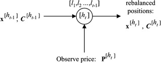
per share, see Figure 1 for the decision tree. The investor considers trading in multiple periods of time, denoted by the time index ![]() . Given the historical price vectors
. Given the historical price vectors ![]() , up until the beginning of trading for period t, the (conditional) rate of return vector for period t is
, up until the beginning of trading for period t, the (conditional) rate of return vector for period t is ![]() . See Figure 2 for an illustration of the nodal trading information. Thus, price of security j changes during the trading period t to
. See Figure 2 for an illustration of the nodal trading information. Thus, price of security j changes during the trading period t to ![]() . Note that
. Note that ![]() since the security prices are nonnegative, i.e.,
since the security prices are nonnegative, i.e., ![]() . Moreover,
. Moreover, ![]() is random and it is observed only at the end of the current period t; however, trade decisions
is random and it is observed only at the end of the current period t; however, trade decisions ![]() must be made at the beginning of period t, i.e., revision of portfolio positions from
must be made at the beginning of period t, i.e., revision of portfolio positions from ![]() to
to ![]() . Therefore,
. Therefore, ![]() is the amount of shares purchased if it is positive; and if it is negative, it is the amount of shares sold in security j. This trade vector is
is the amount of shares purchased if it is positive; and if it is negative, it is the amount of shares sold in security j. This trade vector is ![]() and equals
and equals ![]() where
where ![]() is the absolute value.
is the absolute value.
The investment optimization problem is concerned with determining the trade vectors ![]() such that various risk specifications for the portfolio are met whilst maximizing the portfolio total expected return. Capturing this problem within a multistage framework is advantageous due to at least two important considerations. First, trading (for portfolio rebalancing) is generally not costless. Typically, with larger trade sizes, there is an increasingly diluting effect on the profitability of the trades due to market impact. Thus, it may be beneficial to create an intended position over multiple periods as the trading costs increase. Secondly, due to policy on risk control, portfolio wealth trajectory may have to be monitored, such as the case when portfolio drawdown is an important issue in fund management. Such drawdowns cannot be managed effectively via single period modeling.
such that various risk specifications for the portfolio are met whilst maximizing the portfolio total expected return. Capturing this problem within a multistage framework is advantageous due to at least two important considerations. First, trading (for portfolio rebalancing) is generally not costless. Typically, with larger trade sizes, there is an increasingly diluting effect on the profitability of the trades due to market impact. Thus, it may be beneficial to create an intended position over multiple periods as the trading costs increase. Secondly, due to policy on risk control, portfolio wealth trajectory may have to be monitored, such as the case when portfolio drawdown is an important issue in fund management. Such drawdowns cannot be managed effectively via single period modeling.
3.1 Transactions and slippage costs
Usually, fund managers face transactions costs in executing the trade vector, ![]() , which leads to reducing the portfolio net return. Placing a trade with a broker for execution entails a direct cost per share traded, as well as a fixed cost independent of the trade size. For instance, a $10 fixed cost and a 2-cent per-share cost may be levied. In addition, there is also a significant cost due to the size of trading volume
, which leads to reducing the portfolio net return. Placing a trade with a broker for execution entails a direct cost per share traded, as well as a fixed cost independent of the trade size. For instance, a $10 fixed cost and a 2-cent per-share cost may be levied. In addition, there is also a significant cost due to the size of trading volume ![]() , as well as the broker’s ability to place the trading volume on the market. If a significant volume of shares is traded (relative to the market daily traded volume in the security), then the trade execution price may be adversely affected. A large buy order usually lead to trade execution at a price higher than intended and a large sell order leads to an average execution price that is lower than desired. This dilution of the profits of the trade is termed the market impact loss, or slippage. This slippage loss generally depends on the price at which the trade is desired, trade size relative to the market daily volume in the security, and other company specifics such as market capitalization, and the beta of the security. See Keim and Madhavan (1996, 1997, 1998), Loeb (1983), and Torre and Ferrari (1999), for instance, for a discussion on market impact costs.
, as well as the broker’s ability to place the trading volume on the market. If a significant volume of shares is traded (relative to the market daily traded volume in the security), then the trade execution price may be adversely affected. A large buy order usually lead to trade execution at a price higher than intended and a large sell order leads to an average execution price that is lower than desired. This dilution of the profits of the trade is termed the market impact loss, or slippage. This slippage loss generally depends on the price at which the trade is desired, trade size relative to the market daily volume in the security, and other company specifics such as market capitalization, and the beta of the security. See Keim and Madhavan (1996, 1997, 1998), Loeb (1983), and Torre and Ferrari (1999), for instance, for a discussion on market impact costs.
In our model, a quadratic simplification for the market impact cost is utilized. That is, the slippage costs are proportional to the square of the volume traded in the market, and the constant of proportionality depends directly on the intended execution price, and inversely on the (daily) share volume in that security. For trading ![]() shares of security j (with the intended trade price
shares of security j (with the intended trade price ![]() when the expected total daily volume is
when the expected total daily volume is ![]() shares), thus, leads to a market impact cost of
shares), thus, leads to a market impact cost of

where ![]() is a constant calibrated to the market data. The direct cost of trading is represented by
is a constant calibrated to the market data. The direct cost of trading is represented by ![]() where
where ![]() is the per-share transactions cost. The fixed costs of trading are ignored here, and then, the total transactions and slippage loss function
is the per-share transactions cost. The fixed costs of trading are ignored here, and then, the total transactions and slippage loss function ![]() is
is
 (4)
(4)Therefore, the total loss due to portfolio rebalancing at time t, given the historical scenario ![]() of security price evolution, is
of security price evolution, is
 (5)
(5)3.2 Budget and portfolio wealth
Portfolio rebalancing from period-to-period is assumed to carry forward any cash that is accumulated (i.e., the riskless security) and the total cost of trading at the beginning of period t is thus limited by the cash carried forward from period ![]() , denoted by the nonnegative variable
, denoted by the nonnegative variable ![]() , and any exogenous funds available at the beginning of period t, denoted by
, and any exogenous funds available at the beginning of period t, denoted by ![]() . Then, the following budget constraint must hold.
. Then, the following budget constraint must hold.
The transposition of the price vector ![]() is suppressed for clarity of exposition in the above expression, as well as throughout the remainder of the chapter. When applying the budget constraint (6) for trading at the root node
is suppressed for clarity of exposition in the above expression, as well as throughout the remainder of the chapter. When applying the budget constraint (6) for trading at the root node ![]() , by convention,
, by convention, ![]() , the initial security positions, and
, the initial security positions, and ![]() , the initial cash position. Note that “cash” carried forward yields a deterministic monetary return from period to period given by the rate
, the initial cash position. Note that “cash” carried forward yields a deterministic monetary return from period to period given by the rate ![]() (⩾1), which is already adjusted to the length of the period t. Thus,
(⩾1), which is already adjusted to the length of the period t. Thus, ![]() is the excess cash carried forward and available for portfolio rebalancing at node
is the excess cash carried forward and available for portfolio rebalancing at node ![]() of period
of period ![]() . In the event that trading is required to be self-financing, one must set
. In the event that trading is required to be self-financing, one must set ![]() . Alternatively, if a certain dollar amount, say
. Alternatively, if a certain dollar amount, say ![]() , must be taken off the stock market (to satisfy a certain known liability at the current time period), then, one must set
, must be taken off the stock market (to satisfy a certain known liability at the current time period), then, one must set ![]() .
.
Given portfolio rebalancing at the current decision node ![]() to obtain revised positions
to obtain revised positions ![]() , the portfolio gain under (future) return scenario vector
, the portfolio gain under (future) return scenario vector ![]() , is
, is
where ![]() represents the diagonal matrix in which the jth diagonal element is
represents the diagonal matrix in which the jth diagonal element is ![]() . Observe that the uncertainty of the return
. Observe that the uncertainty of the return ![]() , conditional upon the history
, conditional upon the history ![]() being followed, endows the portfolio gain variable
being followed, endows the portfolio gain variable ![]() with uncertainty. Consequently, the projected portfolio wealth, denoted by
with uncertainty. Consequently, the projected portfolio wealth, denoted by ![]() , under return scenario
, under return scenario ![]() satisfies
satisfies
where ![]() denotes the portfolio wealth (consisting of cash and risky securities) at the end of period
denotes the portfolio wealth (consisting of cash and risky securities) at the end of period ![]() , evaluated before trading at the current decision node
, evaluated before trading at the current decision node ![]() using the state price vector
using the state price vector ![]() . When applying (8) for
. When applying (8) for ![]() , the initial portfolio wealth prior to trading at the root node
, the initial portfolio wealth prior to trading at the root node ![]() is
is ![]() . It must be noted that, at some period t under some return scenario
. It must be noted that, at some period t under some return scenario ![]() , it is possible that the portfolio projected wealth variable
, it is possible that the portfolio projected wealth variable ![]() , which thus indicates the termination of the portfolio. Consequently,
, which thus indicates the termination of the portfolio. Consequently,
is specified as a required feasibility condition under all realizations of the scenario tree.
3.3 Limiting positions
The nonnegative trade-size in security j is ![]() . Since the investment objective is to maximize the total portfolio (expected) return, less the convex quadratic slippage loss
. Since the investment objective is to maximize the total portfolio (expected) return, less the convex quadratic slippage loss ![]() in (5), the following linear constraints can be used to replace the nonlinear (absolute-value) expressions for the trade-size vector:
in (5), the following linear constraints can be used to replace the nonlinear (absolute-value) expressions for the trade-size vector:
Positions ![]() , after portfolio revision, must satisfy certain minimum/maximum limits due to policy requirements. This often arises from requiring that no more than (or no less than for the purposes of short positions) a certain dollar allocation be made in a particular security. In share volume terms, these maximum and minimum position limits are
, after portfolio revision, must satisfy certain minimum/maximum limits due to policy requirements. This often arises from requiring that no more than (or no less than for the purposes of short positions) a certain dollar allocation be made in a particular security. In share volume terms, these maximum and minimum position limits are ![]() and
and ![]() , and thus the resulting constraints are
, and thus the resulting constraints are
Alternatively, long and short positions in the portfolio may be controlled in aggregate by using the long leverage and short leverage restrictions. That is, a prespecified nonnegative $ limit ![]() may be applied for the total long position and
may be applied for the total long position and ![]() for the total short position, when trading for period t, which yields
for the total short position, when trading for period t, which yields

A linear representation of the above is obtained by defining pairs of nonnegative (long/short) variables ![]() and
and ![]() , for security j, such that
, for security j, such that
Under the variable description above, the following pair of linear constraints can be used to represent the leverage constraints.
Furthermore, the total short position may be controlled relative to the total long position, and vice versa. The primary reason for such joint control is to limit portfolio risk exposure and it is often dependent on fund manager’s investment style or policy. Consequently, we identify two major forms of portfolio risk control; those arising from direct position control due to policy and those that control investments due to portfolio risk measurement. We consider several forms of direct position control first; in Section 4, several risk metrics for portfolio risk control are discussed.
3.4 Excessive shortsale risk
While position limits or leverage constraints themselves are forms of policy-oriented risk controls, the strategies that belong to this category control relative positions of long and short exposure. The first of this type considered here is excessive shortsale risk, or ESR. In this type of control, the total short position is controlled not to exceed a certain fraction of the total long position, within a pre-identified group of securities. For instance, in order to limit the short-selling risk within a volatile sector, such as the Internet stocks, the managerial policy may be that no more than 30% of the long position in Internet stocks may be tied in short positions within the same sector. Such a policy may also be interpreted as some sort of margin requirement within a certain group of securities.
In a more generalized setting, such margin requirements may apply to different groups of stocks differently. Suppose there are K groups of stocks whose index set is denoted by ![]() , for
, for ![]() , such that
, such that ![]() . Given the value of the allowable shortsale fraction for group
. Given the value of the allowable shortsale fraction for group ![]() of stocks as
of stocks as ![]() , these constraints are
, these constraints are
 (14)
(14)Although the allowable fractions ![]() may be specified such that they are dependent on the time period or the historical scenario being followed, such dependencies are ignored here for the ease of exposition. Noting that (14) is nonlinear, an alternative linear formulation is available under the condition that
may be specified such that they are dependent on the time period or the historical scenario being followed, such dependencies are ignored here for the ease of exposition. Noting that (14) is nonlinear, an alternative linear formulation is available under the condition that ![]() .
.
Proposition 3.1 If ![]() for
for ![]() , then the nonlinear margin constraints in (14) have the following equivalent linear representation
, then the nonlinear margin constraints in (14) have the following equivalent linear representation
Proof Let ![]() (
(![]() ) be a feasible solution in (14). Then, construct the nonnegative pair of vectors
) be a feasible solution in (14). Then, construct the nonnegative pair of vectors ![]() such that, for
such that, for ![]() ,
, ![]() and
and ![]() . Observe that the pair
. Observe that the pair ![]() satisfies the inequality in (15); furthermore, it satisfies the equality in (12) since
satisfies the inequality in (15); furthermore, it satisfies the equality in (12) since
hence, a feasible solution to the linear representation of the shortsale constraints.
Conversely, it will be shown that given a pair ![]() that is feasible in (15), one obtains a feasible solution
that is feasible in (15), one obtains a feasible solution ![]() in (14) using the construction:
in (14) using the construction:
Defining, ![]() , it follows that
, it follows that ![]() and
and
 (16)
(16)Using this “hat” solution and substituting from (16) in (14):
 is feasible in (15)
This completes the proof.
The condition that ![]() implies that the total short position in the group cannot exceed the total long position. Thus, the use of ESR constraints allows the fund manager to keep the short investment within the total long investment with respect to a given group of securities. However, often a portfolio is required to be neutral in its long and short investments so as to immune the portfolio from any particular directional risk. Two types of portfolio neutral strategies will be discussed in the next section: beta neutrality and dollar neutrality.
implies that the total short position in the group cannot exceed the total long position. Thus, the use of ESR constraints allows the fund manager to keep the short investment within the total long investment with respect to a given group of securities. However, often a portfolio is required to be neutral in its long and short investments so as to immune the portfolio from any particular directional risk. Two types of portfolio neutral strategies will be discussed in the next section: beta neutrality and dollar neutrality.
3.5 Degree of portfolio neutrality
Portfolio neutrality is provided by hedging strategies that balance investments among carefully chosen long and short positions. Fund managers use such strategies to balance the portfolio so as to buffer it from severe market swings, for instance, see Nicholas (2000) and Jacobs and Levy (2004). Alternatively, a prescribed level of imbalance or nonneutrality may be specified in order for the portfolio to maintain a given bias with respect to market swings. An important metric of portfolio bias relative to the broader market is the portfolio beta. A balanced investment such that portfolio beta is zero is considered a perfectly beta neutral portfolio and such a strategy is uncorrelated with the market return. Beta is the measurement of a stock’s volatility relative to the market. A stock with a beta of 1 moves historically in sync with the market, while a stock with a higher beta tends to be more volatile than the market and a stock with a lower beta can be expected to rise and fall more slowly than the market. Many practitioners of beta neutral long/short trading balance their positions in the same sector or industry. By being sector neutral, the risk of market swings affecting some industries or sectors differently than others may be avoided.
The degree of market-neutrality of the portfolio measures the level of correlation of performance of the portfolio with an underlying broad-market index. Typically, the S&P 500 index may be used as the market barometer; alternatively, if the portfolio is constructed out of the S&P 100 stocks, the S&P 100 index may serve as the underlying market performance metric. Let ![]() be the beta of the security j given the sequence of historical prices observed, as indicated by scenario
be the beta of the security j given the sequence of historical prices observed, as indicated by scenario ![]() . Then,
. Then, ![]() is the (estimated conditional) covariance of the rates of return between the security j and the chosen market barometer (index), scaled by the variance of the market rate of return. Since
is the (estimated conditional) covariance of the rates of return between the security j and the chosen market barometer (index), scaled by the variance of the market rate of return. Since ![]() is the random variable representing the rate of return of security j, by denoting the market index rate of return by the random variable
is the random variable representing the rate of return of security j, by denoting the market index rate of return by the random variable ![]() , it follows that
, it follows that
At a portfolio rebalancing decision node ![]() , the resulting portfolio beta
, the resulting portfolio beta ![]() can be obtained by
can be obtained by
Proposition 3.2 At some trading node ![]() , having observed the price vector
, having observed the price vector ![]() at the beginning of period t on the portfolio positions
at the beginning of period t on the portfolio positions ![]() , let the portfolio value before trading be
, let the portfolio value before trading be ![]() . Suppose the portfolio is rebalanced at the current node to establish the new security positions
. Suppose the portfolio is rebalanced at the current node to establish the new security positions ![]() . Then, the resulting portfolio beta,
. Then, the resulting portfolio beta, ![]() , is
, is
 (18)
(18)Proof Since the projected portfolio value at period t is given by (8), the rate of return of portfolio for period t is the random variable ![]() and thus,
and thus, ![]() . Referring to (7), the conditional covariance given
. Referring to (7), the conditional covariance given ![]() and
and ![]() , is
, is
since the cash rate ![]() is assumed fixed (and thus it has zero correlation with the market). The result in the proposition then follows.
is assumed fixed (and thus it has zero correlation with the market). The result in the proposition then follows.
To control the portfolio beta at a level ![]() , the constraints
, the constraints ![]() must be imposed at each trade rebalancing decision node
must be imposed at each trade rebalancing decision node ![]() . By the nonnegativity in (9), the required portfolio beta constraints are
. By the nonnegativity in (9), the required portfolio beta constraints are
Portfolio beta is set at ![]() with a tolerance level of
with a tolerance level of ![]() . With
. With ![]() , rebalancing strives for a portfolio beta of
, rebalancing strives for a portfolio beta of ![]() . In particular, with
. In particular, with ![]() , the model attempts for a perfectly beta-neutral dynamic investment in the portfolio.
, the model attempts for a perfectly beta-neutral dynamic investment in the portfolio.
In addition to the (degree of) market neutrality afforded by the above beta constraints, fund managers often seek additional neutrality through dollar neutrality. In order to create a portfolio with dollar neutrality, equal amounts of long and short investments are made, or alternatively, a specific dollar imbalance may be prescribed as policy. Given a targeted maximum dollar imbalance of ![]() , the “degree of dollar neutrality” constraint is
, the “degree of dollar neutrality” constraint is

Under the variable description in (12), the equivalent linear constraints are:
If portfolio risk control is solely via market neutral long/short trading as an act of portfolio balancing, then it would generally involve a large amount of buying and selling. Such a strategy naturally leads to additional risks as the fund manager now needs to have the ability to execute trades efficiently as well as to keep brokerage costs from severely affecting trading profits. Furthermore, fund managers must also trade in very liquid stocks, indicating a high level of daily volume, in order to ensure they can get quickly in and out of positions, as happens in frequent trading. Therefore, portfolio risk management should not be viewed solely through such policy or balancing strategies. Furthermore, in order to keep trading costs relatively low, relative to short term rates of returns of securities, a multiperiod trading view must be taken when portfolio rebalancing and risk controls must be applied within such a setting.
4 Portfolio risk metrics
While the foregoing discussion alluded to risk control via policy statements, portfolio risk management is closely tied with the ability to describe future uncertainty of stock returns. This is already apparent in the beta neutrality constraints where a vector of stock (conditional) beta, ![]() , must be estimated at each decision node, given a historical scenario
, must be estimated at each decision node, given a historical scenario ![]() . In addition, there may be other parameters of stock returns that need to be estimated, most notably, the conditional expectation of stock returns,
. In addition, there may be other parameters of stock returns that need to be estimated, most notably, the conditional expectation of stock returns, ![]() , the conditional standard deviation of stock returns,
, the conditional standard deviation of stock returns, ![]() , or the full variance–covariance matrix of returns,
, or the full variance–covariance matrix of returns, ![]() .
.
Once the required parameters have been forecasted at node ![]() , the conditional (descendant) outcomes of security returns for period
, the conditional (descendant) outcomes of security returns for period ![]() must be generated, denoted by
must be generated, denoted by ![]() . That is, a specific scenario generator must also be utilized at decision node
. That is, a specific scenario generator must also be utilized at decision node ![]() to generate the sample of
to generate the sample of ![]() outcomes. It is this scenario generator that endows the decision model with the multistage scenario tree structure. In this section, we assume that all of the required forecasted parameters, as well as a scenario tree depicting an approximated view of decision epochs in the future are available.
outcomes. It is this scenario generator that endows the decision model with the multistage scenario tree structure. In this section, we assume that all of the required forecasted parameters, as well as a scenario tree depicting an approximated view of decision epochs in the future are available.
Portfolio risk control at a current decision node, as well as along any anticipated sequence of decision epochs, has been one of the major subjects of discussion in multistage financial stochastic optimization. Portfolio wealth variation around its expectation is often used as a way of measuring portfolio risk, such as the case in the classical Markowitz mean-variance analysis, Markowitz (1959). An alternative to mean-variance risk trade-off is the expected utility of wealth at a current decision node. The first formal axiomatic treatment of utility was given by von Neumann and Morgenstern (1944). Other objective functions are possible, such as the one proposed by Zhao and Ziemba (2001). Artzner et al. (1999) introduced the concept of coherent risk measures. This landmark paper initiated a wealth of literature to follow on coherent risk measures with several interesting extensions, see, for instance, Jarrow (2002), Delbaen (2000), Roorda, Engwerda and Schumacher (2002), and Follmer and Schied (2002). Coherent risk measures scale linearly if the underlying uncertainty is changed, and due to this linearity, coherency alone does not lead to risk measures that are useful in applications. As discussed in Warachka, Zhao and Ziemba (2004), one important limitation of coherent risk measures is its inability to yield sufficient diversification to reduce portfolio risk. Alternatively, they propose a methodology that defines risk on the domain of portfolio holdings and utilizes quadratic programming to “measure” portfolio risk.
An alternative method of risk measurement is to use the conditional value-at-risk (CVaR), see, e.g., Rockafellar and Uryasev (2000) and Ogryczak and Ruszczynski (2002). Risk measures based on mean and CVaR are coherent, see Rockafellar, Uryasev and Zabarankin (2002). Such risk measures evaluate portfolio risk according to its value in the worst possible scenario or under the probability measure that produces the largest negative outcome. CVaR can also be used, just as in moment-based approximations, see Edirisinghe (1999), for approximating a given sample of scenarios. Such an approach is taken in Bychkov and Edirisinghe (2004) where CVaR is used as a metric for approximating scenarios for financial investment problems.
In the sequel, we view a risk metric at a decision node ![]() as either Static Risk Control (SRC), or Dynamic Risk Control (DRC). In SRC, the computation of risk, for taking a rebalancing decision
as either Static Risk Control (SRC), or Dynamic Risk Control (DRC). In SRC, the computation of risk, for taking a rebalancing decision ![]() , requires only the forecasted parameters of a distribution (of uncertainty). That is, such a risk metric does not require a distributional assumption or a specific approximated random sample from the distribution, but risk can be specified through a closed-form expression. As an example, one may consider variance of the portfolio as a static risk metric, as in mean-variance analysis. One advantage of SRC is that risk computation remains independent of the scenario samples being generated. Then, scenario trees can be generated to guide the rebalancing decisions carefully, without imparting a sample bias in risk computation. With small sample scenario tress, the resulting multistage stochastic optimization models become computationally more attractive. In contrast, with DRC risk controls, computing the risk associated with a rebalancing decision
, requires only the forecasted parameters of a distribution (of uncertainty). That is, such a risk metric does not require a distributional assumption or a specific approximated random sample from the distribution, but risk can be specified through a closed-form expression. As an example, one may consider variance of the portfolio as a static risk metric, as in mean-variance analysis. One advantage of SRC is that risk computation remains independent of the scenario samples being generated. Then, scenario trees can be generated to guide the rebalancing decisions carefully, without imparting a sample bias in risk computation. With small sample scenario tress, the resulting multistage stochastic optimization models become computationally more attractive. In contrast, with DRC risk controls, computing the risk associated with a rebalancing decision ![]() would require further distributional knowledge of the random vector
would require further distributional knowledge of the random vector ![]() , and also possibly of the random vectors
, and also possibly of the random vectors ![]() . As an example of DRC, consider CVaR which would require a sample of outcomes for
. As an example of DRC, consider CVaR which would require a sample of outcomes for ![]() . If one hopes to eliminate possible sampling bias, a sufficiently large number of outcomes (i.e.,
. If one hopes to eliminate possible sampling bias, a sufficiently large number of outcomes (i.e., ![]() ) must be generated at each decision node for computation of CVaR. In multistage stochastic programming, such a practice would lead to enormous computational difficulties. Therefore, from a pure computational standpoint, SRC risk metrics may appear appealing. However, as it turns out, each risk metric endows the portfolio with different characteristics, as will be discussed later.
) must be generated at each decision node for computation of CVaR. In multistage stochastic programming, such a practice would lead to enormous computational difficulties. Therefore, from a pure computational standpoint, SRC risk metrics may appear appealing. However, as it turns out, each risk metric endows the portfolio with different characteristics, as will be discussed later.
Several static controls and dynamic controls will be developed in the remaining sections and applied in the investment optimization model.
4.1 Static risk control (SRC)
Two types of risk metrics are considered in the context of SRC, where risk expressions can be obtained in closed-form based on the forecasted parameters of uncertainty at a given decision node ![]() . Such SRC may be applied at all rebalancing nodes in the decision (scenario) tree. The first is a variant of portfolio variance, and the second is what is termed the portfolio catastrophic risk.
. Such SRC may be applied at all rebalancing nodes in the decision (scenario) tree. The first is a variant of portfolio variance, and the second is what is termed the portfolio catastrophic risk.
The use of portfolio variance as a risk expression and using it within a static mean variance trade-off optimization model date back to Markowitz (1959). Its multistage extensions, where mean-variance trade-off is specified at each of the decision nodes in a scenario tree, too are considered in the literature, see, e.g., Steinbach (2001) and the many references therein, and also Gulpinar, Rustem and Settergren (2003). The mean-variance trade-off is a quadratic programming model, and thus, the application of quadratic programming on a multistage stochastic programming model is computationally tedious.
In our development here, a generalized approach to portfolio (quadratic) tracking penalty is considered and portfolio variance is obtained as a special case. Consider a target return that portfolio wishes to track. Such targets can be either deterministic or stochastic, and also, they can be exogenously or endogenously specified, see Geyer et al. (2003). For instance, tracking the portfolio mean is a target specified endogenously, but deterministic. An example of a stochastic (and exogenous) target is the return on a broad market index, which may be correlated with the portfolio securities. Index target is considered exogenous because it is assumed that portfolio rebalancing does not affect the broader market index to any appreciable extent. Benchmark tracking for portfolio management has been well-studied in the literature, see, for example, Dembo and King (1992), Frino and Gallagher (2001), Jansen and van Dijk (2002), Roll (1992), and El-Hassan and Kofman (2003). However, the approach taken here is slightly different, as discussed below.
4.1.1 Tracking risk control
Consider a benchmark (stochastic) target, such as the return on a broad market index, say the S&P 500 index. Let the conditional rate of return (RoR) on the benchmark index, at time t at the rebalancing decision node ![]() , be
, be ![]() , which is a univariate random variable. In a pure investment in the benchmark index, the total investment in the portfolio, given by
, which is a univariate random variable. In a pure investment in the benchmark index, the total investment in the portfolio, given by ![]() , yields the target total $ return
, yields the target total $ return ![]() as
as
![]() is a univariate random variable and it serves as the target return for the portfolio for period t. The conditional expectation of the quadratic tracking penalty for portfolio return on risky investments not following the above target return is
is a univariate random variable and it serves as the target return for the portfolio for period t. The conditional expectation of the quadratic tracking penalty for portfolio return on risky investments not following the above target return is
Denoting the portfolio standard deviation by ![]() , its variance is
, its variance is
where ![]() is the (conditional) variance–covariance matrix of the random vector
is the (conditional) variance–covariance matrix of the random vector ![]() .
.
Proposition 4.1 An upper bounding risk metric on the tracking penalty in (22) is
 (24)
(24)where ![]() is the index rate of return and
is the index rate of return and ![]() is the index standard deviation.
is the index standard deviation.
Proof Note that

Using the expression

and upon algebraic manipulation, it follows that

due to the nonnegativity of the second term in the above equality expression.
Observe that the risk metric ![]() can be interpreted as the sum of the three components,
can be interpreted as the sum of the three components,
In particular, when the target being tracked is simply the portfolio mean itself, then the above risk metric is
Corollary 4.2 If the target is specified as ![]() , then the risk metric becomes
, then the risk metric becomes ![]() , i.e., the usual portfolio variance.
, i.e., the usual portfolio variance.
The risk metric ![]() in (24) is of static-type as it is computable under the forecasted parameters, and also it is convex quadratic in the portfolio positions
in (24) is of static-type as it is computable under the forecasted parameters, and also it is convex quadratic in the portfolio positions ![]() . The use of such a risk metric in the portfolio model is to seek a trade-off between the risk metric and the portfolio expected net return after rebalancing. This objective, at the current rebalancing node, is
. The use of such a risk metric in the portfolio model is to seek a trade-off between the risk metric and the portfolio expected net return after rebalancing. This objective, at the current rebalancing node, is
where the function ![]() is defined in (7), and
is defined in (7), and ![]() is herein termed a (static) tracking risk aversion (TRA) coefficient, which is nonnegative.
is herein termed a (static) tracking risk aversion (TRA) coefficient, which is nonnegative.
4.1.2 Catastrophic risk control
A second form of significant portfolio risk is next considered, largely motivated by practitioners. This form of risk is concerned with the direction of (the future) price of a security being opposite to the sign of the established position in the portfolio. That is, securities in a long portfolio fall in price while the securities in a short portfolio rise in price. Such risk is often the result of error in forecasting the direction of stock price movement. This would entail observing a drop in price for long securities and an increase in price for shorted securities. Generally, there is no formal mechanism to safeguard against the risk posed by such a catastrophic event. Controlling the portfolio variance, or more generally the tracking risk metric ![]() discussed above, does not necessarily counter the effects of catastrophic risk, abbreviated herein as Cat risk. The effects of Cat risk control in a portfolio is demonstrated under the section on model application.
discussed above, does not necessarily counter the effects of catastrophic risk, abbreviated herein as Cat risk. The effects of Cat risk control in a portfolio is demonstrated under the section on model application.
We define Cat risk as the anticipated total dollar wealth loss in the event stock returns move against the portfolio positions by one standard deviation, denoted by ![]() , where the positions
, where the positions ![]() are established at event node
are established at event node ![]() for period t. That is,
for period t. That is,
 (26)
(26)which is thus a form of static risk control. While the Cat risk expression is free of correlations among securities, it can be shown that it provides an upper bound on the portfolio standard deviation.
Proposition 4.3 The portfolio standard deviation is a lower bound on the catastrophic risk, i.e., ![]() where
where ![]() is given by (23).
is given by (23).
Proof
Defining the random variable ![]() , variance of the portfolio is
, variance of the portfolio is ![]() . Denoting the standard deviation of
. Denoting the standard deviation of ![]() by
by ![]() and the correlation between
and the correlation between ![]() and
and ![]() by
by ![]() ,
,

Noting that ![]() , and since the prices are nonnegative, we have
, and since the prices are nonnegative, we have ![]() . Therefore, it follows that the portfolio variance is bounded from above by
. Therefore, it follows that the portfolio variance is bounded from above by ![]() .
.
Since portfolio standard deviation is only a lower bound on Cat risk, controlling portfolio variance, as in Markowitz-style, is not guaranteed to provide adequate protection against catastrophic risk. In contrast, controlling Cat risk will certainly control the portfolio variance directly, and thus, Cat risk metric plays a dual role in portfolio rebalancing. The two risk metrics, ![]() and
and ![]() , however, have distinct characteristics in shaping portfolio positions, as will be demonstrated numerically later. Geometrically, Cat risk (as a function of portfolio positions) bounds the portfolio standard deviation by a polyhedral convex cone with apex at the origin.
, however, have distinct characteristics in shaping portfolio positions, as will be demonstrated numerically later. Geometrically, Cat risk (as a function of portfolio positions) bounds the portfolio standard deviation by a polyhedral convex cone with apex at the origin.
While it is possible to incorporate ![]() in to the objective function with a risk aversion coefficient, similar to (25), it is easier to specify the maximum allowable $ loss in the portfolio for a catastrophic move (of, say, one standard deviation) as a constraint. The Cat risk constraint is then
in to the objective function with a risk aversion coefficient, similar to (25), it is easier to specify the maximum allowable $ loss in the portfolio for a catastrophic move (of, say, one standard deviation) as a constraint. The Cat risk constraint is then
where $![]() is the pre-specified dollar loss. Since
is the pre-specified dollar loss. Since ![]() is nonlinear in its arguments, a linear representation is obtained by appealing to the pairs of nonnegative (long/short) variables given in (12). Then, the following linear constraint replaces the Cat risk constraint in (27),
is nonlinear in its arguments, a linear representation is obtained by appealing to the pairs of nonnegative (long/short) variables given in (12). Then, the following linear constraint replaces the Cat risk constraint in (27),
Since it is possible to easily argue that (27) and (28) provide equivalent expressions for risk control, details are skipped here. Note that (28) limits positions (long or short) in securities with high volatility (as measured by ![]() ), and thus provides a form of indirect position control.
), and thus provides a form of indirect position control.
4.2 Dynamic risk control (DRC)
As defined earlier, in DRC, risk metric computation requires the availability of a scenario sample (conditional upon the history ![]() ), in addition to the forecasted parameters, at a rebalancing decision node
), in addition to the forecasted parameters, at a rebalancing decision node ![]() . In the tracking risk metric, portfolio wealth variation around a target is penalized in either direction. In the case when the target is the portfolio mean, the result is the Markowitz mean-variance trade-off. Mean-variance optimal portfolios are shown to be (stochastically) dominated by carefully constructed portfolios. Such is the case when one penalizes only the variation of portfolio value on the downside, i.e., the risk metrics based on downside deviation.
. In the tracking risk metric, portfolio wealth variation around a target is penalized in either direction. In the case when the target is the portfolio mean, the result is the Markowitz mean-variance trade-off. Mean-variance optimal portfolios are shown to be (stochastically) dominated by carefully constructed portfolios. Such is the case when one penalizes only the variation of portfolio value on the downside, i.e., the risk metrics based on downside deviation.
The relative merits of using Markowitz mean-variance type models and those that trade off mean with downside semi-deviation are examined in Ogryczak and Ruszczynski (1999). The semi-deviation risk trade-off approach yields superior portfolios that are efficient with respect to the standard stochastic dominance rules, see Whitmore and Findlay (1978). When quadratic penalty is applied on the downside deviations, with target defined at the portfolio mean, it is called the downside semi-variance risk metric. The concept of semi-variance was described by Markowitz (1959, Chapter IX). Semi-variance fails to satisfy the positive homogeneity property required for a coherent risk measure, see Artzner et al. (1999) and Rockafellar, Uryasev and Zabarankin (2002).
4.2.1 Quadratic downside risk control
The approach of downside deviation, as applied in this chapter, is slightly more general than the downside semi-variance. A target is specified by translating the portfolio mean by an amount determined by the relative volatilities of the underlying securities. The translation could be on the upside or the downside of the mean. Define the volatility-adjusted-mean (VAM), denoted by ![]() , as
, as
 (29)
(29)and specify the wealth target by
 (30)
(30)where θ is a (positive or negative) scalar. For ![]() , the target is specified above the mean, and for
, the target is specified above the mean, and for ![]() , target is below the portfolio mean; however, the resulting target being dependent on the relative risk of an individual security, as measured by
, target is below the portfolio mean; however, the resulting target being dependent on the relative risk of an individual security, as measured by ![]() . Then, the quadratic risk metric for downside deviation from this target is
. Then, the quadratic risk metric for downside deviation from this target is
For ![]() ,
, ![]() is the usual downside semi-variance risk metric. Note that
is the usual downside semi-variance risk metric. Note that ![]() yields more risk aversion (
yields more risk aversion (![]() yields less risk aversion) than the standard semi-variance metric. The computation of (31) requires distributional information of the (conditional) security returns, or at least to have a discrete scenario sample to compute it as a finite summation. In the sequel,
yields less risk aversion) than the standard semi-variance metric. The computation of (31) requires distributional information of the (conditional) security returns, or at least to have a discrete scenario sample to compute it as a finite summation. In the sequel, ![]() is computed based on the descendant outcome sample of scenarios
is computed based on the descendant outcome sample of scenarios ![]() at node
at node ![]() . Therefore, choosing a relatively small sample size (
. Therefore, choosing a relatively small sample size (![]() ) would certainly lead to significant sample bias in the risk metric, while increasing the size of
) would certainly lead to significant sample bias in the risk metric, while increasing the size of ![]() leads to a heavy computational burden. The reason for the latter computational difficulty becomes clear when incorporating
leads to a heavy computational burden. The reason for the latter computational difficulty becomes clear when incorporating ![]() in to the trade optimization at node
in to the trade optimization at node ![]() , i.e.,
, i.e.,
where the function ![]() is defined in (7), and
is defined in (7), and ![]() is herein termed the (dynamic) quadratic risk aversion (QRA) coefficient, which is nonnegative. To evaluate the risk term in (32), the expectation in (31) must be specified in computable terms, by defining downside deviation variables,
is herein termed the (dynamic) quadratic risk aversion (QRA) coefficient, which is nonnegative. To evaluate the risk term in (32), the expectation in (31) must be specified in computable terms, by defining downside deviation variables, ![]() , over the domain of
, over the domain of ![]() as
as
Then, the optimization in (32) becomes
where the deviation variables satisfy the constraints
and these constraints will be imposed along each sample outcome ![]() , for
, for ![]() . Thus, as the sample size is increased at node
. Thus, as the sample size is increased at node ![]() , the size of the resulting nodal optimization model will also increase (unlike in the case of SRC).
, the size of the resulting nodal optimization model will also increase (unlike in the case of SRC).
4.2.2 Drawdown risk control (DDR)
A second type of dynamic risk control of paramount importance to fund managers is the so-called portfolio drawdown control. Investors and fund managers do not wish to see the value of the portfolio decline considerably over time. Such drastic declines in portfolio value may lead to perceptions that the fund is too risky; it may even lead to losing important client accounts from the fund. Portfolio drawdown is defined as the relative equity loss from the highest peak to the lowest valley of a portfolio value decline within a given window of observation. Mathematically, given the current rebalancing node ![]() and the portfolio wealth trajectory
and the portfolio wealth trajectory ![]() , for
, for ![]() where
where ![]() , the maximum portfolio value in the
, the maximum portfolio value in the ![]() time window is
time window is
The portfolio, under the revised portfolio positions ![]() , is said to have
, is said to have ![]() -period drawdown under return vector
-period drawdown under return vector ![]() if
if ![]() holds, and in this case, the relative drawdown is measured by
holds, and in this case, the relative drawdown is measured by
For instance, suppose a fund manager has logged the portfolio wealth at the beginning of a year at $5 million, which reaches a peak in June to $8 million, and then loses its value to $6 million by the end of the year. Thus, for the period of one year, the fund had a relative drawdown of ![]() , or 25%, while the fund has an annual RoR of
, or 25%, while the fund has an annual RoR of ![]() , or 20%. Portfolio performance, as measured by the reward-to-drawdown (RTD) ratio, is
, or 20%. Portfolio performance, as measured by the reward-to-drawdown (RTD) ratio, is ![]() , and in this example, it is indicative of poor portfolio performance. Successful money managers strive for ratios of 2 or better. Another important issue in portfolio drawdown is the time it takes to recover from the (drawdown) losses, termed as the drawdown recovery time, relative to the drawdown duration time. Indeed, shorter recovery times are preferable in money management. Aiming for the highest portfolio return, usually, does not translate to a high RTD ratio. While individuals may have the intention for fast portfolio growth with a “stomach” for large and repeated drawdowns, a low RTD ratio is not a trait of a successful money manager.
, and in this example, it is indicative of poor portfolio performance. Successful money managers strive for ratios of 2 or better. Another important issue in portfolio drawdown is the time it takes to recover from the (drawdown) losses, termed as the drawdown recovery time, relative to the drawdown duration time. Indeed, shorter recovery times are preferable in money management. Aiming for the highest portfolio return, usually, does not translate to a high RTD ratio. While individuals may have the intention for fast portfolio growth with a “stomach” for large and repeated drawdowns, a low RTD ratio is not a trait of a successful money manager.
Regulatory control in portfolio drawdown makes fund manager’s task quite challenging. For instance, according to Chekhlov, Uryasev and Zabarankin (2003), “it is highly uncommon, for a Commodity Trading Advisor (CTA) to still hold a client whose account was in a drawdown, even of small size, for longer than 2 years. By the same token, it is unlikely that a particular client will tolerate a 50% drawdown in an account with an average- or small-risk CTA. Similarly, in an investment bank setup, a proprietary system trader will be expected to make money in 1 year at the longest, i.e., he cannot be in a drawdown for longer than a year. Also, he/she may be shut down if a certain maximal drawdown condition will be breached, which, normally, is around 20% of his backing equity. Additionally, he will be given a warning drawdown level at which he will be reviewed for letting him keep running the system (around 15%). Obviously, these issues make managed accounts practitioners very concerned about both the magnitude and duration of their clients’ accounts drawdowns.”
Despite this apparent significance of drawdown, theoretical development on a drawdown risk metric is relatively sparse. Grossman and Zhou (1993) consider an exact analytical solution of a maximal drawdown problem for a one-dimensional case under lognormality assumptions. Subsequently, Cvitanic and Karatzas (1995) generalized this work for multiple dimensions. In contrast, Chekhlov, Uryasev and Zabarankin (2003) developed a metric, termed the conditional drawdown-at-risk (CDaR), and applied it along sample paths of portfolio returns with no assumptions on underlying distributions. Nevertheless, all these deal with either a static model that is rolled over in time, or holding constant portfolio weights over the duration of the sample paths.
Since the portfolio drawdowns in multiple periods in the future are affected by the current rebalancing decisions (in the presence of trading costs), applying drawdown risk control within a multistage framework is expected to improve portfolio reward-to-drawdown (RTD) ratio considerably. This is highlighted in the numerical experiments reported in Section 6. To develop our drawdown risk (DDR) metric, it is assumed, without loss of generality, that the drawdown window begins from the root node ![]() at time
at time ![]() , i.e.,
, i.e., ![]() holds in (36) for maximum portfolio value. Define the drawdown random variable at node
holds in (36) for maximum portfolio value. Define the drawdown random variable at node ![]() by
by ![]() , i.e.,
, i.e.,
Our drawdown risk metric is determined with respect to a prescribed level of acceptable relative drawdown in the portfolio, herein denoted by the (nonnegative) fraction π. Thus, the DDR metric, denoted by ![]() , takes on value zero if
, takes on value zero if ![]() , and it is positive otherwise. Therefore, defining the ($) violations from the acceptable level of drawdown by
, and it is positive otherwise. Therefore, defining the ($) violations from the acceptable level of drawdown by ![]() ,
,
The drawdown (quadratic) risk metric is then
Therefore, the nodal trade optimization problem with drawdown risk control at node ![]() has the objective
has the objective
where the function ![]() is defined in (7), and
is defined in (7), and ![]() is herein termed a (dynamic) drawdown risk aversion (DRA) coefficient, which is nonnegative. The constraints that must be imposed to determine the drawdown risk correctly are
is herein termed a (dynamic) drawdown risk aversion (DRA) coefficient, which is nonnegative. The constraints that must be imposed to determine the drawdown risk correctly are
where ![]() must satisfy the following linear constraints along the scenario path up to node
must satisfy the following linear constraints along the scenario path up to node ![]()
The drawdown constraints in (41)-(42) are free of the drawdown variables ![]() in (37). Moreover, the constraints (41) must be imposed along each scenario outcome descendant from node
in (37). Moreover, the constraints (41) must be imposed along each scenario outcome descendant from node ![]() , i.e., for all
, i.e., for all ![]() ,
, ![]() , which thus makes the computation of the risk metric
, which thus makes the computation of the risk metric ![]() directly dependent on the generated scenario tree of security returns.
directly dependent on the generated scenario tree of security returns.
5 Multistage portfolio rebalancing model
In the preceding two sections, the basic constructs of the model for the portfolio rebalancing problem were discussed, as viewed from a given rebalancing decision node ![]() of the scenario tree. In this section, these model components are collected to construct the multistage dynamic rebalancing stochastic programming model, which allows the manager to determine the optimized portfolio positions at the root node
of the scenario tree. In this section, these model components are collected to construct the multistage dynamic rebalancing stochastic programming model, which allows the manager to determine the optimized portfolio positions at the root node ![]() . Indeed, it is the optimal security positions
. Indeed, it is the optimal security positions ![]() , revised from the initial positions
, revised from the initial positions ![]() , that will be implemented, considering the anticipated future of T periods as depicted by the generated scenario tree of security returns.
, that will be implemented, considering the anticipated future of T periods as depicted by the generated scenario tree of security returns.
At each rebalancing node ![]() , define the value function
, define the value function ![]() , which is the optimal objective value after undertaking the optimized portfolio rebalancing.
, which is the optimal objective value after undertaking the optimized portfolio rebalancing. ![]() depends on the information available prior to initiating portfolio rebalancing, i.e., portfolio holdings
depends on the information available prior to initiating portfolio rebalancing, i.e., portfolio holdings ![]() , cash position
, cash position ![]() , and the portfolio wealth trajectory
, and the portfolio wealth trajectory ![]() . Thus, the value function at node
. Thus, the value function at node ![]() is
is ![]() . The value function one period later at the descendant scenario node
. The value function one period later at the descendant scenario node ![]() , under random return vector
, under random return vector ![]() , is given by
, is given by ![]() where
where ![]() takes on a (vector) value from the domain
takes on a (vector) value from the domain ![]() , the set of outcomes at node
, the set of outcomes at node ![]() . The value functions
. The value functions ![]() and
and ![]() are linked by the dynamic recursive trade optimization model at node
are linked by the dynamic recursive trade optimization model at node ![]() , for
, for ![]() , as
, as
 (43)
(43)subject to the following sets of constraints on flow balance, policy, and risk control, where the flow balance constraints are

the policy-type constraints are
the static risk-type constraints are
and the dynamic risk-type constraints are

For ease of exposition, the shortsale risk constraint block represents only one security group that contains all N securities. Also observe that the dynamic risk constraint blocks and require that these constraints are applied along each sample outcome ![]() , for
, for ![]() , which thus increases the size of the above nodal rebalancing model significantly. If the quadratic risk aversion (QRA) coefficient
, which thus increases the size of the above nodal rebalancing model significantly. If the quadratic risk aversion (QRA) coefficient ![]() or the drawdown risk aversion (DRA) coefficient
or the drawdown risk aversion (DRA) coefficient ![]() , then the constraint block or can be eliminated, respectively, from the model. However, it is neither implied nor asserted that absence of the constraint blocks and allows one to collapse the scenario tree to a single (mean) scenario for the future. Quite to the contrary, our computational experience supports the view that even when the latter constraint blocks are dropped, applying the model with static risk control along the underlying scenario tree provides a rather effective approach for portfolio risk management, as opposed to using a single scenario mean model. The static risk metrics prove very effective in controlling the portfolio risk profile when applied within a scenario tree framework, rather than on a single mean scenario-based deterministic model.
, then the constraint block or can be eliminated, respectively, from the model. However, it is neither implied nor asserted that absence of the constraint blocks and allows one to collapse the scenario tree to a single (mean) scenario for the future. Quite to the contrary, our computational experience supports the view that even when the latter constraint blocks are dropped, applying the model with static risk control along the underlying scenario tree provides a rather effective approach for portfolio risk management, as opposed to using a single scenario mean model. The static risk metrics prove very effective in controlling the portfolio risk profile when applied within a scenario tree framework, rather than on a single mean scenario-based deterministic model.
For ![]() , to compute the value function at the root node
, to compute the value function at the root node ![]() , we have set the convention that
, we have set the convention that ![]() is the initial position vector in risky securities,
is the initial position vector in risky securities, ![]() is the initial cash position in the fund, and
is the initial cash position in the fund, and ![]() is the portfolio wealth prior to trading at the root node. By solving the root node rebalancing problem, one obtains the optimal objective value
is the portfolio wealth prior to trading at the root node. By solving the root node rebalancing problem, one obtains the optimal objective value ![]() along with the optimal revised positions
along with the optimal revised positions ![]() . These are the positions that the fund manager will establish in the portfolio when rebalancing at the beginning of period 1.
. These are the positions that the fund manager will establish in the portfolio when rebalancing at the beginning of period 1.
Solution of the model to obtain ![]() or
or ![]() can be quite complicated depending on the number of securities N, the size of the underlying scenario tree and the number of time stages T, as well as, the particular choice of constraint blocks. Discussion on efficient solution methodology of the model is outside the scope of this chapter. Instead, the reader is referred to Edirisinghe and Patterson (2007) who develop very efficient multistage solution methodology by exploiting the block separable structure in the model, a technique termed the Block Separable Decomposition (BSD). Also, any discussion on implementational details of the model is avoided, except to the extent of discussing the numerical experimentation using actual stock data. The period-by-period linkages of the model components are depicted in Figure 3.
can be quite complicated depending on the number of securities N, the size of the underlying scenario tree and the number of time stages T, as well as, the particular choice of constraint blocks. Discussion on efficient solution methodology of the model is outside the scope of this chapter. Instead, the reader is referred to Edirisinghe and Patterson (2007) who develop very efficient multistage solution methodology by exploiting the block separable structure in the model, a technique termed the Block Separable Decomposition (BSD). Also, any discussion on implementational details of the model is avoided, except to the extent of discussing the numerical experimentation using actual stock data. The period-by-period linkages of the model components are depicted in Figure 3.
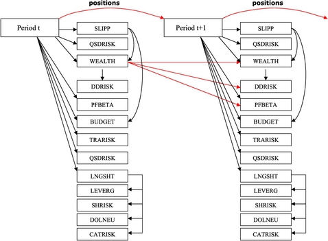
5.1 Key issues in model rollover
When the model in (43) is applied for portfolio rebalancing at some point in time, say ![]() , then the investor must first choose a suitable number of trading model periods T as well as respective period lengths (say, a day) for each of the T periods. Then, the model is initiated with root node at time
, then the investor must first choose a suitable number of trading model periods T as well as respective period lengths (say, a day) for each of the T periods. Then, the model is initiated with root node at time ![]() . For ease of exposition, suppose the money manager is interested in (actual) rebalancing of the portfolio at pre-specified time epochs
. For ease of exposition, suppose the money manager is interested in (actual) rebalancing of the portfolio at pre-specified time epochs ![]() (
(![]() ). To assure optimized rebalancing at each of these time epochs, the model in (43) is applied at each time
). To assure optimized rebalancing at each of these time epochs, the model in (43) is applied at each time ![]() ,
, ![]() , with its own multistage scenario tree. We will assume that each of these trees will have T periods, see Figure 4. Let the sequence of optimized rebalanced positions determined for each trading time
, with its own multistage scenario tree. We will assume that each of these trees will have T periods, see Figure 4. Let the sequence of optimized rebalanced positions determined for each trading time ![]() , using the model in (43), is herein denoted by
, using the model in (43), is herein denoted by ![]() ,
, ![]() , which are established in the market for the length of time
, which are established in the market for the length of time ![]() , referred to as the ith trading segment. Thus, it is only appropriate that the model in (43), applied at trading time
, referred to as the ith trading segment. Thus, it is only appropriate that the model in (43), applied at trading time ![]() , has specified a first period of length
, has specified a first period of length ![]() . Period lengths are indirectly incorporated into the model via the required forecasted parameters such as the mean vector
. Period lengths are indirectly incorporated into the model via the required forecasted parameters such as the mean vector ![]() , variance–covariance matrix
, variance–covariance matrix ![]() , security beta vector
, security beta vector ![]() , and the market index parameters
, and the market index parameters ![]() and
and ![]() . In addition, a scenario generator is required that is adapted to the period lengths in the model.
. In addition, a scenario generator is required that is adapted to the period lengths in the model.

There are several pertinent issues that must be addressed in a successful implementation. The treatment here is cursory, as the focus in this chapter is model development and its performance analyses. First, while the first period length is set to ![]() (at trading time
(at trading time ![]() ), the remaining period lengths (of the
), the remaining period lengths (of the ![]() periods) need not necessarily correspond to the actual trading epochs. One reason for this is that the computational solution of the model (43) is realistic only for a modest number of periods, for instance, T being not more than 3 or 4. But in order to capture the price dynamics in the future, periods of increasing length may be specified. For infinite horizon problems modeled as finite stage models, Grinold (1986) describes constructing an end effects period to capture the dynamics of the future after a finite number of model periods. For instance, see Cariño, Myers and Ziemba (1998) for an application in financial planning that incorporate end effects periods. In the implementation and the computational results reported in the next section, we pick the period lengths quite arbitrarily, and these lengths remain fixed at all subsequent model rollovers.
periods) need not necessarily correspond to the actual trading epochs. One reason for this is that the computational solution of the model (43) is realistic only for a modest number of periods, for instance, T being not more than 3 or 4. But in order to capture the price dynamics in the future, periods of increasing length may be specified. For infinite horizon problems modeled as finite stage models, Grinold (1986) describes constructing an end effects period to capture the dynamics of the future after a finite number of model periods. For instance, see Cariño, Myers and Ziemba (1998) for an application in financial planning that incorporate end effects periods. In the implementation and the computational results reported in the next section, we pick the period lengths quite arbitrarily, and these lengths remain fixed at all subsequent model rollovers.
The second important issue is the estimation of parameters (of random vectors) for the chosen periods, conditional upon the observed history of actual price series. Suppose the actual price (vector) is denoted by ![]() at time τ. Thus, when forecasting the parameters for trading segment 1 at time
at time τ. Thus, when forecasting the parameters for trading segment 1 at time ![]() , one must use historical prices (only) from the realized history
, one must use historical prices (only) from the realized history ![]() , which will be applied at node
, which will be applied at node ![]() of the model. Thereafter, for all forecasts at an arbitrary node
of the model. Thereafter, for all forecasts at an arbitrary node ![]() of the model, only the actual observations
of the model, only the actual observations ![]() must be used; however, they may be adapted to the particular (generated) scenario
must be used; however, they may be adapted to the particular (generated) scenario ![]() being followed in the scenario tree.
being followed in the scenario tree.
For the implementation in Section 6, second moment forecasts (variances and correlations) remain fixed at all nodes ![]() and set equal to those at the root node
and set equal to those at the root node ![]() . However, the first moment forecasts computed at the root node
. However, the first moment forecasts computed at the root node ![]() are progressively adapted to the scenario outcomes being followed up to a given node
are progressively adapted to the scenario outcomes being followed up to a given node ![]() . This adaptation procedure or the computation of the root node forecasts themselves are highly specialized and are omitted from further discussion in this chapter. The subject of parameter estimation in the context of financial market data has received considerable attention and there is a wealth of literature on various methods. The interested reader is referred to, for instance, Andreou and Ghysels (2002), Bai, Russell and Tiao (2001), Cohen et al. (1983), Foster and Nelson (1996), Ledoit and Wolf (2003), Merton (1980), and Scholes and Williams (1977).
. This adaptation procedure or the computation of the root node forecasts themselves are highly specialized and are omitted from further discussion in this chapter. The subject of parameter estimation in the context of financial market data has received considerable attention and there is a wealth of literature on various methods. The interested reader is referred to, for instance, Andreou and Ghysels (2002), Bai, Russell and Tiao (2001), Cohen et al. (1983), Foster and Nelson (1996), Ledoit and Wolf (2003), Merton (1980), and Scholes and Williams (1977).
Between two model rollovers, say from ![]() to
to ![]() , the optimized portfolio must be evaluated based on the actual price series, herein termed portfolio (out-of-sample) simulation and it represents the actual performance of the portfolio under model-specified trade-sizes. Therefore, the actual (initial) portfolio wealth for a model-run beginning at the trading epoch at
, the optimized portfolio must be evaluated based on the actual price series, herein termed portfolio (out-of-sample) simulation and it represents the actual performance of the portfolio under model-specified trade-sizes. Therefore, the actual (initial) portfolio wealth for a model-run beginning at the trading epoch at ![]() , denoted by
, denoted by ![]() , is given by
, is given by ![]() , where
, where ![]() is the discount rate adjusted to the trading segment length
is the discount rate adjusted to the trading segment length ![]() .
. ![]() is the wealth at the inception of the portfolio at the beginning of the first trading epoch
is the wealth at the inception of the portfolio at the beginning of the first trading epoch ![]() . Then, the portfolio value series, under the model-based continuous rollover rebalancing, is the wealth sequence
. Then, the portfolio value series, under the model-based continuous rollover rebalancing, is the wealth sequence ![]() , which is evaluated for performance.
, which is evaluated for performance.
5.2 Portfolio performance metrics
The rebalancing model in (43) is evaluated by computing performance metrics for the (simulated) wealth series ![]() of the managed portfolio. These performance metrics are
of the managed portfolio. These performance metrics are
The last two drawdown metrics have not been considered in the literature, to the best of the author’s knowledge. However, they provide key metrics of performance evaluation that are critical for successful money management.
6 Model application
SPDR Trust, which is an exchange-traded fund that holds all of the S&P 500 index stocks, is used as the market barometer in portfolio rebalancing. SPDR trades under the ticker symbol SPY. The model is applied for managing a portfolio of 95 stocks chosen from the Standard and Poors 100 stocks. These stocks are listed in Table 1. The full data set for the experimentation covers the period from January 02, 1996 to August 16, 2002. A period of 200 days of history, immediately preceding the beginning day (i.e., root node) of the multiperiod decision model, is used to estimate required parameters for the RoR random vectors. That is, the first trading segment begins on day 202, ![]() , on October 16, 1996. Thus, when applying the model for the trading segment
, on October 16, 1996. Thus, when applying the model for the trading segment ![]() , the historical data period used is from day
, the historical data period used is from day ![]() to day
to day ![]() . The model is used for actual daily rebalancing of the portfolio, which thus results in 1450 rollovers of the model. That is, trade segment lengths are each a day long,
. The model is used for actual daily rebalancing of the portfolio, which thus results in 1450 rollovers of the model. That is, trade segment lengths are each a day long, ![]() , for
, for ![]() . The model is run in three versions,
. The model is run in three versions, ![]() , and 3. The model period lengths are first period length = 1 day, second period length = 4 days, and the third period length = 5 days. So, in a 3-stage model (i.e.,
, and 3. The model period lengths are first period length = 1 day, second period length = 4 days, and the third period length = 5 days. So, in a 3-stage model (i.e., ![]() ), the total time horizon is 10 days into the future.
), the total time horizon is 10 days into the future.

Techniques for generating scenarios for multistage stochastic programs have been investigated at great length, however, there is no one procedure that is best suited for varied applications. The reader interested in scenario generation methods for financial planning problems is referred to, for instance, Gulpinar, Rustem and Settergren (2004), Høyland and Wallace (2001), Kouwenberg (2001), Mulvey (1996), Mulvey, Morin and Pauling (1999), Mulvey, Rosenbaum and Shetty (1999), Pflug (2000), Yu, Ji and Wang (2003) and the many references therein. The generation method implemented with our rebalancing system is based on using the Mahalanobis distance-metric, applied on the historical return series and calibrated to market conditions, see Edirisinghe and Patterson (2003). Each scenario outcome at a given node ![]() is 95-dimensional. To generate a small enough sample that achieves the intended risk management properties, the scenario generation schemes utilized are highly specialized. The details of these schemes are outside the scope of this chapter.
is 95-dimensional. To generate a small enough sample that achieves the intended risk management properties, the scenario generation schemes utilized are highly specialized. The details of these schemes are outside the scope of this chapter.
For the experimentation period indicated above, the SPY index performance is used as a surrogate for the market performance, and its performance metrics are presented in Table 2, also see Figure 5 for its daily performance. Cash positions are applied an annualized money market rate of ![]() , which thus serves as the riskfree rate. All experiments begin with an initial wealth of $1 million available on
, which thus serves as the riskfree rate. All experiments begin with an initial wealth of $1 million available on ![]() 202, and no further exogenous cash flow is available at any time. The initial positions in all risky securities at the beginning of segment
202, and no further exogenous cash flow is available at any time. The initial positions in all risky securities at the beginning of segment ![]() (on October 15, 1996) are set to zero. All model runs allow both long and short trades with no shortsale constraints. Transactions cost (TC) parameters, see (4), are
(on October 15, 1996) are set to zero. All model runs allow both long and short trades with no shortsale constraints. Transactions cost (TC) parameters, see (4), are ![]() and
and ![]() for all stocks. The effects of increased cost rates will be illustrated later.
for all stocks. The effects of increased cost rates will be illustrated later.
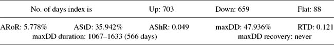
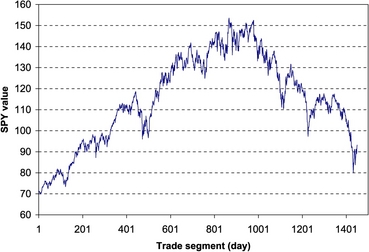
6.1 Single stage models
The first set of experiments is concerned with analysing the one period model version with varied risk metrics to highlight the relative effects of risk controls. With only SRC applied on one period models, scenarios of uncertainty are not required. These experiments compare SRC risk metrics: TRARISK ![]() in (24), CATRISK
in (24), CATRISK ![]() in (26), and the (variance) risk metric
in (26), and the (variance) risk metric ![]() , MARKOW. Pure SRC control means only one SRC metric is applied at a time. Table 3 provides a representative summary of portfolio performance for this case, where each column corresponds to a particular value of the objective risk aversion coefficient. See Figures 6 and 7 for a comparison of main portfolio performance measures across pure SRC metrics.
, MARKOW. Pure SRC control means only one SRC metric is applied at a time. Table 3 provides a representative summary of portfolio performance for this case, where each column corresponds to a particular value of the objective risk aversion coefficient. See Figures 6 and 7 for a comparison of main portfolio performance measures across pure SRC metrics.

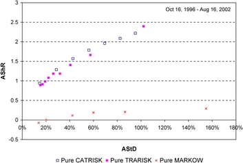

Pure (Markowitz) variance risk metric performs extremely poorly at all attempted coefficients of risk aversion, and none of the performance metrics appear to be within acceptable ranges for fund management. The strategy that achieves a Reward-to-Drawdown ratio of at least 2 with the least maxDD (of 16.86%) is the Pure CatRisk strategy. Even this level of drawdown may be unacceptable to a fund manager, even though it has ARTD > 2. By following a mixed strategy in which two SRC metrics are applied simultaneously, one may obtain improved portfolio performance. This is demonstrated next using tracking control and Cat risk control together. Tracking risk aversion coefficient is applied at five different levels: Very Low, Low, Moderate, High, and Very High. For each of these levels, Cat risk is varied to plot portfolio performance, as given in Figures 8 and 9. In each of these two plots, the upper envelope may be thought of as the appropriate frontier in the two-dimensional risk metric space. Furthermore, Drawdown Duration to Drawdown Recovery time ratio, or DDDR ratio, for the mixed strategy (with moderate tracking aversion coefficient) remained between 0.33 and 0.55. A DDDR ratio of greater than 1 is desirable. DDDR for the pure (Markowitz) variance risk metric was zero because the portfolio never recovered from its maximum drawdown, for all ranges of variance risk aversion coefficients, during the invested period.
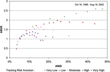
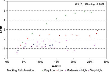
Under two-dimensional integrated SRC, the rebalancing strategy that achieves ARTD just over 2.0, with the lowest maxDD%, corresponds to a run of “Low” tracking risk aversion with CatRisk of $10,000 a day. This run has Return-to-Drawdown ARTD = 2.04 with maxDD = 6.07%, AShR = 1.44, and ARoR = 16.40%. The portfolio value over time for this run is depicted in Figure 10. In the same figure, two other graphs are plotted: the run that corresponds to the maximum ARTD of 4.89 (with a maxDD of 23.32%, AshR = 2.59, and ARoR = 118.14% for the pair “Very Low” tracking risk aversion and daily CatRisk = $60,000) and the run under “moderate” tracking risk aversion and daily CatRisk = $50,000 which yields the highest Sharpe ratio (AShR = 1.63, with maxDD = 14.53%, ARTD = 1.79 and ARoR = 30.01%). For these three cases, portfolio daily standard deviations are in Figure 11 and the daily portfolio betas are in Figure 12.
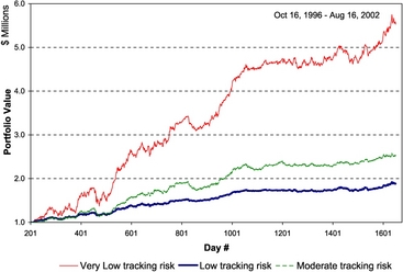
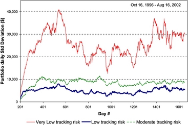

6.2 Comparison with multistage models
Two-stage models are specified with a day-long first stage and a second stage of 4 days, for a future horizon of 5 days. Three stage models have a third stage of 5 days, for a 10 day-horizon. Multistage models, generally, are better able to trade-off transaction costs and control drawdown. Multistage models too are rolled over the 1450 trading days. Given that both Cat risk and Tracking risk in combination provided better risk control in single stage models, the multistage runs have this dual risk control settings. Portfolio variance as a risk metric (i.e., Markowitz metric) performs poorly even in the case of 2-stage models. To illustrate, the 2-stage model is run with pure variance (MARKOW) risk metric, and it is compared with a non-MARKOW model with SRC/DRC metrics, but with the same value for objective (quadratic) risk aversion coefficients. The non-MARKOW model had CatRisk = $40,000 and drawdown risk metric with ![]() . Portfolio trajectories and portfolio standard deviations are shown in Figures 13 and 14, respectively.
. Portfolio trajectories and portfolio standard deviations are shown in Figures 13 and 14, respectively.


A comparison of risk-return trade-off between 1- and 2-stage models is presented next, where the effects of transactions/market impact costs are also pursued. The per-share cost rate ![]() , set at 2% in the experiments so far, is increased to 5%. The two model versions have the exact same settings, except for the number of model periods, where the 2-period model is specified with
, set at 2% in the experiments so far, is increased to 5%. The two model versions have the exact same settings, except for the number of model periods, where the 2-period model is specified with ![]() (95-dimensional) return scenarios for the 5 day period. This analysis reveals two important properties in rebalancing. First, at a fixed transactions cost rate, 2-stage models perform better than 1-stage models. Second, as the transactions costs increase, the advantages of multistage models over single period models become increasingly prominent. These effects are captured in Figures 15-18. As the last figure indicates, 2-stage model performance is quite robust in the event trading costs increase.
(95-dimensional) return scenarios for the 5 day period. This analysis reveals two important properties in rebalancing. First, at a fixed transactions cost rate, 2-stage models perform better than 1-stage models. Second, as the transactions costs increase, the advantages of multistage models over single period models become increasingly prominent. These effects are captured in Figures 15-18. As the last figure indicates, 2-stage model performance is quite robust in the event trading costs increase.
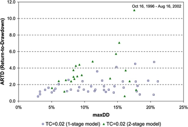
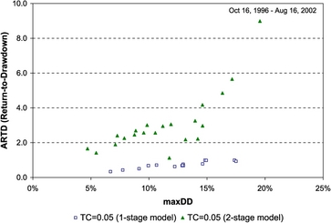


Portfolio rebalancing using models with 3 periods yields significantly better performance with regard to drawdown characteristics. This is due to applying the drawdown risk (DDR) control, see (40), over 3 period-scenarios of the model. The drawdown duration to recovery ratios (DDDR) are compared across 1-, 2-, and 3-stage models with allowable relative drawdown set at 10% and specifying a very high drawdown risk aversion coefficient. These runs correspond to a “moderate” tracking risk aversion, for various levels of CatRisk control. As can be seen from Figure 19, these multistage models have rather impressive improvements over the single period counterpart.

7 Concluding remarks
This article discussed an integrated risk management paradigm for frequent rebalancing of a portfolio of securities, using multistage stochastic programming modeling. By mathematically representing many practically useful risk metrics for fund management, the model is able to provide very effective rebalancing strategies. In particular, with impressive improvements in portfolio drawdown characteristics, such a stochastic programming based model can become an invaluable tool for money managers.
There are various other related issues that have escaped discussion in this article—for instance, market parameter estimations, methods for scenario projections to describe future uncertainty, as well as various other practical issues faced by money managers. In particular, trade execution costs are treated within simple slippage models in this paper, but the actual costs can be quite substantial and modeling those costs can be quite complicated. Also, the stochastic programming model considered here specifies trades as continuous variables, while in practice, trades must be integral, and they are typically lot-sized for execution. The latter requirement would lead to integer stochastic programming models and the solution of such models is generally tedious for real-time implementations of portfolio problems of practical size.
Finally, it was assumed that the universe of securities is pre-specified for the model to determine optimal trades. In a more successful implementation, such a universe must be determined and modified at regular intervals of time, based on considerations other than portfolio risk management. There are no standard techniques for such security selections, although practitioners use either fundamental analysis (of individual issues or market sectors/industries), tools from technical analysis (see, for example, Achelis (2000)), or a combination of both. Edirisinghe and Zhang (2004) describe a procedure based on fundamental analysis (of company income and balance sheets) in which optimization techniques are applied for identifying candidates for the universe of securities for portfolio risk management.
Acknowledgement
The assistance received from Maksym Bychkov and Ike Patterson in implementing the trade rebalancing system is thankfully acknowledged. Also, thanks are due to the SRGP program, College of Business, University of Tennessee, for the financial support received during the initial stages of the research in 2001.
References
S.B. Achelis. Technical Analysis from A to Z, second ed. McGraw-Hill; 2000.
E. Andreou, E. Ghysels. Rolling-sample volatility estimators: some new theoretical, simulation and empirical results. Journal of Business and Economic Statistics. 2002;20:363-376.
P. Artzner, F. Delbaen, J.-M. Eber, D. Heath. Coherent measures of risk. Mathematical Finance. 1999;9:203-228.
Bai, X., Russell, J.R., Tiao, G.C., 2001. Beyond Merton’s utopia (I): Effects of non-normality and dependence on the precision of variance estimates using high-frequency financial data, Working Paper. University of Chicago
J.R. Birge, N.C.P. Edirisinghe, W.T. Ziemba, editors. Research in Stochastic Programming. Annals of Operations Research, vol. 100. 2001. Baltzer Science Publishers.
J.R. Birge, F. Louveaux. Introduction to Stochastic Programming. New York: Springer-Verlag; 1997.
S.P. Bradley, D.B. Crane. A dynamic model for bond portfolio management. Management Science. 1972;19:139-151.
Bychkov, M., Edirisinghe, N.C.P., 2004. Approximating scenarios for financial investment models using CVaR information, Working Paper. College of Business, University of Tennessee
D.R. Cariño, D. Myers, W.T. Ziemba. Concepts, technical issues and uses of the Russell–Yasuda-Kasai financial planning model. Operations Research. 1998;46(4):450-462.
D.R. Cariño, W.T. Ziemba. Formulation of the Russell–Yasuda-Kasai financial planning model. Operations Research. 1998;46(4):433-449.
D.R. Cariño, T. Kent, D.H. Myers, C. Stacy, M. Sylvanus, A.L. Turner, K. Watanabe, W.T. Ziemba. The Russell–Yasuda Kasai model: An asset/liability model for a Japanese insurance company using multistage stochastic programming. Interfaces. 1994;24(1):29-49.
S. Chekhlov, S. Uryasev, M. Zabarankin. Portfolio optimization with drawdown constraints. In: B. Scherer, editor. Asset and Liability Management Tools. London: Risk Books; 2003:263-278.
K.J. Cohen, G.A. Hawawini, S.F. Maier, R.A. Schwartz, D.K. Whitcomb. Estimating and adjusting for the intervalling-effect bias in beta. Management Science. 1983;29:135-148.
G. Consigli, M.A.H. Dempster. The CALM stochastic programming model for dynamic asset and liability management. In: W.T. Ziemba, J.M. Mulvey, editors. Worldwide Asset and Liability Modeling. Cambridge University Press; 1998:464-500.
A. Consiglio, F. Cocco, S.A. Zenios. The value of integrative risk management for insurance products with guarantees. Journal of Risk Finance. 2001:1-11.
J. Cvitanic, I. Karatzas. On portfolio optimization under drawdown constraints. IMA Lecture Notes in Mathematics and Applications. 1995;65:77-88.
Delbaen, F., 2000. Coherent risk measures on general probability spaces, Working Paper. ETH, Zurich
R.S. Dembo, A.J. King. Tracking models and the optimal regret distribution in asset allocation. Applied Stochastic Models and Data Analysis. 1992;8:151-157.
Dert, C., 1995. Asset liability management for pension funds, PhD thesis. Erasmus University, Rotterdam, Netherlands
N.C.P. Edirisinghe. Bound-based approximations in multistage stochastic programming: nonanticipativity aggregation. Annals of Operations Research. 1999;85:103-127.
Edirisinghe, N.C.P., 2004. Multiperiod portfolio optimization with terminal liability: Bounds for the convex case, Computational Optimization and Applications
N.C.P. Edirisinghe, V. Naik, R. Uppal. Optimal replication of options with transactions costs and trading restrictions. Journal of Financial and Quantitative Analysis. 1993;28:117-138.
Edirisinghe, N.C.P., Patterson, E.I., 2003. Scenario generation for financial stochastic programs using Mahalanobis distance metric, Presentation at INFORMS, Atlanta, Oct. 2003 and Working Paper. College of Business, Univ. of Tennessee
Edirisinghe, N.C.P., Patterson, E.I., 2007. Multiperiod stochastic portfolio optimization: Block-separable decomposition. Annals of Operations Research, in press
Edirisinghe, N.C.P., Zhang, X., 2004. Stock selection for portfolio optimization via data envelopment analysis of financial statements: Empirical evidence, Working Paper. College of Business, Univ. of Tennessee
N.C.P. Edirisinghe, W.T. Ziemba. Tight bounds for stochastic convex programs. Operations Research. 1992;40(4):660-677.
N. El-Hassan, P. Kofman. Tracking error and active portfolio management. Australian Journal of Management. 2003;28(2):183-208.
H. Follmer, A. Schied. Convex measures of risk and trading constraints. Finance and Stochastics. 2002;6:429-447.
D.P. Foster, D.B. Nelson. Continuous record asymptotics for rolling sample variance estimators. Econometrica. 1996;64:139-174.
K. Frauendorfer. Barycentric scenario trees in convex multistage stochastic programming. Mathematical Programming. 1996;75(2):277-294.
A. Frino, D.R. Gallagher. Tracking S&P 500 Index funds. Journal of Portfolio Management. 2001;28:44-55.
Geyer, A., Herold, W., Kontriner, K., Ziemba, W.T., 2003. The Innovest Austrian Pension Fund financial planning model InnoALM, Working Paper. Sauder School of Business, University of British Columbia
B. Golub, M. Holmer, R. McKendall, L. Pohlman, S.A. Zenios. Stochastic programming models for money management. European Journal of Operational Research. 1997;85:282-296.
R.C. Grinold. Infinite horizon stochastic programs. SIAM Journal of Control and Optimization. 1986;24:1246-1260.
S.J. Grossman, Z. Zhou. Optimal Investment strategies for controlling drawdowns. Mathematical Finance. 1993;3(3):241-276.
N. Gulpinar, B. Rustem, R. Settergren. Multistage stochastic mean-variance portfolio analysis with transaction costs. In: A. Nagurney, editor. Innovations in Financial and Economic Networks. Edward Elgar Publishing; 2003:46-66.
N. Gulpinar, B. Rustem, R. Settergren. Optimisation and simulation approaches to scenario tree generation. Journal of Economic Dynamics and Control. 2004;28:1291-1315.
M.R. Holmer, S.A. Zenios. The productivity of financial intermediation and the technology of financial product management. Operations Research. 1995;43(6):970-982.
Høyland, K., 1998. Asset liability management for a life insurance company: A stochastic programming approach, PhD thesis. Norwegian University of Science and Technology, Trondheim, Norway
K. Høyland, S.W. Wallace. Generating scenario trees for multi stage problem. Management Science. 2001;47(2):295-307.
B.I. Jacobs, K.N. Levy. Market Neutral Strategies. John Wiley and Sons Inc; 2004.
R. Jansen, R. van Dijk. Optimal benchmark tracking with small portfolios. Journal of Portfolio Management. 2002;29:33-49.
R. Jarrow. Put option premiums and coherent risk measures. Mathematical Finance. 2002;12:125-134.
D.B. Keim, A. Madhavan. The upstairs market for large-block transactions: analysis and measurement of price effects. Review of Financial Studies. 1996;9:1-36.
D.B. Keim, A. Madhavan. Transaction costs and investment style: an interexchange analysis of institutional equity trades. Journal of Financial Economics. 1997;46:265-292.
D.B. Keim, A. Madhavan. The cost of institutional equity trades. Financial Analysts Journal. 1998;54(4):50-69.
H. Konno, K. Kobayashi. An integrated stock-bond portfolio optimization model. Journal of Economic Dynamics and Control. 1997;21:1427-1444.
H. Konno, H. Yamazaki. Mean-absolute deviation portfolio optimization model and its applications to Tokyo stock market. Management Science. 1991;37(5):519-531.
R. Kouwenberg. Scenario generation and stochastic programming models for asset liability management. European Journal of Operational Research. 2001;134:279-292.
M.I. Kusy, W.T. Ziemba. A bank asset and liability management model. Operations Research. 1986;34(3):356-376.
O. Ledoit, M. Wolf. Improved estimation of the covariance matrix of stock returns with an application to portfolio selection. Journal of Empirical Finance. 2003;10(5):603-621.
T.F. Loeb. Trading cost: the critical link between investment information and results. Financial Analysts Journal. 1983;39:39-43.
H.M. Markowitz. Portfolio selection. Journal of Finance. 1952;7:77-91.
H.M. Markowitz. Portfolio Selection—Efficient Diversification of Investments. New York: John Wiley; 1959.
H.M. Markowitz. Mean-Variance Analysis in Portfolio Choice and Capital Markets. Oxford: Blackwell; 1987.
R.C. Merton. On estimating the expected return on the market: An exploratory investigation. Journal of Financial Economics. 1980;8:323-361.
J.M. Mulvey. Generating scenarios for the Towers Perrin investment system. Interfaces. 1996;26(2):1-15.
J.M. Mulvey, G. Gould, C. Morgan. An asset and liability management system for Towers Perrin–Tillinghast. Interfaces. 2000;30(1):96-114.
J.M. Mulvey, F. Morin, B. Pauling. Calibration of stochastic scenario generators for DFA. Annals of Operations Research. 1999;85:249-266.
J.M. Mulvey, D.P. Rosenbaum, B. Shetty. Parameter estimation in stochastic scenario generation systems. European Journal of Operations Research. 1999;118:563-577.
J. Mulvey, H. Vladimirou. Stochastic network programming for financial planning under uncertainty. Management Science. 1992;18:1642-1664.
J.G. Nicholas. Market-Neutral Investing: Long/Short Hedge Fund Strategies. Bloomberg Press; 2000.
S. Nielsen, S.A. Zenios. A stochastic model for funding single premium deferred annuities. Mathematical Programming. 1996;75:177-200.
W. Ogryczak, A. Ruszczynski. From stochastic dominance to mean-risk models: Semi-deviations as risk measures. European Journal of Operational Research. 1999;116:33-50.
W. Ogryczak, A. Ruszczynski. Dual stochastic dominance and related mean-risk models. SIAM Journal of Optimization. 2002;13(1):60-78.
G.C. Pflug. Scenario tree generation for multiperiod financial optimization by optimal discretization. Mathematical Programming. 2000;89:251-271.
R.T. Rockafellar, S. Uryasev. Optimization of conditional value-at-risk. The Journal of Risk. 2000;2(3):21-41.
Rockafellar, R.T., Uryasev, S., Zabarankin, M., 2002. Deviation measures in risk analysis and optimization, Research Report 2002-7. Department of Industrial and Systems Engineering, University of Florida
R. Roll. A mean-variance analysis of tracking error. Journal of Portfolio Management. 1992;18:13-22.
Roorda, B., Engwerda, J., Schumacher, H., 2002. Coherent acceptability measures in multiperiod models, Working Paper. University of Twente
M. Scholes, J. Williams. Estimating betas from nonsynchronous data. Journal of Financial Economics. 1977;5:309-327.
W.F. Sharpe. The Sharpe ratio. Journal of Portfolio Management. 1994:49-58.
M.C. Steinbach. Markowitz revisited: Mean-variance models in financial portfolio analysis. SIAM Review. 2001;43(1):31-85.
N.G. Torre, M.J. Ferrari. The market impact model. http://mim.barra.com/research/misc/market-impact-model.pdf. BARRA Research Insights
M.H. van der Vlerk. Stochastic programming bibliography. World Wide Web http://mally.eco.rug.nl/spbib.html.
J. von Neumann, O. Morgenstern. Theory of Games and Economic Behavior. Princeton University Press; 1944.
M. Warachka, Y. Zhao, W.T. Ziemba. Incorporating Diversification into Risk Management. Research Paper Series, 2004.
G.A. Whitmore, M.C. Findlay. Stochastic Dominance: An Approach to Decision Making under Risk. Lexington, MA: Heath; 1978.
L.Y. Yu, X.D. Ji, S.Y. Wang. Stochastic programming models in financial optimization: a survey. Advanced Modeling and Optimization. 2003;5(1):1-26.
S.A. Zenios. Financial Optimization. Cambridge, England: Cambridge University Press; 1993.
S.A. Zenios. Asset/liability management under uncertainty for fixed-income securities. Annals of Operations Research. 1995;59:77-98.
Y. Zhao, W.T. Ziemba. A stochastic programming model using an endogenously determined worst case risk measure for dynamic asset allocation. Mathematical Programming. 2001;89:293-309.
W.T. Ziemba. The Stochastic Programming Approach to Asset, Liability, and Wealth Management. AIMR/Blackwell Publisher; 2003.
W.T. Ziemba, J. Mulvey. World Wide Asset and Liability Modeling. Cambridge University Press; 1998.
W.T. Ziemba, R.G. Vickson, editors. Stochastic Optimization Models in Finance. Academic Press, 1975.