Chapter 9: Components That Group Data

In This Chapter

• Showing top and bottom views

• Tracking progress using histograms

• Emphasizing top values in charts

It’s often helpful to organize your data into logical groups. Grouping allows you to focus on manageable sets of information that have key attributes. For example, instead of looking at all customers in one giant view, you can analyze customers who buy only one product. This allows you to focus attention and resources on those customers who have the potential to buy more products. The benefit is that you can more easily pick out groups that fall outside the norm for your business.

In this chapter, you focus on how you can organize groups of data using dashboard components.

Listing Top and Bottom Values

When you look at the list of Fortune 500 companies, you often look for the top 20 companies. Then perhaps you look at who eked out at the bottom 20 slots. It’s unlikely that you check to see which company came in at number 251. It’s not necessarily because you don’t care about number 251; it’s just that you can’t spend the time or energy to process all 500 companies. So you process the top and bottom of the list.

This is the same concept behind creating top and bottom displays. Your audience has only a certain amount of time and resources to dedicate to solving any issues you can emphasize in your dashboard. Showing them the top and bottom values in your data can help them pinpoint where and how they can have the most impact with the time and resources they do have.

Organizing source data

The top and bottom displays you create can be as simple as source data that you incorporate into your dashboard. Typically placed to the right of a dashboard, this data can emphasize details a manager may use to take action on a metric. For example, the simple dashboard in Figure 9-1 shows sales information with top and bottom sales reps.

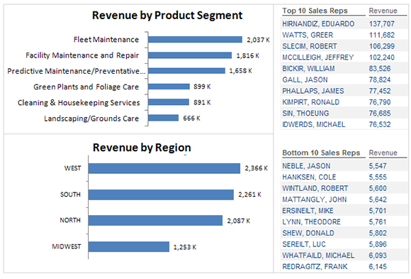
Figure 9-1: Top and bottom displays that emphasize certain metrics.

To get a little fancier, you can supplement your top and bottom displays with some ranking information, some in-cell bar charts, or some conditional formatting (see Figure 9-2).

You can create the in-cell bar charts with the Data Bars conditional formatting function, covered in Chapter 4. The arrows are also simple conditional formatting rules that are evaluated against the variance in current and last months’ ranks.

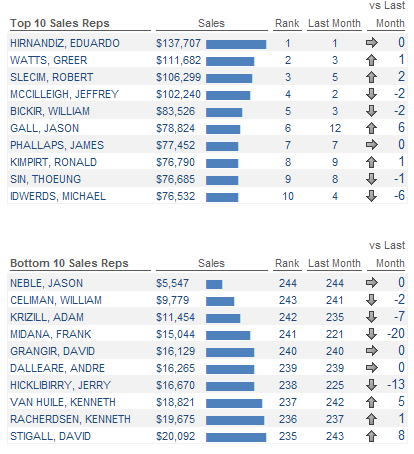
Figure 9-2: You can use some conditional formatting to add visual components to your top and bottom displays.

Using pivot tables to get top and bottom views

A pivot table is an amazing tool that can help you create interactive reporting. If you’re new to pivot tables, fear not. You learn about them in detail in Part IV of this book. For now, take a moment to go through an example of how pivot tables can help you build interactive top and bottom displays.

You can open the Chapter 9 Samples.xlsx file, found on this book’s companion website at www.wiley.com/go/exceldr to follow along.

Follow these steps to display a Top filter with a pivot table:

1. Start with a pivot table that shows the data you want to display with your top and bottom views.

In this case, the pivot table shows Sales Rep and Sales_Amount (see Figure 9-3).

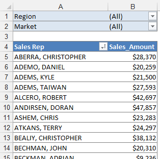
Figure 9-3: Start with a pivot table that contains the data you want to filter.

2. Right-click on the field you want to use to determine the top values. In this example, you use the Sales Rep field. Choose Filter→Top 10 (see Figure 9-4).

Figure 9-4: Select the Top 10 filter option.

The Top 10 Filter (Sales Rep) dialog box appears (see Figure 9-5).

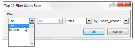
Figure 9-5: Specify the filter you want to apply.

3. In the Top 10 Filter (Sales Rep) dialog box, define the view you’re looking for. In this example, you want the Top 10 Items (Sales Reps) as defined by the Sales_Amount field.

4. Click OK to apply the filter.

At this point, your pivot table is filtered to show you the top ten sales reps for the selected Region and Market. You can change the Market filter to Charlotte and get the top ten sales reps for Charlotte only (see Figure 9-6).

5. To view the bottom ten Sales Rep list, copy the entire pivot table and paste it next to the existing one.

6. Repeat Steps 2–4 in the newly copied pivot table, except this time choose to filter on the bottom ten items as defined by the Sales_Amount field.

If all went well, you now have two pivot tables similar to Figure 9-7: one that shows the top ten sales reps and one that shows the bottom ten. You can link back to these two pivot tables in the analysis layer of your data model using formulas. This way, when you update the data, your top and bottom values display the new information.

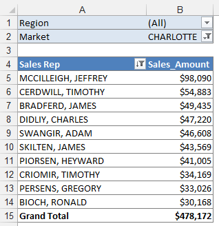
Figure 9-6: You can interactively filter your pivot table report to instantly show the top ten sales reps for any Region and Market.

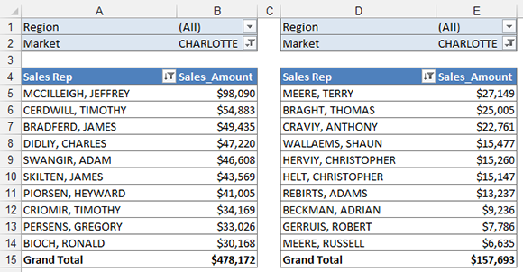
Figure 9-7: You now have two pivot tables that show top and bottom displays.

If there’s a tie for any rank in the top or bottom values, Excel shows you all the tied records. This means that you may get more than the number you filtered for. If you filtered for the top 10 sales reps and there’s a tie for the number 5 rank, Excel shows you 11 sales reps (both reps ranked at number 5 will be shown).

Using Histograms to Track Relationships and Frequency

A histogram is essentially a graph that plots frequency distribution. A frequency distribution shows how often an event or category of data occurs. With a histogram, you can visually see the general distribution of a certain attribute.

Take a look at the histogram shown in Figure 9-8. This histogram represents the distribution of units sold in one month among your sales reps. As you can see, most reps sell somewhere between 5 and 25 units per month. As a manager, you want the hump in the chart to move to the right — more people selling a higher number of units per month. So you set a goal to have a majority of your sales reps sell between 15 and 25 units within the next 3 months. With this histogram, you can visually track the progress toward that goal.

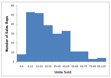
Figure 9-8: A histogram showing the distribution of units sold per month among your sales force.

This chapter discusses how to create a histogram using formulas and pivot tables. The techniques covered here fit nicely in data models where you separate data, analysis, and presentation information. In addition, these techniques allow for a level of automation and interactivity that comes in handy when updating dashboards each month.

We discuss how to develop a data model in Chapter 11.

Adding formulas to group data

First, you need a table that contains your raw data. The raw data ideally consists of records that represent unique counts for the data you want to group. For instance, the raw data table in Figure 9-9 contains unique sales reps and the number of units each has sold. Follow these steps to create a formula-driven histogram:

1. Before you create your histogram, you need to create a bin table (see Figure 9-9).

The bin table dictates the grouping parameters that are used to break your raw data into the frequency groups. The bin table tells Excel to cluster all sales reps selling fewer than 5 units into the first frequency group, any sales reps selling 5 to 14 units in the second frequency group, and so on.

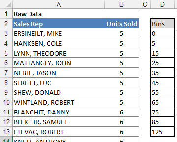
Figure 9-9: Start with your raw data table and a bin table.

You can freely set your own grouping parameters when you build your bin table. However, it’s generally a good idea to keep your parameters as equally spaced as possible. We typically end our bin tables with the largest number in our dataset. This allows us to have clean groupings that end in a finite number — not in an open-ended greater than designation.

2. Create a new column that holds the FREQUENCY formulas. Name the new column Frequency Formulas, as seen in Figure 9-10.

Excel’s FREQUENCY function counts how often values occur within the ranges you specify in a bin table.

3. Select a number of cells equal to the cells in your bin table.

4. Type the FREQUENCY formula you see in Figure 9-10 and then press Ctrl+Shift+Enter on your keyboard.

The FREQUENCY function does have a quirk that often confuses first-time users. The FREQUENCY function is an array formula — that is, it’s a formula that returns many values at one time. In order for this formula to work properly, you have to press Ctrl+Shift+Enter after typing the formula. If you just press the Enter key, you won’t get the results you need.

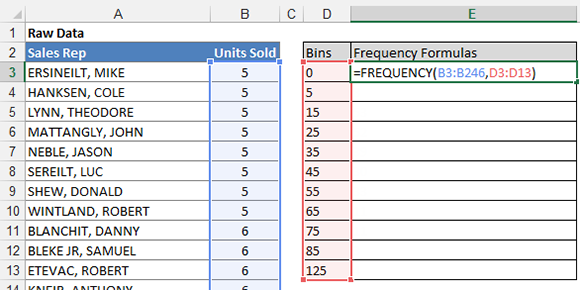
Figure 9-10: Type the FREQUENCY formula you see here; be sure to hold down the Ctrl+Shift+Enter keys on your keyboard.

At this point, you should have a table that shows the number of sales reps that fall into each of your bins. You could chart this table, but the data labels would come out wonky. For the best results, build a simple chart feeder table that creates appropriate labels for each bin, which you do as follows:

1. Create a new table that feeds the charts a bit more cleanly (see Figure 9-11). Use a simple formula that concatenates Bins into appropriate labels. Use another formula to bring in the results of your FREQUENCY calculations.

In Figure 9-11, we made the formulas in the first record of the chart feeder table visible. These formulas are essentially copied down to create a table appropriate for charting.

2. Use your newly created chart feeder table to plot the data into a column chart.

Figure 9-12 illustrates the resulting chart. You can certainly use the initial column chart as your histogram.

If you like your histograms to have spaces between the data points, you’re done. If you like the continuous blocked look you get with no gaps between the data points, follow the next few steps.

3. Right-click any of the columns in the chart and choose Format Data Series.

The Format Data Series dialog box appears.

4. Adjust the Gap Width property to 0% (see Figure 9-13).

Figure 9-11: Build a simple chart feeder table that creates appropriate labels for each bin.

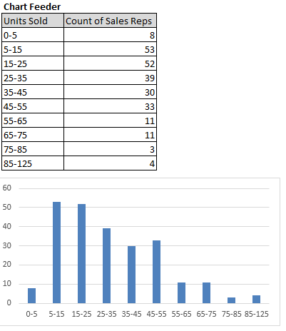
Figure 9-12: Plot your histogram data into a column chart.

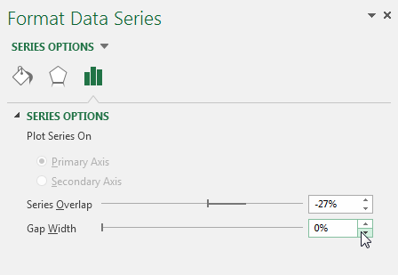
Figure 9-13: To eliminate the spaces between columns, set the Gap Width to 0%.

Adding a cumulative percent

A nice feature to add to your histograms is a cumulative percent series. With a cumulative percent series, you can show the percent distribution of the data points to the left of the point of interest.

Figure 9-14 shows an example of a cumulative percent series. At each data point in the histogram, the cumulative percent series tells you the percent of the population that fills all the bins up to that point. For instance, you can see that 25% of the sales reps denoted sold 15 units or fewer. In other words, 75% of the sales reps sold more than 15 units.

Take another look at the chart in Figure 9-14 and find the point where you see 75% on the cumulative series. At 75%, look at the label for that Bin range (you see 35–45). The 75% mark tells you that 75% of sales reps sold between 0 and 45 units. This means that only 25% of sales reps sold more than 45 units.

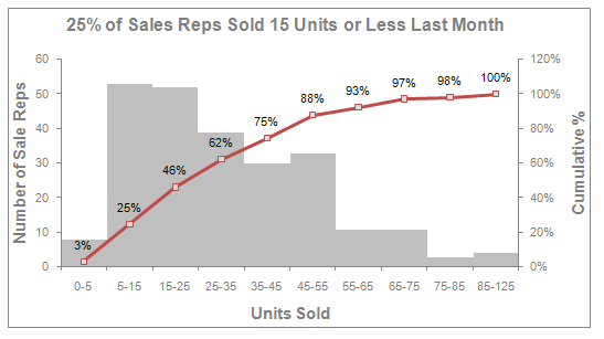
Figure 9-14: The cumulative percent series shows the percent of the population that fills all the bins up to each point in the histogram.

To create a cumulative percent series for your histogram, follow these steps:

1. After you perform Steps 1 through 5 to create a histogram (outlined earlier in this chapter), add a column to your chart feeder that calculates the percent of total sales reps for the first bin (see Figure 9-15).

Note the dollar symbols ($) used in the formula to lock the references while you copy the formula down.

Figure 9-15: In a new column, create a formula that calculates the percent of total sales reps for the first bin.

2. Copy the formula down for all the bins in the table.

3. Use the chart feeder table to plot the data into a line chart.

As you can see in Figure 9-16, the resulting chart needs some additional formatting.

Figure 9-16: Your initial chart will need some formatting to make it look like a histogram.

4. Right-click the series that makes up your histogram (Count of Sales Rep), select Change Chart Type, and then change the chart type to a column chart.

5. Right-click any of the columns in the chart and choose Format Data Series.

6. Adjust the Gap Width property to 0% (refer to Figure 9-13).

7. Right-click Cumulative Percent series and choose Format Data Series.

8. In the Format Data Series dialog box, change the Plot Series On option to Secondary Axis.

9. Right-click Cumulative Percent series and choose Add Data Labels.

At this point, your base chart is complete. It should look similar to the one shown at the beginning of this section in Figure 9-14. When you get to this point, you can adjust the colors, labels, and other formatting.

Using a pivot table to create a histogram

Did you know you can use a pivot table as the source for a histogram? That’s right. With a little-known trick, you can create a histogram that is as interactive as a pivot chart!

As in the formula-driven histogram, the first step in creating a histogram with a pivot table is to create a frequency distribution.

If you’re new to pivot tables, rest easy. In Part IV of this book, we cover the ins and outs of pivot tables. This section allows you to get a preview of the types of advanced analysis you can accomplish with pivot tables.

1. Create a pivot table and plot the data values in the row area (not the data area). As you can see in Figure 9-17, the SumOfSales Amount field is placed in the ROWS area. Place the Sales Rep field in the VALUES area as a Count.

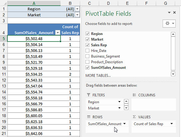
Figure 9-17: Place your data values in the ROWS area and the Sales Rep field in the VALUES area as a Count.

2. Right-click any value in the ROWS area and choose Group.

The Grouping dialog box appears (see Figure 9-18).

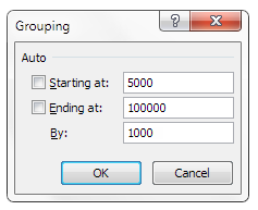
Figure 9-18: The Grouping dialog box.

3. In the dialog box, set the start and end values and then set the intervals.

This essentially creates your frequency distribution. In Figure 9-18, the distribution is set to start at 5,000 and to create groups in increments of 1,000 until it ends at 100,000.

4. Click OK to confirm your settings.

The pivot table calculates the number of sales reps for each defined increment, just as in a frequency distribution. (See Figure 9-19.) You can now leverage this result to create a histogram!

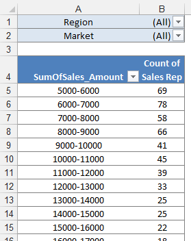
Figure 9-19: The result of grouping the values in the Row area is a frequency distribution that can be charted into a histogram.

The obvious benefit to this technique is that after you have a frequency distribution and a histogram, you can interactively filter the data based on other dimensions, like Region and Market. For instance, you can see the histogram for the Canada market and then quickly switch to see the histogram for the California market.

Note that you can’t add cumulative percentages to a histogram based on a pivot table.

Emphasizing Top Values in Charts

Sometimes a chart is indeed the best way to display a set of data, but you still want to call attention to the top values in that chart. In these cases, you can use a technique that actually highlights the top values in your charts. That is to say, you can use Excel to figure out which values in your data series are in the top nth value and then apply special formatting to them. Figure 9-20 illustrates an example where the top five quarters are highlighted and given a label.

The secret to this technique lies in Excel’s obscure LARGE function. The LARGE function returns the nth largest number from a dataset. In other words, you tell it where to look and the number rank you want.

To find the largest number in the dataset, you enter the formula LARGE(Data_Range, 1). To find the fifth largest number in the dataset, you use LARGE(Data_Range, 5). Figure 9-21 illustrates how the LARGE function works.

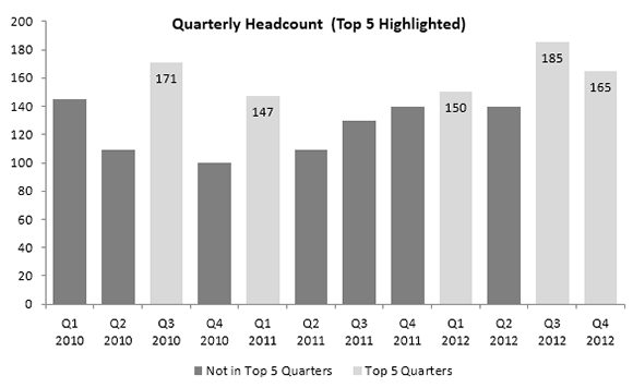
Figure 9-20: This chart highlights the top five quarters with different font and labeling.

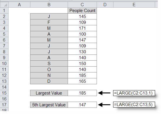
Figure 9-21: Using the LARGE function returns the nth largest number from a dataset.

The idea is fairly simple. In order to identify the top five values in a dataset, you first need to identify the fifth largest number (LARGE function to the rescue) and then test each value in the dataset to see if it’s bigger than the fifth largest number. Here’s what you do:

1. Build a chart feeder that consists of formulas that link back to your raw data. The feeder should have two columns: one to hold data that isn’t in the top five and one to hold data that is in the top five (see Figure 9-22).

2. In the first row of the chart feeder, enter the formulas shown in Figure 9-22.

The formula for the first column (F4) checks to see if the value in cell C4 is less than the number returned by the LARGE formula (the fifth largest value). If it is, the value in cell C4 is returned. Otherwise, NA is used. The formula for the second column works in the same way, except the IF statement is reversed: If the value in cell C4 is greater than or equal to the number returned by the LARGE formula, then the value is returned; otherwise NA is used.

3. Copy the formulas down to fill the table.

4. Use the chart feeder table to plot the data into a stacked column chart.

You immediately see a chart that displays two data series: one for data points not in the top five and one for data points in the top five (see Figure 9-23).

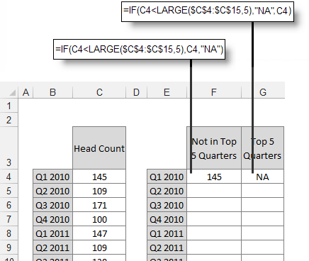
Figure 9-22: Build a new chart feeder that consists of formulas that plot values into one of two columns.

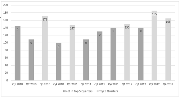
Figure 9-23: After adding data labels to the top five data series and doing a bit of formatting, your chart should look similar to the one shown here.

Notice in Figure 9-23 that the chart shows some rogue zeros. You can fix the chart so that the zeros don’t display by performing the next few steps.

5. Right-click any of the data labels for the top five series and choose Format Data Labels.

6. In the Format Data Labels dialog box, expand the Numbers section and select Custom in the Category list.

7. Enter #,##0;; as the custom number format, as shown in Figure 9-24.

8. Click the Add button and then click Close.

Figure 9-24: Entering #,##0;; as the custom format for a data label renders all zeros in that data series hidden.

When you go back to your chart, you see that the rogue zeros are now hidden and your chart is ready for colors, labels, and other formatting you want to apply.

You can apply the same technique to highlight the bottom five values in your data set. The only difference is that instead of using the LARGE function, you use the SMALL function. Whereas the LARGE function returns the largest nth value from a range, the SMALL function returns the smallest nth value.

Figure 9-25 illustrates the formulas you use to apply the same technique outlined here for the bottom five values.

Figure 9-25: Use the SMALL function to highlight the bottom values in a chart.

The formula for the first column (F4) checks to see if the value in cell C22 is greater than the number returned by the SMALL formula (the fifth smallest value). If it is, the value in cell C22 is returned. Otherwise, NA is used. The formula for the second column works in the same way, except the IF statement is reversed: If the value in cell C22 is greater than the number returned by the SMALL formula, then NA is used; otherwise, the value is returned.