Chapter 13: Macro-Charged Reporting

In This Chapter

• Introducing macros

• Recording macros

• Setting up trusted locations for your macros

• Adding macros to your dashboards and reports

A macro is essentially a set of instructions or code that you create to tell Excel to execute any number of actions. In Excel, macros can be written or recorded. The key word here is recorded.

Recording a macro is like programming a phone number into your cell phone. You first manually dial and save a number. Then when you want, you can redial those numbers with the touch of a button. Just as on a cell phone, you can record your actions in Excel while you perform them. While you record, Excel gets busy in the background, translating your keystrokes and mouse clicks to written code (also known as Visual Basic for Applications, VBA). After a macro is recorded, you can play back those actions anytime you want.

In this chapter, you explore macros and discover how to simplify your life by using macros to automate recurring processes.

Why Use a Macro?

Macros can help you solve some common data-analysis problems.

→ Problem 1: Repetitive tasks. As each new month rolls around, you have to make the donuts (that is, crank out those reports). You have to import that data. You have to update those pivot tables. You have to delete those columns, and so on. Wouldn’t it be nice if you could fire up a macro and have those more redundant parts of your dashboard processes done automatically?

→ Problem 2: Human error. When you do hand-to-hand combat with Excel, you’re bound to make mistakes. When you’re repeatedly applying formulas, sorting, and moving things around manually, there’s always that risk of catastrophe. Add to that the looming deadlines and constant requests for changes, and your error rate goes up. Why not calmly record a macro, ensure that everything is running correctly, and then forget it? The macro is sure to perform every action the same way every time you run it, reducing the chance for errors.

→ Problem 3: Awkward navigation. Remember that you’re creating these dashboards and reports for an audience that probably has a limited knowledge of Excel. If your reports are a bit too difficult to use and navigate, you’ll slowly lose support for your cause. It’s always helpful to make your dashboard more user-friendly. Here are some ideas for macros that make things easier for everyone:

• A macro to format and print a worksheet or range of worksheets at the touch of a button

• Macros that navigate a multisheet worksheet with a navigation page or with a go to button for each sheet in your workbook

• A macro that saves the open document in a specified location and then closes the application at the touch of a button.

Obviously, you can perform each of the preceding examples in Excel without the aid of a macro. However, your audience will appreciate the little touches that help make perusing your dashboard a bit more pleasant.

Recording Your First Macro

If you’re starting off with dashboard automation, it’s unlikely that you will be able to write the VBA code by hand. Without full knowledge of Excel’s object model and syntax, writing the code needed would be impossible for most beginning users. This is where recording a macro comes in handy. You record the desired action and then run the macro each time you want that action to be performed.

To start creating your first macro, open the Chapter 13 Samples.xlsm file found in the sample files for this book. When the file is open, go to the Recording Your First Macro tab.

To begin, you first need to unhide the Developer tab. The full macro toolset in Excel 2013 is found on the Developer tab, which is initially hidden. You have to explicitly tell Excel to make it visible. To enable the Developer tab, follow these steps:

1. Go to the Ribbon and select the File tab.

2. To open the Excel Options dialog box, click the Options button.

3. Click the Customize Ribbon button.

In the list on the right, you see all the available tabs.

4. Select the Developer tab (see Figure 13-1).

5. Click OK.

Figure 13-1: Enabling the Developer tab.

When you see the Developer tab on the Ribbon, you can select it and click the Record Macro command. This opens the Record Macro dialog box, as shown in Figure 13-2.

Figure 13-2: The Record Macro dialog box.

Here are the four fields in the Record Macro dialog box:

→ Macro Name: Excel gives a default name to your macro, such as Macro1, but it’s best practice to give your macro a name more descriptive of what it actually does. For example, you might name a macro that formats a generic table as AddDataBars.

→ Shortcut Key: (Optional) Every macro needs an event, or something to happen, in order for it to run. This event can be a button press; a workbook opening; or, in this case, a keystroke combination. When you assign a shortcut key to your macro, entering that combination of keys triggers the macro to run. You don’t need to enter a shortcut key to run the macro.

→ Store Macro In: This Workbook is the default option. Storing your macro in This Workbook simply means that the macro is stored along with the active Excel file. The next time you open that particular workbook, the macro will be available. Similarly, if you send the workbook to another user, that user can run the macro as well (provided the macro security is properly set by your user — but more on that later).

→ Description: (Optional) Useful if you have numerous macros in a spreadsheet or if you need to give a user a detailed description about what the macro does.

Follow these steps to start recording an action:

1. Enter the name in the Macro Name field.

For this example, type AddDataBars.

2. Select This Workbook in the Store Macro In option (see Figure 13-3).

3. Click OK.

Figure 13-3: Start recording a new Macro called AddDataBars.

Excel is now recording your actions.

While Excel is recording, you can perform any actions you want. The following example records a macro to add data bars to a column of numbers.

1. Highlight cells C1:C21.

2. Go to the Home tab and select Conditional Formatting→New Rule.

The New Formatting Rule dialog box opens.

3. In the New Formatting Rule dialog box, go to the Format Style drop-down menu and select Data Bar.

The New Formatting Rule dialog box now shows a new set of options related to Data Bars.

4. Place a check in the Show Bar Only check box.

5. Click OK to apply your change.

6. Go to the Develop tab and click the Stop Recording command.

At this point, Excel stops recording. You now have a macro that replaces the data in C1:C21 with data bars.

Now, record a new macro to remove the data bars:

1. Go to the Developer tab and click the Record Macro command.

2. Enter RemoveDataBars in the Macro Name field and select This Workbook in the Store Macro In option (see Figure 13-4). Click OK.

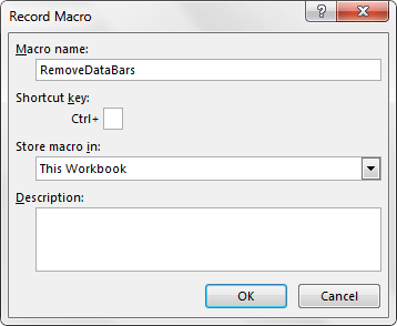
Figure 13-4: Start recording a new macro called RemoveDataBars.

3. Highlight cells C1:C21.

4. Go to the Home tab and select Conditional Formatting→Clear Rules→Clear Rules from Selected Cells.

5. Go to the Developer tab and click the Stop Recording command.

Excel stops recording.

You now have a new macro that removes conditional formatting rules from cells C1:C21.

Running your macros

To see your macros in action, follow these steps:

1. Select the Macros command from the Developer tab.

The dialog box in Figure 13-5 activates, allowing you to select the macro you want to run.

2. Select the AddDataBars macro.

3. Click the Run button.

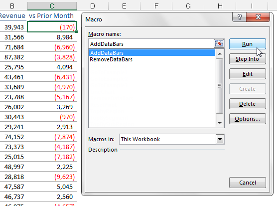
Figure 13-5: Use the Macro dialog box to select a macro and run it.

If all goes well, the AddDataBars macro plays back your actions to a T and applies the data bars as designed (see Figure 13-6).

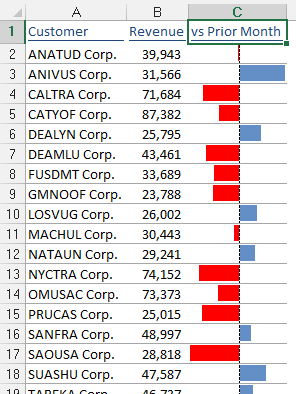
Figure 13-6: Your macro applied data bars automatically!

You can now call up the Macro dialog box again and test the RemoveDataBars macro shown in Figure 13-7.

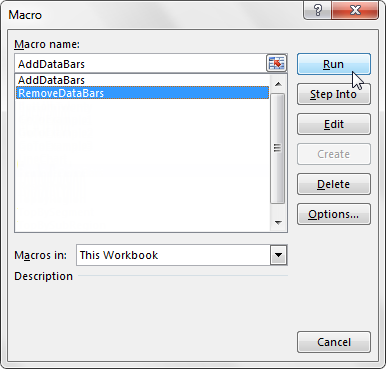
Figure 13-7: The RemoveDataBars macro will remove the applied data bars.

Assigning a macro to a button

When you create macros, you want to give your audience a clear and easy way to run each macro. A button, used directly in the dashboard or report, can provide a simple but effective UI.

Excel Form controls (refer to Chapter 12 for more information) enable you to create UI directly on your worksheets, simplifying work for your users. Form controls range from buttons (the most-commonly used control) to scroll bars and check boxes.

For a macro, you can place a Form control in a worksheet and then assign that macro to it — that is, a macro you’ve already recorded. When a macro is assigned to the control, that macro is executed, or played, each time the control is clicked.

Take a moment to create buttons for the two macros (AddDataBars and RemoveDataBars) you created earlier. Here’s how:

1. Click the Insert drop-down list under the Developer tab.

2. Select the Button Form control (see Figure 13-8).

3. Click the location you want to place your button. When you drop the button control into your worksheet, the Assign Macro dialog box, shown in Figure 13-9, opens and asks you to assign a macro to this button.

4. Select the macro that you want to assign. In this case, you can select the AddDataBars macro and then click OK.

5. Repeat Steps 1 through 4 for the RemoveDataBars macro.

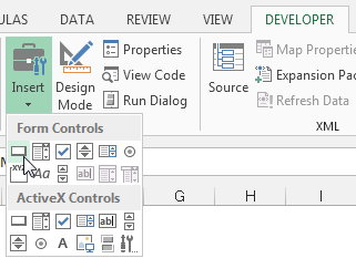
Figure 13-8: You can find the Form Controls in the Developer tab.

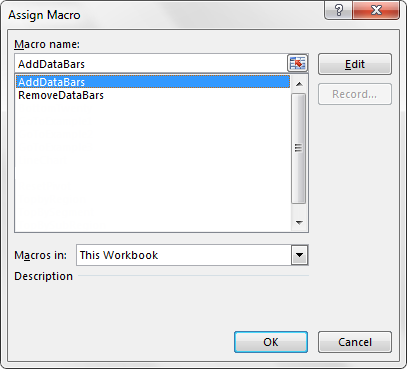
Figure 13-9: Assign a macro to the newly added button.

At this point, you have two buttons that run your macros. Keep in mind that all the controls in the Forms toolbar work the same way as the Command button — you assign a macro to run when the control is selected.

The buttons you create come with a default name, such as Button3. To rename your button, right-click the button and then select Edit Text.

Enabling Macros in Excel 2013

With the release of Office 2013, Microsoft introduced significant changes to its Office security model. One of the most significant changes is the concept of Trusted Documents. Without getting into the technical minutia, a Trusted Document is essentially a workbook you have deemed safe by enabling macros.

Viewing the new Excel security message

If you open a workbook that contains macros in Excel 2013, you’ll get a message in the form of a yellow bar under the Ribbon stating that Macros (active content) has, in effect, been disabled.

If you click Enable, the workbook automatically becomes a Trusted Document. This means you will no longer be prompted to enable the content as long as you open that file on your computer. The idea is that if you told Excel that you trust a particular workbook by enabling macros, it’s highly likely that you’ll enable macros each time you open it. Thus Excel remembers that you’ve enabled macros before and inhibits any further messages about macros (for that workbook).

This is great news for you and your clients. After enabling your macros just one time, they won’t be annoyed by the constant messages about macros, and you won’t have to worry that your macro-enabled dashboard will fall flat because macros have been disabled.

Setting up trusted locations

If the thought of any macro message coming up (even one time) unnerves you, you can set up a trusted location for your files. A trusted location is a directory that is deemed a safe zone where only trusted workbooks are placed. A trusted location allows you and your clients to run a macro-enabled workbook with no security restrictions as long as the workbook is in that location.

To set up a trusted location, follow these steps:

1. Select the Macro Security button on the Developer tab.

2. Click the Trusted Locations button.

This opens the Trusted Locations menu (see Figure 13-10). You see all the directories that Excel considers trusted.

3. Click the Add New Location button.

4. Click Browse to find and specify the directory that will be considered a trusted location.

Figure 13-10: The Trusted Locations menu allows you to add directories that are considered trusted.

After you specify a trusted location, all Excel files opened from this location will have macros automatically enabled. The idea is to have your clients specify a trusted location and use your Excel files from there.

Excel Macro Examples

Covering the fundamentals of building and using macros is one thing. Coming up with good ways to incorporate them into your reporting processes is another. Take a moment to review a few examples of how you can implement macros in your dashboards and reports.

Open the Chapter 13 Samples.xlsm file to follow along in the next section.

Building navigation buttons

The most common use of macros is navigation. Workbooks that have many worksheets or tabs can be frustrating to navigate. To help your audience, you can create some sort of switchboard, such as the one shown in Figure 13-11. When a user clicks the Example 1 button, he’s taken to the Example 1 sheet.

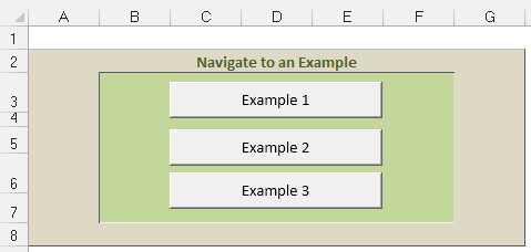
Figure 13-11: Use macros to build buttons that help users navigate your reports.

Creating a macro to navigate to a sheet is quite simple.

1. Start at the sheet that will become your switchboard or starting point.

2. Start recording a macro.

3. While recording, click the destination sheet (the sheet this macro will navigate to).

4. After you click in the destination sheet, stop recording the macro.

5. Assign the macro to a button.

Excel has a built-in hyperlink feature, allowing you to convert the contents of a cell into a hyperlink that links to another location. That location can be a separate Excel workbook, a website, or even another tab in the current workbook. Although using a hyperlink may be easier than setting up a macro, you can’t apply a hyperlink to Form controls (like buttons). Instead of a button, you use text to let users know where they’ll go when they click the link.

Dynamically rearranging pivot table data

In the example illustrated in Figure 13-12, macros allow a user to change the perspective of the chart simply by selecting any one of the buttons shown.

For more information about pivot tables, see Chapter 14. For more information about pivot charts, see to Chapter 15.

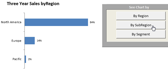
Figure 13-12: This report allows users to choose their perspective.

Figure 13-13 reveals that the chart is actually a pivot chart tied to a pivot table. The recorded macros assigned to each button are doing nothing more than rearranging the pivot table to slice the data using various pivot fields.

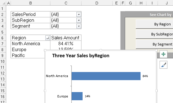
Figure 13-13: The macros behind these buttons rearrange the data fields in a pivot table.

Here are the high-level steps needed to create this type of setup:

1. Create your pivot table and a pivot chart.

2. Start recording a macro.

3. While recording, move a pivot field from one area of the pivot table to the other. When you’re done, stop recording the macro.

4. Record another macro to move the data field back to its original position.

5. After both macros are set up, assign each one to a separate button.

You can fire your new macros in turn to see your pivot field dynamically move back and forth.

Offering one-touch reporting options

The last two examples demonstrate that you can record any action that you find of value. That is, if you think users would appreciate a certain feature being automated for them, why not record a macro to do so?

In Figure 13-14, notice that you can filter the pivot table for the top or bottom 20 customers. Because the steps to filter a pivot table for the top and bottom 20 have been recorded, anyone can get the benefit of this functionality without knowing how to do it themselves. Also, recording specific actions allows you to manage risk a bit. That is, you’ll know that your users will interact with your reports in a method that has been developed and tested by you.

This not only saves them time and effort but it also allows users who don’t know how to take these actions to benefit from them.

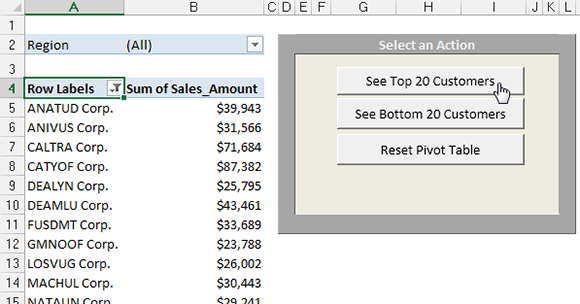
Figure 13-14: Offering prerecorded views saves time and effort and allows users who don’t know how to use advanced features to benefit from them.

Feel free to visit Chapter 14 for a refresher on how to create the top and bottom reports you see in Figure 13-14.

Figure 13-15 demonstrates how you can give your audience a quick-and-easy way to see the same data on different charts. Don’t laugh too quickly at the uselessness of this example. It’s not uncommon to be asked to see the same data in different ways. Instead of taking up real estate, just record a macro that changes the Chart Type of the chart. Your clients will be able to switch views to their hearts’ content.

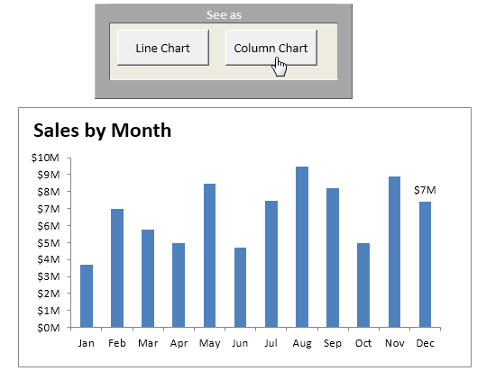
Figure 13-15: You can give your audience a choice in how they view data.