B.1 DIMENSIONING

In order to understand the geometric dimensioning and tolerancing system, we must first understand the appropriate method for dimensioning or putting dimensions on a drawing. Dimension placement, symbols, and conventions are all important to the common language for engineers and machinists. The following concepts are essential for understanding dimensioning of technical drawings.

B.1.1 Orthographic Views

Most technical drawings show orthographic views of the object being represented. Orthographic or principal views are drawings based on the projection of the object onto a plane. The best way to visualize an orthographic drawing is to imagine a “glass box” around the object, with a projection of the object onto each surface of the box. The box is then unfolded to give rise to the six primary views of the orthographic drawing: top, front, and bottom views; and right-side, left-side, and rear views (Figure B.1). It should be noted that this particular type of orthographic drawing uses third angle projection in which the drawing is derived from an image projected onto a plane between the observer and the object, so that the order is observer, projected view, object. Or, said somewhat differently, in third angle projection the image is projected onto a plane in front of the object.

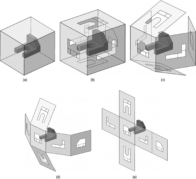
FIGURE B.1 The six orthographic or principal views of an object. The orthographic views are created by projecting the object onto a plane. This can be visualized by imagining: (a) a “glass box” around an object; with (b) a projection of the object onto each face; and then (c–e) the unfolding of the box leads to the six views: front, top, bottom, right side, left side, and back views. Note that in practice, we often need to use only the front, top, and right side views to fully describe the object as the others are redundant. Adapted from Engineering Graphics Essentials by permission of K. Plantenberg.

FIGURE B.2 First and third angle projections. The difference between these two orthographic projections lies in the location of the plane on which the object is projected. In first angle projection, the object is projected onto a plane behind it. In third angle projection, the object is projected onto a plane in front of it. Note the different symbols used to represent each drawing type. Reprinted from ASME Y14.3-1975 and ASME Y14.5-1994 (R2004), by permission of The American Society of Mechanical Engineers. All rights reserved.

In Japan and some European countries, a different type of orthographic view is used: In first angle projection the drawing is derived from an image projected onto a plane behind the object, so that the order is observer, object, projected view. That is, in first angle projection the image is projected onto a plane behind the object. The two types of orthographic views can lead to very different drawings and it is important to know which system is being used. Figure B.2 shows the views in first and third angle projections, as well as the symbols used to denote which system is depicted. It is important to note that all six views of the orthographic projection are not always required. We can often fully define an object with front, top, and right-side views (in third angle projection), or front, bottom, and right side (in first angle projection). In some cases we need only the front and top views. It is important to note that the orthographic views are to be laid out as one drawing, that is, the three (or two) views must line up as they are laid out in the projection, with features aligning in the views.

Choosing an appropriate front view for an orthographic drawing is essential for ensuring its correct interpretation. It is much easier to figure out what is being represented given the right front view, because that front view is seen first and it represents the most basic and characteristic profile of the object being drawn. In addition, the front view should be stable (i.e., heavy on the bottom), and should have as few hidden lines as possible. Consider a block letter “E,” as in Figure B.3. Several poor choices for front views of this object are shown, as well as several “best” front views.

FIGURE B.3 Choosing a front view: (a) isometric view of object to be drawn; (b) front view should be chosen to show the most informative profile of the object; (c) the front view should be chosen so that the view shows the most stable version of the object; (d) a front view should be chosen to minimize the hidden lines of an object in other views; and (e) the best choice of views for this object: front and top views.

B.1.2 Metric versus Inch Dimensioning

Metric and inch dimensions (and that is what they're called) are specified differently in the ASME standard, which enables us to tell at first glance which system of units is used on a drawing. American (inch or in.) dimensions are specified to have no zero before the decimal point (e.g., .5 in.). Further, the dimension must contain the same number of decimal places as the tolerance for that dimension. For example, if the tolerance for a given dimension is .01 in., the dimension must be .50 in. Metric dimensions include a zero before the decimal point (e.g., 0.5 m). A metric dimension does not need to match the number of decimal places with the tolerance, and no decimal point or zero is included if the dimension is a whole number.

B.1.3 Line Types

Technical drawings use several different types of lines. The weight and style of these lines, as well as their placement on the drawings, are specified in the ASME standard. Most CADD packages include settings for the ASME standard, so that they will automatically place the lines correctly if they are initially set correctly. Extension lines come out from a part and leave a visible gap between the part and the line. Examples of extension lines can be seen in Figure B.4; these are the vertical lines up from the screwdriver handle. Dimension lines are typically broken for the numbers and are placed at least 10 mm apart from the object on the drawing. Subsequent dimension lines are at least 6 mm apart. Examples of these lines can also be seen in Figure B.5. Leader lines are used to indicate surfaces and hole diameters. They should be at an angle between 30 and 60°, point toward the center of a hole, and include only one dimension per leader line. The left-side view of the screwdriver print shows a leader line pointing to the outer diameter of the piece; note that the arrow points directly at the center of the diameter. Hidden lines are dashed lines (- - - - - - - -) that indicate the presence of a feature that is seen in another view. Hidden lines indicate the presence of a hole in the object shown in Figure B.4. The front view shows the hole; the side view uses hidden lines to indicate where the hole is located. Center lines are used to indicate a cylinder and are represented by the type of dashed line shown in Figure B.5. The presence of this type of line alone indicates a cylindrical feature; the side view showing the part is a cylinder is not needed.

FIGURE B.4 A drawing of a screwdriver blade indicates all the types of dimensions: basic (indicated by boxing of the numbers); reference (indicated by parentheses); stock (indicated by STOCK following the dimension); and size/location dimensions (for example, the overall blade length, 5.00 in.). Courtesy of R. Erik Spjut.

FIGURE B.5 Hidden lines are indicated by dashed lines. They are used to represent a feature in a view where that feature is not explicitly seen. For example, the hole shown in the front view is located by hidden lines in the side view.

B.1.4 Orienting, Spacing, and Placing Dimensions

The most common practice is to orient all dimensions such that they can be read when the drawing is held horizontally. It is also acceptable to use an aligned system in which dimensions are oriented either vertically such that they can be read from the right or horizontally such that they can be read from the bottom. As mentioned before, the minimum spacing between adjacent dimensions is specified as 6 mm. The placement of dimensions is also important. Dimensions should be stacked with the shortest dimensions placed closest to the object and longer dimensions beyond them. This system avoids crossing extension lines, thereby minimizing confusion. Dimensions should also be staggered to make it easier to read them. In addition, in orthographic drawing views, the dimensions should be placed between the drawings views, that is, between the front and top views, and between the front and right-side views. The overall size, length, height, and depth should be specified.

B.1.5 Types of Dimensions

It is important to distinguish between size dimensions and location dimensions. Size dimensions define the size of features: overall height, length, thickness, diameter of a hole, size of a slot, and so on. Location dimensions specify where a feature is located with respect to other features or the edge of an object. Location dimensions define the center of a hole or the location of a slot, for example, with respect to the edge of a part or with respect to another feature. The general rule of thumb is to dimension size dimensions first, then do location dimensions. Remember that both size and location dimensions will have tolerances associated with them, a concept that we will revisit later in this chapter.

In addition to size and location dimensions, there are three other dimension types that are important: basic dimensions, reference dimensions, and stock dimensions. Figure B.6 is a drawing of a screwdriver blade, from the same screwdriver whose handle appears in Figure B.5, and it illustrates all of these types of dimensions. (And by the way, are the dimensions in this drawing in millimeters or inches?) First, the overall blade length in Figure B.6 is an example of the size dimensions above. The boxed numbers in the drawing are basic dimensions (e.g., the .250 dimension from the blade end to the hole on the left side of the drawing). Basic dimensions define the basis for permissible variation, or tolerance, in the geometric dimensioning and tolerancing system. In other words, they define the theoretically exact point from the end of the blade from which to measure the variation in the location of the hole. We will revisit this concept in the next section on tolerancing. Reference dimensions are indicated in parentheses, for example, the (1.00) dimension on the screwdriver blade in the top view. A reference dimension is a point of information for the machinist and is not a requirement. It means that if the part has been produced correctly, the blade length should be around 1 in. The last type of dimension is a stock dimension, and it is indicated by writing .25 STOCK on the drawing. This indicates that the material used for the part comes from the manufacturer with a specified size and associated tolerance; no further tolerance specification is required.

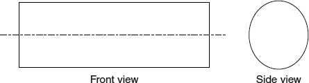
FIGURE B.6 Center lines are indicated by a different type of dashed line and describe cylindrical features.

Every specified dimension requires an associated tolerance in a technical drawing except basic, reference, and stock dimensions. This makes sense when we realize the purpose of these types of dimensions. One more important note should be made: Any number on a technical drawing that does not have a tolerance directly associated with it (e.g., .50 ± .01), still has a specified tolerance on the drawing. These tolerances are specified in the title block of a technical drawing and are called block tolerances. In Figure B.6 the block tolerances can be seen to be .XX ± .03. The tolerance is determined by the number of decimal places in the dimension. This means that the 5.00 overall blade length has a tolerance of ±.03 in.

B.1.6 Some Best Practices of Dimensioning

Each of the concepts and dimension types described above can be integrated into a set of guidelines for dimensioning a technical drawing. Three of the most important rules for dimensioning are as follows:

• Dimension the size dimensions first, then do the location dimensions.
• Do not double dimension. In an orthographic drawing, it is not necessary to specify the same dimension twice. For example, specifying the depth of an object on the right and top views leads to unnecessary clutter in the drawing. It is not good drawing practice.
• Do not dimension to hidden lines. Dimension a feature where it is visible. A hole, for example, should be dimensioned in the view where it is visible. This is good practice that leads to clearer technical drawings.

B.2 GEOMETRIC TOLERANCING

Now that we have covered some basic dimensioning symbols and rules, we turn to geometric tolerancing. A tolerance is the permissible variation of a part. Tolerances are applied to all size and location dimensions. Tolerances are required because we, as engineers, need to know how much a part can vary from its specifications before it no longer functions as intended. Defining tolerances requires that we know and understand the function of a given part. It is good practice to specify tolerances only as tightly as we need because parts become much more expensive to manufacture as their tolerances become smaller. Figure B.7 shows the relative cost of increased tolerances. Here the y-axis tracks the percentage of increase in cost of making the hole, and the x-axis shows both the size and location tolerances on the hole. (Location tolerances will be described below.) This figure not only gives us an idea of the increased cost as the tolerances become tighter, but also tells us what type of machinery is required to make such a hole. It is not surprising that the more precise a hole it can make, the more expensive the equipment!

FIGURE B.7 Relative cost of manufacturing as hole location tolerance gets smaller. The cost goes up significantly as smallertolerances are prescribed. In addition, special equipment is required to meet tight tolerances. Reprinted by permission of Technical Documentation Consultants of Arizona, Inc.

All dimensions require a tolerance (except for the basic, reference, or stock dimensions described above). On a drawing, there are several places to look for tolerance specifications:

• associated with a dimension (+/−);
• in a feature control frame (which we describe below);
• in a drawing note; or
• in the block tolerance as the default if no other tolerance is applied.

It is possible to tolerance every dimension with a plus or minus tolerance, but the geometric dimensioning and tolerancing system provides more leeway for each part, which in turn leads to cost savings. The geometric tolerancing system takes into account not only variations in size of an object, but also permissible variations on the position, form, and orientation of features. We now describe some of the tolerancing components of the GD&T system.

B.2.1 The 14 Geometric Tolerances

There are 14 characteristics specified in the ASME Y14.5M-1994 standard that can vary, and therefore have an associated tolerance (Figure B.8). For example, we can specify how much a surface can vary in flatness or how much variation is permissible in the location of a hole. These 14 characteristics are categorized into five groups: form, profile, orientation, location, and runout. These groups are somewhat hierarchical. For example, a position tolerance is a refinement of an orientation tolerance, which is a refinement of a form tolerance, which is a refinement of the size tolerance on a feature. For example, if a rectangular piece is .500 ± .004 in. in height, the minimum height is .496 and the maximum is .504, simply based upon the size dimensions. If each end of the part was made at one of these extremes—the part would be within the size tolerance—the maximum out-of-flatness that the top surface could be is .008. Therefore, if a flatness tolerance is to be applied to this part, it must be less than .008 in. for it to make sense.

Form tolerances apply to individual features, for example, a surface in the case of straightness or flatness. All other tolerances apply to related features. For example, orientation and location tolerances specify permissible variation of a given feature with respect to a reference frame. Therefore, these tolerances require specification of a reference frame in order for them to be meaningful. The reference frames are defined by datums, which we will soon discuss below.

A full discussion of all of the 14 geometric tolerances is beyond our scope (see the notes in Section .4 for further reading). Therefore, we will focus specifically on position tolerances to show how geometric tolerances are applied.

B.2.2 Feature Control Frames

Feature control frames are devices used to specify the particular geometric tolerance on the technical drawing. We have seen them in the drawings presented earlier. The feature control frame is attached to a surface via a leader line (e.g., the flatness tolerance associated with the screwdriver blade in the top view in Figure B.6); placed off of an extension line from a surface (e.g., the flatness and perpendicularity tolerances associated with the tip of the blade in the front view in Figure B.6); or associated with the size dimension of a particular feature (e.g., the position tolerances on the hole in the top view of Figure B.6).

FIGURE B.8 The 14 geometric tolerances and their symbols. Reprinted from ASME Y14.3-1975 and ASME Y14.5-1994 (R2004), by permission of The American Society of Mechanical Engineers. All rights reserved.

The feature control frame is broken down into the three components depicted in Figure B.9. We will define the parts from left to right. The first box (1) is for the geometric characteristic symbol, which tells us what tolerance is being specified. In this case, it is position.

The second box (2) contains the actual permitted variation, or tolerance with some optional modifiers. In this particular case, the tolerance is .014 in. The diameter symbol in front of the number indicates that the tolerance zone shape is cylindrical. Figure B.10 indicates the difference between the presence and absence of a diameter symbol in defining a tolerance zone shape. A position tolerance with a diameter symbol means that the position of the item being controlled must fit inside a cylindrical tolerance zone of a diameter specified by the tolerance. Lack of a diameter symbol indicates that the position must fall between two parallel planes; the distance between those planes is defined by the tolerance specified. The tolerance material condition modifier appears after the tolerance itself and specifies the conditions under which this tolerance applies. Material condition modifiers will be described fully below.

FIGURE B.9 A feature control frame for an object that specifies the position of that object to a cylindrical tolerance zone of 0.014 in. with respect to a reference frame determined by datums A, B, and C.

The last set of boxes (3) contains the datum references. These define the frame of reference from which the tolerance is measured. The datum references appear in a specific order that indicates their relative importance. Note that datum references may also have material condition modifiers (described immediately below).

The feature control frame described in Figure B.9 can be read as follows, assuming it is associated with the size dimension for a hole: The hole has a permissible variation in position such that the center of the hole must fit within a cylindrical tolerance zone that is .014 in. in diameter when the hole is at maximum material condition (MMC), with respect to datums A, then B, then C.

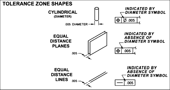
FIGURE B.10 The tolerance zone shape depends on the type of tolerance being specified and the presence or absence of a diameter symbol before the tolerance in the feature control frame. Reprinted by permission of Technical Documentation Consultants of Arizona, Inc.

B.2.3 Material Condition Modifiers

Three material condition modifiers specify the state of the feature when the tolerance is applied. These are: maximum material condition, least material condition (LMC), and regardless of feature size (RFS). It is important to know under what conditions the part is toleranced, because use of these modifiers can lead to substantial cost savings.

Maximum material condition is the condition in which a feature of size contains the maximum amount of material (weighs the most) within its size tolerance. MMC is indicated by the letter M enclosed in a circle, as in Figure B.9. For a hole, this means the minimum diameter specified in the size tolerance. For a cylindrical shaft, this means the maximum diameter specified by the size tolerance. For example, a hole specified as .500 ± .005 in. in diameter would have an MMC size of .495 in. in diameter.

Least material condition, indicated by the letter L enclosed in a circle, is the condition in which a feature of size contains the least amount of material (weighs the least) within its size tolerance. The LMC size of the hole is the largest hole within the size tolerance; the LMC size of a shaft is the smallest shaft within the size tolerance. The same hole described above would have an LMC size of .505 in.

Regardless of feature size means just that the tolerance is applied regardless of the size of the produced part. It is indicated by the absence of either MMC or LMC modifiers.

Why would we want to use these modifiers? These modifiers are extremely useful in that they can reduce the cost of manufacturing a part substantially. They take into account the fact that if a part is produced at the extremes of its permitted size variation, there is potential for more “wiggle room” in the placement of that part. For example, if a hole is produced at its largest possible size, its position can vary more than it would if it was produced at its smallest possible size—and still match up with a mating part. The material condition modifiers enable us to have a maximum interchangeability of parts. This is important if we are trying to manufacture thousands of the same pieces, and we expect them all to fit together without specifying extremely tight tolerances.

If a maximum material condition modifier is placed in a feature control frame associated with the tolerance, this means that the specified tolerance applies only at the MMC size of the feature. Figure B.11 shows a part with two holes controlled by a position tolerance. Since this tolerance is specified at MMC, it means that when the hole is produced at its MMC size (smallest hole, .514 in. this example), the center of the hole must fit within a cylindrical tolerance zone of diameter .014. If however, the hole is produced larger than the MMC size, additional bonus tolerance is added to the allowable position variation. The bonus tolerance added is the difference between the MMC size of the hole and the actual size of the hole. This bonus tolerance is to account for the fact that a larger hole can vary more and still line up with a mating part. Essentially, it takes into account the additive effects of the variation in size and variation in position.

We illustrate the use of a least material condition modifier in Figure B.12. The same example is shown, this time with the tolerance specified at LMC instead of MMC. In this case, when the hole is produced at its largest size, .520, the tolerance is specified as .014. As the hole gets smaller, bonus tolerance is added to allow the hole to vary more in position. The LMC modifier is used less than the MMC modifier but is useful when it is desirable that the position of a larger hole needs to be more tightly controlled, such as in the case where it is placed near the edge of a part.

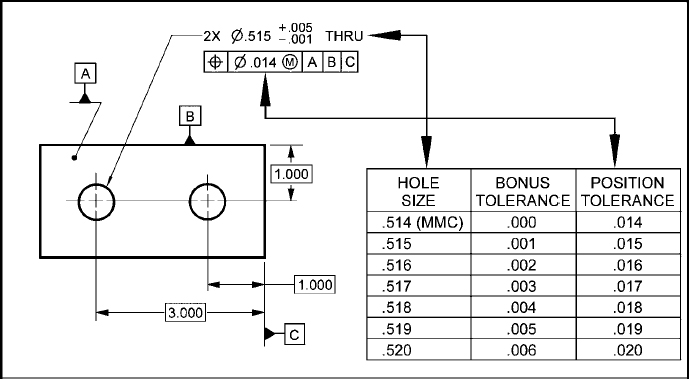
FIGURE B.11 Maximum material condition modifier allows additional “bonus tolerance” if part is produced at a size other than MMC. In this example, as the produced hole gets larger, the allowable variation in its position also gets larger. Reprinted by permission of Technical Documentation Consultants of Arizona, Inc.

FIGURE B.12 Least material condition modifier applies the tolerance in the case of least material condition and allows bonus tolerance for parts produced (in the case of a hole) smaller than the LMC size. This modifier is used much less frequently than the MMC modifier and can help to control hole position if the hole is located close to the edge of a part. Reprinted by permission of Technical Documentation Consultants of Arizona, Inc.

RFS does not take advantage of size variations in the feature and specifies the same tolerance for all cases. This condition is assumed if no material condition modifier is used on the drawing, so we should be careful not to omit these symbols! RFS should be used only if the requirements are very strict, since manufacturing parts to RFS is much more expensive.

One final note on material condition modifiers. These conditions may only be applied to features of size. A feature of size can be a cylinder, a slot, or a hole, for example. Material condition modifiers may not be used applied to surfaces, as there is no size associated with a surface. It wouldn't make sense, therefore, to have a material condition modifier associated with a tolerance in a flatness feature control frame applied to a surface.

B.2.4 Datums

As we mentioned earlier, in the GD&T system datums form the reference frame from which to locate tolerance zones specified in the feature control frames. A few definitions are in order before we proceed. A datum symbol is used to define the datum on the drawing. A datum symbol looks like this:

Any letter, but for I and Q, may be used as a datum symbol. We must be careful about where we place the datum symbol because we want to be sure that the correct feature is specified as the datum. To specify a surface as a datum, the datum symbol may be placed off of an extension line or may be attached directly to the surface itself (Figure B.13). To specify a feature of size as a datum, the datum symbol may be placed in line with the dimension line for the feature, or it may be attached directly to a cylindrical feature in the view where it appears as a cylinder. Datum symbols may also be attached to the feature control frame associated with the feature of size (see Figure B.14).

A datum feature is what the datum symbol is applied to, the actual feature on the part. A datum simulator is the manufacturing and inspection tooling used to simulate the datum during production. Simulators can be a precise surface or precise tooling in which to place the part. Locations of holes or other features are then determined from the datum simulator instead of the irregular surface or edge of the part itself. The datum simulator for a surface is a surface that the part may be placed upon, and is typically made from granite due to its smooth surface free of irregularities. The simulator for a feature of size is usually a chuck or a vice that clamps around an external feature.

So how do we choose the datums for a particular part? Considerations should include the function of the part, the manufacturing processes to be employed, inspection processes that may be used, and the part's relationship to other parts. For a rectangular object, three datum references must be chosen to refer to three perpendicular planes (see Figure B.15). The primary datum (A) is listed first in the feature control frame and must make three points of contact on that surface. If our rectangular part is going to fit flush with another part, the largest contacting surface should be chosen as the primary datum. The primary datum creates a flat surface. The secondary datum (B) is usually the longest side, or a side in contact with a mating part, and requires two points of contact. This datum creates alignment and stability. The tertiary datum (C) is, then, the other side of the part. This datum requires one point of contact and prevents the part from sliding on datum B. In order to measure the accuracy of a part for testing, or to machine a hole located with respect to these datums, the part must first be set down on datum A, slid over to make contact with datum B, and then slid until it makes contact with datum C, while maintaining contact with datums A and B.

FIGURE B.13 Specifying surfaces as datum features. The datum symbol may be placed directly on the surface or off an extension line from the surface. The datum symbol must be separated from the dimension line. Courtesy of Elizabeth J. Orwin in SolidWorks™.

For a cylindrical object, two datum references are required (see Figure B.16) One reference is the surface, the other is the axis determined by a particular feature of size. In Figure B.16, the primary datum D is the bottom surface; it establishes a flat surface with three points of contact. The secondary datum E is established by the axis of the cylindrical part. This axis establishes two planes that bisect at the axis. To measure or locate from this datum, the part must be contacted by a chuck at three points. To make this particular part, the cylinder would be placed on a precise surface, and grabbed by a chuck to establish the axis, and then the holes would be located from there.

Many parts have large irregular surfaces that are not flat surfaces and not cylindrical parts. For these parts, it is impractical to define datums as we have described above. In these cases, it is permissible to identify datums using points, lines or areas instead of a whole surface. These points are called datum targets and specify where the workpiece contacts the tooling during manufacturing and inspection. A datum target is indicated by an “X” on the drawings, and the datum reference symbols are defined in circles. Since a whole surface is not in contact, the points of contact are typically numbered “A1,” “A2,” and so on. Figure B.17 shows a hammer handle from Harvey Mudd's introductory engineering design course with X's marking the datum targets on this irregularly shaped handle surface. The profile of the surface is then permitted to vary with respect to those points.

FIGURE B.14 Specifying features of size (such as holes or shafts) as datum features. The datum symbol may be placed in line with the size dimension of the feature, placed on the feature itself, or associated with the feature control frame. All the datum symbols on this drawing indicate the .250 diameter cylindrical shaft as the datum. Courtesy of Elizabeth J. Orwin in SolidWorks™.

One last note on datums and datum references. It is important to understand that not all types of tolerance specifications require a datum reference. (Recall that we showed all of the geometric tolerances in Figure B.8.) Note that the first set of tolerances are form tolerances and apply to individual features. The column on the far left in the figure distinguishes the tolerances that apply to individual features versus ones that apply to related features. For example, a flatness tolerance is applied to a surface: That surface is specified to be flat, but it is not with respect to any frame of reference. It would be inappropriate to specify a datum reference in this case. In contrast, a perpendicularity tolerance specifies that some feature be perpendicular to something; this something must be defined by one or more datum references.

FIGURE B.15 Specifying datums for a rectangular feature. The function of the part is important for specifying datums. The primary datum is usually chosen as the largest contacting surface. Reprinted from ASME Y14.3-1975 and ASME Y14.5-1994 (R2004), by permission of The American Society of Mechanical Engineers. All rights reserved.

B.2.5 Position Tolerance

We have used position tolerance examples throughout the foregoing discussion, and we will now put the pieces together using the illustrative example shown in Figure B.18. The part depicted in this drawing has a specified position tolerance on the hole. The specified tolerance defines a cylindrical tolerance zone (note the diameter symbol) .100 in. in diameter that extends through the part. The hole axis may be tilted, but it must fit within that tolerance zone. Since MMC is specified, this tolerance is required to be met at MMC only, that is, at the smallest hole size. As the hole gets larger, bonus tolerance is added, making the cylindrical tolerance zone for the hole axis larger as the hole gets larger. The theoretical center of the hole is located at specified distances from the datums; these specified distances are called out using basic dimensions (boxed). To make this part, the stock piece would be placed on a datum simulator surface (datum A), pushed up against datum simulator surface B, and slid along to make contact with datum simulator surface C. The theoretical center of the hole would then be located from the datum simulators surfaces B and C using the basic dimensions on the drawing. Any drawing that has tolerances specified by a feature control frame will have basic dimensions defining distances between the datums and the theoretical position of the tolerance zone.

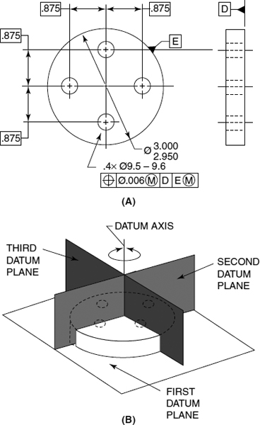
FIGURE B.16 Specifying datums for a cylindrical feature. The primary datum is usually chosen as the flat surface to stabilize the part. The secondary datum is the axis described by the cylindrical feature. Reprinted from ASME Y14.3-1975 and ASME Y14.5-1994 (R2004), by permission of The American Society of Mechanical Engineers. All rights reserved.

B.2.6 Fasteners

How do we know how to specify position tolerance zones such that we can fasten two parts together? How do we ensure that fasteners will always fit? There are three types of fastener conditions:

• Floating fasteners: The fasteners pass through holes on two or more parts and are fastened with a nut on the other side. The fasteners do not need to come into contact with the part.

FIGURE B.17 A drawing of the hammer handle. Note the use of datum targets (marked as “X's” on the drawing) instead of a datum feature. Courtesy of R. Erik Spjut.

• Fixed fasteners: One of the two (or more) parts involved is tapped or press fit (fixed) and the other has a clearance hole. The fixed part fixes the location of the fastener.
• A double fixed fastener: Here both holes are fixed. This gives zero position tolerance at RFS and should be avoided due to expense.

How do we calculate the position tolerance of any given hole in two parts that are to be fastened together? For a floating fastener condition, we first determine the MMC size of the hole (smallest hole, H) and the MMC size of the fastener (largest fastener, F). The difference between these two numbers gives the amount of clearance available in the worst-case scenario, when both fastener and hole are at MMC. The amount of tolerance in this case is simply this difference, that is, the tolerance T = H − F. For a floating fastener condition, this tolerance is applied to the position of the holes on both parts. For a fixed fastener condition, the tolerance is calculated in the same way, but now the tolerance must be distributed over the two parts. The rule of thumb is to give 60–70% of the allowable tolerance to the fixed/threaded part.

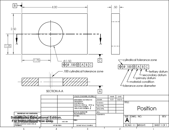
FIGURE B.18 Putting it all together: tolerancing the true position. Courtesy of Elizabeth J. Orwin in SolidWorks™.

B.3 HOW DO I KNOW MY PART MEETS THE SPECIFICATIONS IN MY DRAWING?

All manufactured parts need to be evaluated to make sure that they are within the specifications. A coordinate measurement machine (CMM) is a device that can be programmed to examine a specific part for its adherence to the geometric tolerances specified on the drawings. Often companies will invest in one of these systems if they are manufacturing a large number of similar parts and need to know if each part meets the requirements. Figure B.19 is a photograph of the hammer, described in the technical drawing in Figure B.17, mounted on the CMM system at HMC. Note that the points at which the tooling makes contact with the hammer correspond to the datum target points we saw in the drawing. This system is used to grade student-machined tools at HMC, but is more widely used in industry for quality control of manufactured parts.

There is another, much cheaper, way of evaluating parts that fit together called functional gaging. As the name hints, this method evaluates the function of a given part, that is, will a part fit with its intended mating part? This approach further illustrates the power of the material condition modifiers. In order to understand functional gaging, we must first define another term: The virtual condition of a given feature is the combined effect of the size tolerance and the geometric tolerance on the part. If we imagine an external feature, such as a cylindrical shaft, the virtual condition is the MMC size of the shaft plus the geometric tolerance. It is the largest possible shaft with the largest possible variation in position, making it the worst-case scenario for the external part fitting into a mating part. For an internal feature, such as a hole, the virtual condition is also the worst-case scenario, the MMC size of the hole (smallest hole) minus the geometric tolerance. The virtual conditions of the two parts must match in order to ensure that two parts, specified on different drawings and manufactured to specifications, will always fit together. If the virtual condition of a hole in one part is matched to the virtual condition of a shaft in another part meant to fit together, this will ensure maximum interchangeability of parts. The result is powerful. It means that all parts that meet the drawing specifications will be interchangeable, that is, the two parts need not be made specifically to fit together. This clearly offers large cost savings in the manufacturing of parts.

FIGURE B.19 The hammer described by the drawing in Figure B.17 on the coordinate measurement machine. Note the ruby tip used to measure the part and the precise granite surface of the machine. Note also that the tooling used to hold the hammer while it is being tested make contact with the part at the datum target locations specified in the drawing.

Now, back to functional gaging. Virtual condition matching allows us to use this much cheaper way to evaluate manufactured parts. In our hole/shaft example above, we could simply manufacture one part with the shaft made at virtual condition and then use that part to evaluate the potentially hundreds of matching parts. The manufactured part with the hole to be tested would simply be placed over the shaft at virtual condition: If the hole goes over the shaft, the part is good; if not, the part is thrown out.

B.4 NOTES

Section B.1: Our brief overview of the basics of dimensioning and tolerancing has relied on the information found in ASME (1994), TDCA (1996), Plantenberg (2010), and Wilson (2005).