
CHAPTER OBJECTIVES
To explain demand and supply, and show how they work using schedules and graphs.
To show how demand and supply are affected by changes in price and nonprice factors.
To demonstrate how demand and supply interact in markets to determine prices, and to show equilibrium price and quantity, shortages, and surpluses in a market.
To explain how changes in demand and changes in supply affect equilibrium prices and quantities in markets.
To illustrate how government-imposed price ceilings and price floors influence market conditions.
To introduce the concept and calculation of price elasticity, which measures buyers' and sellers' sensitivities to price changes.

As we noted in Chapter 2, one way societies can make the basic economic decisions is through individual buyers' and sellers' actions in markets. Many societies, such as the United States, and some countries in Western Europe and Asia, base their economic systems on such market decision making. There are two basic economic tools to study buyers and sellers and their behaviors in the marketplace: demand and supply. Together, these tools help us understand the forces at work in a market economy. In this chapter, we explore demand and supply in detail, and then put the two together to see how they interact to determine the prices of goods and services.
DEMAND AND SUPPLY
Demand: The Buyer's Side
Demand, in economic terms, refers to buyers' plans concerning the purchase of a good or service. For example, you might demand an airplane ticket to London, tennis lessons, or a chemistry lab book. A business might demand workers, raw materials, machinery, or any other factor of production. Many considerations go into determining the demand for a good or service. These include the product's price as well as nonprice factors such as the buyer's income and attitude toward the item and available substitute products.
Demand, Defined In formal terms, we define a buyer's demand for a good or service as the different amounts of the good or service that the buyer would be willing and able to purchase at different prices over a given period of time with all nonprice factors held constant. Therefore, when we speak of a buyer's demand for baseball tickets, gasoline, or whatever, we are speaking of the different amounts of the item that the buyer would purchase at different prices over some period of time, such as a day, a week, or a year, with all nonprice factors unchanged. In determining demand, note that only the product's price is allowed to change: All nonprice factors that affect demand, such as the buyer's income, are held constant in order to highlight the relationship between the product's price and the amount of the product a person would be willing and able to buy.
Demand
The different amounts of a product that a buyer would purchase at different prices in a defined time period when all nonprice factors are held constant.
We can illustrate the relationship between the amount of a product that a consumer would buy and the product's price in two ways: through a demand schedule (or table) and through a graph (called a demand curve). Table 3.1 is a demand schedule that shows Zach's weekly demand for fresh-baked bagels.1 Note the relationship between the price per bagel and the number of bagels that Zach is willing and able to buy. As the price per bagel goes up from $0.20 to $0.40, the number of bagels Zach would buy falls from 15 to 12; as the price increases from $0.40 to $0.60, the amount demanded falls from 12 to 10. Each additional $0.20 increment further reduces the number of bagels Zach would buy. In other words, as the price increases, Zach would buy fewer fresh-baked bagels. We could have used any other consumer and any other good or service—restaurant meals, plastic pink flamingos, digital cameras, or jeans—with the same result: The quantity demanded falls as the price rises, and the quantity demanded rises as the price falls.
Demand Schedule
A list of the amounts of a product that a buyer would purchase at different prices in a defined time period when all nonprice factors are held constant.
Law of Demand Zach's buying behavior, illustrated in Table 3.1, reflects a typical buyer's plan to purchase a good or service. It shows a relationship between price and quantity demanded that we know to be generally true. This relationship is called the Law of Demand. It states that, holding all nonprice factors constant, as a product's price increases, the quantity of the product demanded decreases, and as a product's price decreases, the quantity demanded increases. In other words, the Law of Demand states that a product's price is inversely related to the quantity of that product that consumers demand.
Law of Demand
There is an inverse relationship between the price of a product and the quantity demanded.
TABLE 3.1 Zach's Weekly Demand for Fresh-Baked Bagels
This demand schedule lists different amounts of bagels that Zach would purchase each week at various prices and illustrates the Law of Demand: It shows the inverse relationship between price and quantity demanded.
| Price per Bagel | Number of Bagels Demanded Weekly |
| $0.20 | 15 |
| 0.40 | 12 |
| 0.60 | 10 |
| 0.80 | 8 |
| 1.00 | 6 |
| 1.20 | 4 |
| 1.40 | 2 |
| 1.60 | 1 |
Why do consumers react this way to price changes? Behind the Law of Demand is the fundamental problem of economics: scarcity and choice. Consumers purchasing goods and services face a scarcity problem: Their incomes are always limited. Consumers—even very wealthy consumers—can afford only so much. So as the price of an item goes up, buyers may not be able to afford as much of it as they could at the lower price. On the other hand, when the price of a good or service falls, consumers will likely increase their purchases of the item because they can satisfy more wants and needs with their limited incomes.
Choice also influences demand because consumers can always purchase alternative (or substitute) products. As the price of fresh-baked bagels increases, Zach can choose to eat other foods—doughnuts, cereal, or fruit, to name a few—in place of bagels. As the price of bagels decreases, he may choose to eat more of them and less of other items.
Graphing Demand Typically, economists display demand in graphs rather than in schedules or tables. Figure 3.1 shows Zach's demand for bagels exactly as it appeared in Table 3.1, but presented graphically. On this graph, price appears on the vertical axis (measured in 20-cent intervals) and quantity demanded appears on the horizontal axis (in two-bagel increments). When we plot each price–quantity combination from the demand schedule in Table 3.1 and then connect those points with a line, we call the resulting downward-sloping line a demand curve. Recall from Chapter 1 that downward-sloping lines such as this demand curve represent inverse relationships. Since the Law of Demand predicts this type of inverse relationship between price and quantity demanded, we can generalize that demand curves slope downward: Consumers normally demand more at lower prices and less at higher prices.
Demand Curve
A line on a graph that illustrates a demand schedule; it slopes downward because of the inverse relationship between price and quantity demanded.
FIGURE 3.1 Zach's Weekly Demand for Fresh-Baked Bagels
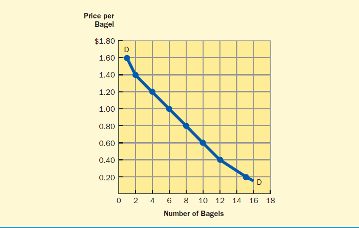
The downward-sloping demand curve illustrates the Law of Demand, showing that Zach demands fewer bagels at higher prices and more bagels at lower prices.
Supply: The Seller's Side
Economists refer to supply as a seller's plan to make a good or service available in the market. Like demand, supply depends on the product's price and any nonprice factors that influence the seller, such as the cost of producing the product and the seller's expectation of future market conditions.
Supply, Defined Economists define supply as the different amounts of a good or service that a seller would make available for sale at different prices in a given time period, holding constant all nonprice factors that affect the seller's plans for the product. In other words, supply indicates how many hot fudge sundaes, haircuts, tires, or any other product a supplier would be willing to sell at different prices during a week, a month, or a year, with all nonprice factors unchanged. As with demand, we hold all nonprice factors affecting supply constant to highlight the relationship between a product's price and the quantity of the product supplied.
Supply
The different amounts of a product that a seller would offer for sale at different prices in a defined time period when all nonprice factors are held constant.
We can illustrate the relationship between the amount of a product a seller would make available for sale and the product's price in a supply schedule (or table). Table 3.2 shows the number of bagels of a particular size and quality that City Bakery is willing to sell each week at various prices. Observe the direct relationship between price and the quantity supplied. At a low price, the bakery would offer no or few bagels for sale, but it is willing to offer more bagels for sale as the price increases. If we were to choose to illustrate the supply of another good or service as an example, the same relationship would appear: The quantity supplied would increase as the price increased, and the quantity supplied would decrease as the price decreased.
Supply Schedule
A list of the amounts of a product that a seller would offer for sale at different prices in a defined time period when all nonprice factors are held constant.
TABLE 3.2 City Bakery's Weekly Supply of Bagels
The Law of Supply is illustrated in this supply schedule, which shows that more bagels are supplied at higher prices.
| Price per Bagel | Quantity Supplied per Week |
| $0.20 | 0 |
| 0.40 | 50 |
| 0.60 | 200 |
| 0.80 | 350 |
| 1.00 | 500 |
| 1.20 | 650 |
| 1.40 | 750 |
| 1.60 | 800 |
The Law of Supply The direct relationship between price and quantity supplied illustrates the Law of Supply. This law states that, holding nonprice factors constant, the quantity of a good or service that a supplier is willing to offer on the market relates directly to price. Why does the bakery react this way? Seller behavior and the Law of Supply are based on a seller's ability to cover costs and earn a profit. At very low prices, a seller may not be able to cover costs and would likely not be interested in supplying the product. But as the price increased, a supplier could cover costs and perhaps earn a small profit. If a seller produced many products (as does City Bakery), it might produce some of the product for a small profit but concentrate on producing other items that yield more favorable returns. At higher prices, a seller would want to further increase the quantity supplied as it could cover additional costs from producing more and make greater profits.2 The bakery, for example, might be willing to decrease its production of birthday cakes, danishes, eclairs, and other products in order to increase its production of bagels if the price and profit on bagels were extremely high.
Law of Supply
There is a direct relationship between the price of a product and the quantity supplied.
We can easily understand the Law of Supply in relationship to our own labor that we supply in labor markets. Take campus tutoring as an example. If you were offered a job in the Economics Tutoring Center for $3 an hour, how many hours a week would you be willing to work? How much would you be willing to work if the wage were $10 an hour? $20 an hour?
Graphing Supply Economists usually present supply, like demand, graphically, with price measured on the vertical axis and the quantity supplied measured on the horizontal axis. Each price–quantity combination from Table 3.2 appears in Figure 3.2, and a supply curve is drawn by connecting those points. Note that a supply curve slopes upward, showing that higher prices correlate with larger quantities supplied. Recall that the Law of Supply indicates a direct relationship between price and quantity supplied. Because direct relationships appear in graphs as upward-sloping lines, we can generalize that supply curves slope upward to reflect that direct relationship.
Supply Curve
A line on a graph that illustrates a supply schedule; it slopes upward because of the direct relationship between price and quantity supplied.
FIGURE 3.2 City Bakery's Weekly Supply of Bagels

The upward-sloping supply curve illustrates the Law of Supply, showing that more is supplied at higher prices and less is supplied at lower prices.
You might be amazed at how often we are affected by the Laws of Demand and Supply. Application 3.1, “The Laws of Demand and Supply,” focuses on gasoline and organic milk and gives some situations where price had an important impact on the decisions and behaviors of buyers or sellers.
MARKET DEMAND, MARKET SUPPLY, AND PRICE SETTING
Market Demand and Market Supply
When buyers and sellers come together to exchange goods or services, they form markets. A market can arise anywhere—a store, eBay, used-car lot, stock exchange, or vending machine, for example. Once we speak of multiple buyers and sellers, we move from individual demand and supply to market demand and market supply. Market demand and market supply represent the sum of all individual quantities demanded and supplied of a product at each price in a market. For example, the market demand for an Academy Award-winning motion picture sums up all the individual demands to see the film. When we discuss markets we are concerned with the sum of all buyers' and sellers' actions—rather than individual demand and supply decisions.
Market
A place or situation in which the buyers and sellers of a product interact for the purpose of exchange.
Market Demand and Market Supply
The demand of all buyers and supply of all sellers in a market for a good or service; found by adding together all individual demand or supply schedules.
Markets and Price Setting
Markets perform the critical function of price setting as buyers and sellers interact and make economic choices. To see how markets operate to set prices, let's return to the bagel example, where we analyzed Zach's individual demand and City Bakery's individual supply of fresh-baked bagels.
APPLICATION 3.1
 THE LAWS OF DEMAND AND SUPPLY
Law of Demand
Gasoline Gasoline prices often rise rapidly on the rumor of some event that will affect the supply of oil coming to refineries. And, if reality is attached to the rumor, there can be an extended period of high prices. For example, threats by Iran to close the Strait of Hormuz, through which 20 percent of the world's oil flows, brought an immediate response of higher prices, but the actual closing would have a greater, far-reaching, longer impact.
And when those prices rise, consumer frustration usually leads to altered behaviors in purchasing gasoline. Some people might drive a few miles to wholesale stores for discounted gas; some who live along state borders have driven to the state with the lower gasoline tax rate; and some spend a lot of time waiting in line at the station with the cheapest price. People become more careful and consider the necessity of a trip to the mall or visits with friends and relatives, often forgoing them. One unfortunate result is the increase in thefts when prices go up, especially by drivers pulling away from a gas pump without paying.
If the price increase is sustained, more radical behavior changes occur. People begin to car pool and use public transportation. They may sell their gas guzzlers and search for and purchase vehicles with higher gas mileage. Sometimes people move to a neighborhood or suburb closer to work and the sports, cultural, and health amenities they frequent.
What drives these reactions to higher gas prices? We all have limited incomes, and paying more for gas means having less for other things like tuition, mortgage payments, and fresh produce. But, unlike many other consumer needs, the alternatives to putting gas in the tank aren't easy. It is not like switching to chicken when the price of beef increases. Can you just put a tank of corn-based ethanol in your vehicle or switch your internal combustion engine to an electric motor? Can you just zip over to the car dealership and switch out your car for a hybrid?
Law of Supply
Organic Milk In the “olden” days, people went to the store and bought milk—milk was milk. Dairy farmers had few alternatives: they milked their cows and sent their product to the market. Today, we have choices about milk: whole, skim, 1 percent, 2 percent, and even chocolate. While these don't have a direct influence on dairy farmers, the latest opportunity for choice in milk selection—organic milk—certainly does.
Organic milk is a major product in the trend toward buying organic foods. To be labeled as organic milk, a set of federal standards must be met. These include guidelines about feed, soil, outdoor access for cows, processing operations, as well as a ban on antibiotics and growth hormones.
While the route to become an organic milk producer cannot be put in place overnight because time is needed to ensure that operations and herds meet the standards set to receive the organic label, dairy farmers now have an alternative to producing “regular” milk. This means that as the price of organic milk rises, farmers have an incentive to switch production from nonorganic to organic.
And, the price of organic milk is certainly higher than nonorganic milk. A visit to the Schnuck's supermarket in St. Louis in October 2012 revealed that a gallon of nonorganic 2 percent milk was $3.38. A gallon of organic 2 percent milk was $5.99.
There is evidence that the rise in price in organic milk is increasing the quantity supplied. A few years ago, organic milk could be found only in specialty health-food type stores. Today, supermarkets not only devote much shelf space to organic milk, but like the St. Louis grocery store, typically carry several labels or brands.
Table 3.3 shows market demand and market supply schedules for fresh-baked bagels. We can find the market demand for bagels each week by adding together the number of bagels that Zach and all other tbuyers in this market would purchase at each price. Similarly, we can find market supply by adding together the quantity of bagels that City Bakery and all other sellers in this market would make available at each price. In the analysis of this market and those that follow, we assume that both buyers and sellers compete strongly with one another. No buyer or seller exerts any unusual or undue influence, and no price-controlling government regulation occurs.3
TABLE 3.3 Weekly Market Demand and Supply of Fresh-Baked Bagels
Market demand and market supply illustrate the different amounts of a product that all buyers in a market would demand and all sellers in a market would supply at various prices.
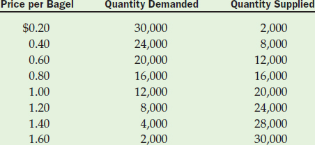
In the market shown in Table 3.3, the price for a fresh-baked bagel ranges from $0.20 through $1.60. What would happen in this market if the price were $0.20 per bagel? At $0.20, buyers would demand 30,000 bagels, and sellers would offer only 2,000 for sale. Thus, at a price of $0.20 the quantity supplied would fall short of the quantity demanded by 28,000 bagels (30,000 quantity demanded − 2,000 quantity supplied): The market would experience a shortage of 28,000 bagels. In response to this shortage, sellers who observed the number of buyers left unsatisfied in the market would raise the price and increase the quantity they would offer on the market (because of the Law of Supply). Once the price rose, the quantity demanded would fall (because of the Law of Demand), and the bagel shortage would shrink.
Shortage
Occurs in a market when the quantity demanded is greater than the quantity supplied, or when the product's price is below the equilibrium price.
So, then, what would happen if the price were $0.40 per bagel? At $0.40, buyers would demand 24,000 bagels and suppliers would offer 8,000 bagels. The market would again experience a shortage, but of only 16,000 bagels (24,000 quantity demanded − 8,000 quantity supplied). Sellers would react to the shortage by raising prices above $0.40. As price increased, suppliers would offer more bagels and buyers would demand fewer bagels: The shortage would again shrink.
What would happen if sellers charged $1.60 per bagel? At $1.60, consumers would want to buy only 2,000 bagels, but sellers would offer 30,000 bagels for sale. The quantity supplied would exceed the quantity demanded by 28,000 bagels, or there would be a surplus of 28,000 bagels on the market. Sellers would react like any other seller with excess merchandise at a price consumers will not pay: They would lower their prices. As the price fell, the Law of Demand would go into operation, and some buyers who would not purchase bagels at $1.60 each would do so at the lower price. At the same time, because of the Law of Supply, the lower price would encourage suppliers to reduce the quantity supplied, and the surplus would diminish. If the price charged were $1.40, a surplus of 24,000 bagels would develop, sellers would again lower their price, and the surplus would again shrink.
Surplus
Occurs in a market when the quantity supplied exceeds the quantity demanded, or when the product's price is above the equilibrium price.
FIGURE 3.3 Weekly Market Demand and Supply of Fresh-Baked Bagels
The equilibrium price and quantity in a market occur at the intersection of the market demand and supply curves. At equilibrium, the quantity demanded in a market equals the quantity supplied.
Equilibrium Price and Equilibrium Quantity
The market in Table 3.3 appears to be moving automatically toward a price of $0.80, where the quantity demanded equals the quantity supplied at 16,000 bagels. If sellers charge $0.80 per bagel, no surpluses or shortages will arise and sellers will have no incentive to raise or lower price.
We call the price that sets buyers' plans equal to sellers' plans ($0.80) the equilibrium price. The quantity at which those plans are equal (16,000 bagels) is the equilibrium quantity. Thus, equilibrium price and equilibrium quantity are the price and quantity toward which a market will automatically move. At the equilibrium price, quantity demanded equals quantity supplied, and neither sellers nor buyers will want to change the price or the quantity. Economists often refer to the equilibrium price as the market clearing price because at this price the amount that buyers want exactly matches the amount that sellers offer, thereby clearing the market of the good or service.
Equilibrium Price and Equilibrium Quantity
The price and quantity where demand equals supply; price and quantity toward which a free market automatically moves.
Market Clearing Price
Equilibrium price; price at which the quantity demanded equals the quantity supplied.
If the price of a good or service is below its equilibrium level, a shortage will develop, and the price will be driven up toward equilibrium. If the price is above equilibrium, a surplus will develop, causing the price to fall toward equilibrium.
The bagel market shown in Table 3.3 is graphed in Figure 3.3. We draw the demand curve from the Price per Bagel and Quantity Demanded columns, and the supply curve from the Price per Bagel and Quantity Supplied columns. From the graph, we can easily see that the equilibrium price and quantity lie at the intersection of the supply and demand curves—in this case, at a price of $0.80 per bagel and a quantity of 16,000 bagels.
Shortages and surpluses can also be illustrated graphically. Figure 3.4a shows that at a price of $1.20 the quantity demanded is 8,000 bagels and the quantity supplied is 24,000 bagels, a surplus of 16,000 bagels. The difference between the demand and supply curves at $1.20 equals the amount of the surplus. Notice that as the price comes closer to the equilibrium level, the distance between the demand and supply curves narrows, and the surplus becomes smaller. Figure 3.4b measures the shortage of 8,000 bagels that would occur at a price of $0.60. Can you determine the shortage at a price of $0.20 per bagel?4
FIGURE 3.4 Measuring Surpluses and Shortages on Demand and Supply Curves

The surplus or shortage at a particular price is equal to the difference between the quantity demanded and the quantity supplied at that price.
Changes in Quantity Demanded and Quantity Supplied
When the price of bagels in Table 3.3 and Figure 3.3 changed, the amount that buyers would have purchased also changed. For example, as the price rose from $0.20 to $0.40, the quantity demanded by buyers fell from 30,000 to 24,000 bagels. When a change in a product's price causes a change in the amount that would be purchased, a change in quantity demanded occurs. Graphically, a change in quantity demanded appears as a movement along a demand curve from one price–quantity point to another, such as from the point representing $0.20 and 30,000 bagels to the point representing $0.40 and 24,000 bagels on the demand curve in Figure 3.3.
Change in Quantity Demanded and Quantity Supplied
A change in the amount of a product demanded or supplied that is caused by a change in its price; represented by a movement along a demand or supply curve from one price–quantity point to another.
Likewise, the amount of bagels that the sellers in Table 3.3 and Figure 3.3 were prepared to sell changed as the price changed. As the price fell from $1.60 to $1.40, the quantity supplied fell from 30,000 to 28,000. When a change in a product's price causes a change in the amount of the product that a seller would supply, a change in quantity supplied occurs. A change in quantity supplied appears as a movement along a supply curve from one price–quantity point to another, such as from the point representing $1.60 and 30,000 bagels to the point representing $1.40 and 28,000 bagels on the supply curve in Figure 3.3. In the next section, we emphasize the difference between such changes in quantity demanded or supplied and changes in demand or supply.
CHANGES IN DEMAND AND SUPPLY
When we introduced demand and supply, we emphasized that the buyers and sellers of a product respond both to the product's price and to nonprice considerations. Then, as we developed demand and supply schedules and curves, we held nonprice factors constant in order to focus on buyer and seller behavior in response to a price change. For example, when we derived Zach's demand for bagels, only the price of bagels was allowed to change. All nonprice factors, such as Zach's income, the popularity of bagels, and the degree of substitutability between bagels and other foods were held constant.
Now it is time to no longer hold nonprice factors constant and to examine how nonprice factors influence buyer and seller behaviors—and ultimately how they influence market equilibrium.
Changes in Demand
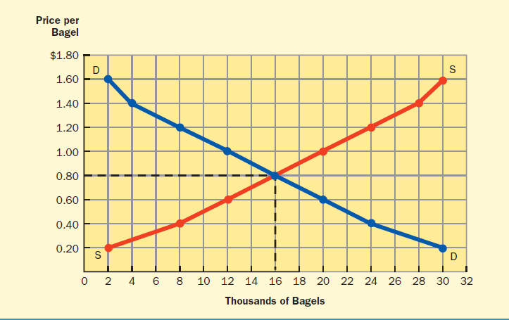
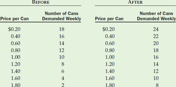
A change in one or more nonprice factors influencing the demand for a product causes a change in demand for the product. Changes in nonprice factors cause demand schedules and curves to change as buyers develop new sets of plans. Someone's weekly demand for, say, a particular brand of cola could change because of a change in a nonprice factor influencing that demand. For example, suppose that Gwen, who has a demand for a particular cola, gets a raise. She might respond to the raise by buying more cola. We can illustrate this increase in Gwen's demand in Table 3.4, which shows Gwen's demand for the cola before and after a change in her income. Notice how the number of cans that Gwen demands in a week increases at each price. For example, at $1.00 a can the amount increases from 10 to 16.
Change in Demand
A change in the demand schedule and curve for a product caused by a change in a nonprice factor influencing the product's demand; the demand curve shifts to the right or left.
TABLE 3.4 Gwen's Weekly Demand Schedule for 12-Ounce Cans of Cola before and after an Increase in Income
A change in a nonprice factor causes a change in the amount of an item demanded at each price. After an increase in Gwen's income, the number of cans of a particular cola she demands each week increases at every price.
Nonprice Factors That Influence Demand To help us see the key difference between price and nonprice factors, we can categorize major nonprice factors that influence demand.
Nonprice Factors Influencing Demand
Nonprice factors, such as income, taste, and expectations, that help to determine the demand for a product.
- Taste, fashion, and popularity. The demand for “in” items typically increases; and when an item is “out,” demand decreases. The recent focus on cupcakes, even fashioned as wedding cakes, has certainly shifted their demand to the right. A good, catchy advertising campaign that makes a product popular can increase demand.
- Buyers' incomes. Changes in buyer income can encourage people to buy more or less of an item. We label goods as normal goods when income changes relate directly to changes in demand: income increases generally lead to an increase in the demand for new cars. Goods are labeled as inferior goods when income changes relate inversely to changes in demand: income increases generally lead to a decrease in the demand for used cars. While these categories can be subjective, some goods are easy to identify as normal or inferior. How would you label ramen noodles, pro football game tickets, costume jewelry, fine watches, and vacation stays at a Marriott Resort or a Motel 6?
Normal Good (or Service)
Income changes relate directly to the demand for the good or service.Inferior Good (or Service)
Income changes relate inversely to the demand for the good or service. - Buyers' expectations concerning future income, prices, or availabilities. What people anticipate for the future affects behavior in the present. For example, if people think the price of gasoline will escalate in the coming weeks, they will fill their gas tanks as soon as possible and increase the current demand. What happens in local stores when a snow storm is anticipated and news reports focus on a shortage of ice melt?
- Prices of goods related as substitutes and complements. Buyers' demand for a product can change when the price of an item they regard as a substitute or complement for that product changes. For example, people might buy more peanut butter to make sandwiches when the prices of cheese or processed turkey slices (substitutes for peanut butter) go up. And, people might buy and send fewer holiday cards when the price of stamps (a complement to cards) increases.
- Number of buyers in the market. As the number of buyers in a market increases or decreases, so does demand. With people moving into newly renovated lofts in city neighborhoods, local restaurants and grocery stores have more customers. The reverse holds when residents begin to abandon a neighborhood.
Increases and Decreases in Demand We can label a change in demand as either an increase in demand or a decrease in demand. An increase in demand means that buyers want to purchase more of a product at every price because one or more nonprice factors have changed. Graphically, an increase in demand causes the demand curve for a good or service to shift to the right.
Increase in Demand
A change in a nonprice influence on demand causes more of a product to be demanded at each price; the demand curve shifts to the right.
Such a shift is shown in Figure 3.5a, which illustrates Gwen's demand schedules for cola in Table 3.4. Curve D1 shows Gwen's original demand for cola before her change in income. When Gwen's income increases, and she wants to purchase more cola at each price, her demand schedule changes. When this new schedule is graphed in Figure 3.5a, the demand curve shifts to the right, to D2. Observe on the graph that at $0.80 she is now willing to buy 18 rather than 12 cans, and at $1.20 she is now willing to buy 14 rather than 8 cans. Clearly, she demands more at each price, or has experienced an increase in demand.
A decrease in demand means that buyers want to purchase less of a product at every price because of a change in a nonprice factor. Graphically, a decrease in demand causes the demand curve to shift to the left. For example, U.S. consumers frequently change their vehicle preferences. At one time the large SUV was the choice of families. But today households are turning toward hybrids and away from large gas-guzzling SUVs. Figure 3.5b shows a change in the demand for large SUVs as consumer tastes change. Where 225,000 were demanded at a sticker price of $34,000 before the change in taste, only 125,000 are demanded after large SUVs become less popular.
Decrease in Demand
A change in a nonprice influence on demand causes less of a product to be demanded at each price; the demand curve shifts to the left.
In summary, an increase in demand means that more of a product is demanded at each price and the demand curve shifts to the right. A decrease in demand means that less is demanded at each price and the demand curve shifts to the left.
Changes in Supply
Changes in nonprice factors that influence supply cause entire supply schedules and curves to change, or cause changes in supply. Changes in these nonprice factors cause the supply curve to shift either to the right (an increase in supply) or to the left (a decrease in supply).
Change in Supply
A change in the supply schedule and curve for a product caused by a change in a nonprice factor influencing the product's supply; the supply curve shifts to the right or left.
Nonprice Factors That Influence Supply Just as for demand, we can categorize nonprice factors that influence supply.
Nonprice Factors Influencing Supply
Nonprice factors, such as the cost of production and the number of sellers in the market, that help to determine the supply of a product.
- Cost of producing an item. When a seller experiences a change in the production costs of a good or service, more or less of that good can be made available at each price. Increases in production costs cause less to be made available. When the price of a barrel of crude oil (the basic material for refining gasoline) increases on the market, the supply of gasoline decreases. Decreases in production costs cause more to be made available. Technology has made it cheaper to produce many electronics on the market today.5
FIGURE 3.5 Increases and Decreases in Demand

An increase in Gwen's demand for a cola causes the demand curve to shift to the right from D1 to D2, indicating that she now demands more cans of the cola at each price. A decrease in the demand for large SUVs causes the demand curve to shift to the left from D1 to D2, indicating that fewer are demanded at each price.
FIGURE 3.6 Increases and Decreases in Supply

An increase in the supply of digital cameras causes the supply curve to shift to the right from S1 to S2, indicating that sellers offer more at each price. A decrease in the supply of health club memberships causes the supply curve to shift to the left from S1 to S2, indicating that fewer memberships are supplied at each price.
- Expectations about future market conditions. Just as with buyers, sellers can anticipate future conditions that affect their current behavior. When grocery managers anticipate that consumer incomes will fall, they may change their inventory and decrease their supply of fresh berries and imported cheeses while increasing their supply of boxed mac and cheese and canned tuna.
- Other items the seller does, or could, supply. If a seller finds a profitable alternative item to offer for sale, it could affect the supply of other items. If an online university finds that it can increase its enrollment, tuition revenue, and profit by offering more Spanish language courses, it might lessen the language classes it offers in Polish or Japanese.
- Number of sellers in the market. As competition increases and more sellers enter a market, the supply increases. When sellers leave a market, supply decreases. Take the coffee shop phenomenon. In towns and neighborhoods, more and more coffee shops keep opening, increasing the supply of places to enjoy lattes and conversation.
Increases and Decreases in Supply An increase in supply means that sellers want to offer more of a good or service for sale at each price and that the supply curve for the good or service shifts to the right. In Figure 3.6a, assume that S1 is the original supply curve indicating that sellers of digital cameras were willing to sell 50,000 at $150 each or 80,000 at $200 each. After an increase in supply, which causes the supply curve to shift to S2, sellers are willing to offer more cameras at each price: for example, 80,000 at $150 and 110,000 at $200. The increase in supply could have come from lower production costs, new production technology, or sellers trying to increase sales now for fear of a weakening market in the future.
Increase in Supply
A change in a nonprice influence on supply causes more of a product to be supplied at each price; the supply curve shifts to the right.
APPLICATION 3.2
THE RISE AND FALL OF LOW CARBS
At one time, diets that promised better health by lowering carbohydrates, or “carbs,” were the rage. Carbohydrates are a source of energy found in bread, pasta, sugar, and other foods. With these popular diets, carbs were a no-no. Around the country, college cafeterias, fast-food eateries, and homemakers were adjusting the way they cooked and served food.
As these diets became popular and people changed their eating habits, the demand for low-carb foods went up and the demand for high-carb foods fell. Sales of beef, pork, and other low-carb foods jumped, while the demand for baked goods, pastas, and other higher-carb foods tumbled.
While some producers were hurt by the increased demand for lower-carb foods, others saw an opportunity to earn more profit through bringing new products to the market. General Mills, Progresso, Betty Crocker, Kellogg, Kraft, and Hershey's, to name a few, introduced diet-conscious buyers to new low-carb meal-replacement bars, soups, baking mixes, cookies, and other food products.
But just as fads appear, they also disappear. As the enthusiasm for these low-carb diets faded, so did the demand for low-carb foods in grocery stores and restaurants. This drop in demand sent a strong signal to food producers: The expected profit from low-carb items would likely not appear. And just as quickly as they had raced to introduce new products to the market, they raced to pull them out. Frito-Lay pulled its low-carb Doritos, Tostitos, and Cheetos after only six months on the market, and both Kraft and Keebler stopped production of their low-carb cookies. And many other low-carb products ended up in closeout bins.
A decrease in supply means that sellers are willing to offer less of a product at each price because one or more nonprice factors have changed. Figure 3.6b shows the original supply curve for an area's health club memberships as S1, indicating that clubs were willing to sell 1,400 memberships at a price of $200 each. A decrease in supply, represented by a shift of the supply curve to S2, reveals that clubs are now willing to sell fewer memberships at each price, for example, only 800 at $200 each. Sellers could have decreased the supply because of increased wage, equipment, or liability insurance costs, or could have switched to the production of another item that is more profitable.
Decrease in Supply
A change in a nonprice influence on supply causes less of a product to be supplied at each price; the supply curve shifts to the left.
In summary, an increase in supply means that a larger quantity of a product is made available for sale at each price, causing the supply curve to shift to the right. A decrease in supply means that a smaller quantity is made available for sale at each price, causing the supply curve to shift to the left. Application 3.2, “The Rise and Fall of Low Carbs,” shows how nonprice factors influenced the demand and supply of some types of foods.
Changes in Quantity Demanded or Supplied and Changes in Demand or Supply: A Crucial Distinction
Be warned: We must maintain clear distinctions between changes in quantity demanded and quantity supplied, and changes in demand and supply. Although the terms are similar, they refer to completely different concepts.
Changes in quantity demanded and quantity supplied arise only from changes in a product's price. Quantity is a variable tied to price. We illustrate the responses to price changes by movements along fixed demand or supply curves from one price–quantity combination to another. For example, the movement along the demand curve in Figure 3.7a from $20 and 100 units to $10 and 150 units illustrates an increase in quantity demanded caused by a decrease in price. The movement along the supply curve in Figure 3.7b from $20 and 100 units to $10 and 50 units illustrates a decrease in quantity supplied caused by a decrease in price.
FIGURE 3.7 Changes in Quantity Demanded and Quantity Supplied versus Changes in Demand and Supply

Changes in quantity demanded or quantity supplied are shown by movements along a fixed demand or supply curve, but with changes in demand or supply, the entire curve shifts.
On the other hand, changes in demand and supply do not result from changes in a product's price. Rather, they result from changes in a nonprice determinant of demand or supply. Changes in demand or supply appear as shifts of the demand or supply curve to the right or left.
In Figure 3.7c, the demand curve shifts to the right from D1 to D2, or there is an increase in demand because of a change in a nonprice influence on that demand. For example, at a price of $20, the amount demanded increases from 100 to 150 units. These could be great deep-dish pizzas that people might now order more often because word of their great taste has gotten around.
The shift of the supply curve in Figure 3.7d from S1 to S2 illustrates a decrease in supply. Fewer items are supplied at $20 and every other price because of a change in a nonprice factor. Perhaps this is a decrease in the supply of deep-dish pizzas caused by a rise in the cost of cheese, a key ingredient.
You will find it easier to understand the behavior of buyers and sellers in markets, and how they react to various price and nonprice considerations, if you remember these distinctions.
CHANGES IN EQUILIBRIUM PRICE AND EQUILIBRIUM QUANTITY
We have seen that when nonprice factors affecting demand or supply change, demand or supply curves shift. Recall that the equilibrium price and quantity of a good or service appear at the intersection of its demand and supply curves. Therefore, whenever a product's demand or supply curve shifts, its equilibrium price and quantity change as well.
Can we analyze and predict how changes in buyer and seller behavior alter both the equilibrium price of a product and the quantity bought and sold? Yes, we can by using the following tools to order our thinking about such changes in market conditions. Let's consider separately how each change in demand and supply affects equilibrium price and quantity.
Effect of Increases and Decreases in Demand
Increase in Demand How does an increase in demand affect a product's equilibrium price and quantity? Consider an item that becomes a fad. Suppose that volleyball becomes the “in” sport, and that all over the country people are searching for volleyball nets to put in their yards and take to parks and beaches. Common sense would tell us that the volleyball net market might heat up with such an increase in demand, and price would rise. But even at this increased price, more nets would be sold. Let's examine the graphical analysis in Figure 3.8a to determine whether our common-sense analysis is correct.
S is the monthly market supply curve for volleyball nets, and D1 shows the monthly demand for volleyball nets before the sport becomes a fad. With supply curve S and demand curve D1, the equilibrium price is $40 per net, and the equilibrium quantity is 25,000 nets. As the game becomes really popular, the demand for volleyball nets increases, and the demand curve shifts to the right to D2. At the new equilibrium of S and D2, 35,000 nets are sold to buyers at a price of $80 each. Thus, an increase in the demand for a product causes both its equilibrium price and equilibrium quantity to increase.
Decrease in Demand How does a decrease in demand affect a product's equilibrium price and quantity? Consider the market for mid-sized rental cars in a location popular with tourists during the summer months. Assume that S in Figure 3.8b is the weekly supply curve for mid-sized rental cars in this location and that D1 is the weekly demand curve for these cars during the summer. With S and D1, the equilibrium price is $300 per week and the equilibrium quantity is 1,200 cars.
But during the winter, fewer tourists visit this location and the demand for rental cars decreases. Figure 3.8b shows such a shift of the demand curve to the left from D1 to D2. As a result of this decrease in demand, the equilibrium price falls to $150 and the equilibrium quantity falls to 800. Thus, a decrease in the demand for a product causes both its equilibrium price and equilibrium quantity to fall. Consider the passing of a recent fad, like a singer who loses popularity with the young teen crowd. What happened to the price and quantity sold of that singer's recordings as the singer became less popular?
FIGURE 3.8 Effect of Increases and Decreases in Demand

An increase in the demand for a product, such as volleyball nets, causes an increase in the product's equilibrium price and equilibrium quantity. A decrease in the demand for a product, such as rental cars, causes a decrease in the product's equilibrium price and equilibrium quantity.
Effect of Increases and Decreases in Supply
Increase in Supply What effect does an increase in supply have on the equilibrium price and quantity of a product? We might respond immediately that an increase in the product's supply means that the price will fall and the amount sold will increase. Let's test this response.
Over the years, several products, such as cell phones, have become much more plentiful because technology has made them cheaper to produce and, hence, to supply. Many new companies have also entered the market. In Figure 3.9a, S1 and D are the original supply and demand curves for cell phones. With this supply and demand, the equilibrium price is $100 a unit, and the equilibrium quantity is 2 million units. Later, as new technologies and new manufacturers impact the market, the supply curve shifts to S2. Following this increase in supply, the new equilibrium price is $60 per unit, and the equilibrium quantity is 6 million units. Thus, with an increase in supply, the equilibrium price falls and the equilibrium quantity increases.
Decrease in Supply What will happen to a product's equilibrium price and quantity if supply falls? Assume that a virus is infecting chickens, causing fewer eggs to be produced, so that the supply of eggs decreases, but the demand for eggs does not change. D and S1 in Figure 3.9b are the demand and supply curves for eggs before the available amounts are reduced. With D and S1, the equilibrium price is $1.40 per dozen, and the equilibrium quantity is 12 million dozens. Suppose now that fewer eggs come to the market, causing the supply curve to shift to the left to S2. With this decrease in supply, the new equilibrium price is $2.10 per dozen, and the equilibrium quantity is 10 million dozens. Thus, a decrease in supply leads to an increase in the equilibrium price and a decrease in the equilibrium quantity of a product.
FIGURE 3.9 Effect of Increases and Decreases in Supply
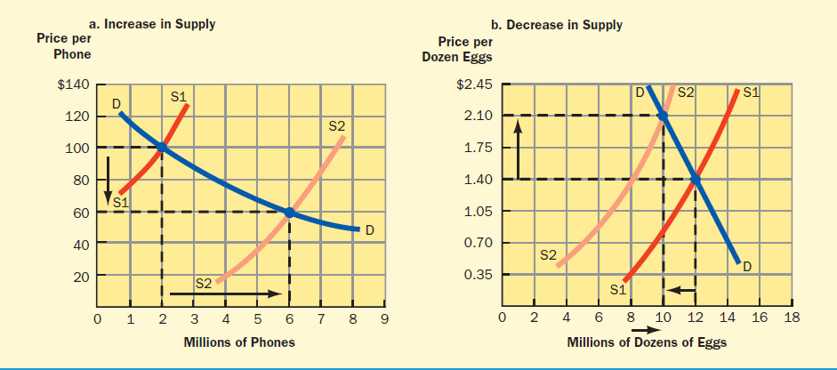
An increase in the supply of a product, such as cell phones, causes a decrease in the product's equilibrium price and an increase in its equilibrium quantity. A decrease in the supply of a product, such as eggs, causes an increase in the product's equilibrium price and a decrease in its equilibrium quantity.
Test Your Understanding, “Changes in Demand and Supply,” lets you evaluate your skill at analyzing the factors causing demand and supply curves to shift and the effects of those shifts on equilibrium price and quantity.
Effect of Changes in Both Demand and Supply
In each of the preceding examples, we held constant one side of the market—either demand or supply—to examine the effects of changes in nonprice factors. In reality, both demand and supply might change simultaneously. For example, both the demand and supply of volleyball nets or cell phones might increase at the same time. Although such simultaneous changes are not illustrated here, your graphing skills should enable you to arrive at some conclusions about them.6
TEST YOUR UNDERSTANDING
 CHANGES IN DEMAND AND SUPPLY
Complete the table by determining which of the following each example represents.
- An increase in demand
- A decrease in demand
- An increase in supply
- A decrease in supply
- No change in either demand or supply

Answers can be found at the back of the book.
LIMITING PRICE MOVEMENTS
Up to this point, we have dealt with free-market conditions, where buyers and sellers interact independently without any kind of outside intervention. But sometimes governments step into certain markets and interfere with free pricing by setting upper or lower limits on prices. State governments, for example, have limited prices on utilities, home mortgage interest rates, and interest rates on credit cards. The federal government has propped up prices for other goods and services, such as labor (with the minimum wage law) and some farm products. We can use supply and demand analysis to explain how this type of government intervention affects market conditions.
Price Ceilings
Legally imposed upper price limits, called price ceilings, keep prices from rising above certain levels. Price ceilings have been placed on gas and electricity in some states, rental apartments, and the interest rates people pay to borrow money. If the market goes to equilibrium at a price below the government-established upper legal limit, or ceiling, the ceiling will have no impact on buyers and sellers: The ceiling will not take effect. But if the market tries to go to an equilibrium price above its upper legal limit, the price ceiling will take effect and a shortage will occur.
Price Ceiling (Upper Price Limit)
A government-set maximum price that can be charged for a good or service; if the equilibrium price is above the price ceiling, a shortage will develop.
For example, suppose that a state law sets the maximum interest rate on student loans at 12 percent. Such laws that set maximum interest rates are called usury laws. Figure 3.10a gives the demand for and the supply of loans when the equilibrium interest rate is lower than the ceiling rate—so the ceiling has no impact. Here borrowers' and lenders' plans balance at an interest rate of 10 percent, and $10 million is loaned each month. Do you see that, because the government-imposed ceiling on interest rates lies above the equilibrium rate, the usury law is irrelevant in this case?
Usury Laws
Laws setting maximum interest rates that can be charged for certain types of loans.
Suppose, however, that more students want to borrow money, causing the demand curve to shift to the right. This new situation appears in Figure 3.10b. If the market were free to go to equilibrium after this increase in demand, the new interest rate would be 14 percent. However, the upper legal limit is 12 percent, so lenders may charge no more. Rather than increasing from 10 to 14 percent, the interest rate can rise only to the legal limit of 12 percent. At the 12 percent rate, borrowers would like to have $16 million in loans, but lenders would provide only $12 million in funds. At the 12 percent usury limit, there would be a $4 million shortage of funds for borrowing. Thus, when the free-market equilibrium price is above the ceiling, a shortage develops.
Price Floors
Legally imposed lower price limits, called price floors, prevent prices from falling below certain levels. Examples of price floors include the minimum wage law, which sets the minimum hourly payment that many workers can earn, and some government-guaranteed agricultural prices, which ensure that farmers will receive at least a set minimum price on particular crops. As long as the equilibrium price of a good or service is above its price floor, the free market will not be affected by the limit. However, if the equilibrium price of a good or service falls below the floor, buyers will be forced to pay the government-set price. Because this legally imposed price is higher than the price the free market would have permitted, sellers offer more than buyers want to buy at the set price, and surpluses develop.
Price Floor (Lower Price Limit)
A government-set minimum price that can be charged for a good or service; if the equilibrium price is below the price floor, a surplus will develop.
Consider the effect of the minimum wage law as an example. Suppose that the minimum wage is set at $8 per hour. If the supply and demand for a certain type of labor are as shown in Figure 3.11a, the minimum wage will have no impact on the market. The equilibrium wage of $9 per hour is greater than the minimum wage, and the number of available workers equals the number demanded.
FIGURE 3.10 Effect of a Price Ceiling on a Market
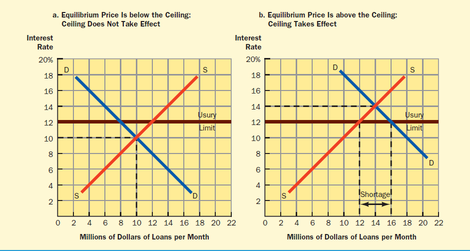
When the equilibrium price for a product is below its legal upper limit, the price ceiling has no effect on the market. When the equilibrium price is above its legal upper limit, the price ceiling takes effect and a shortage develops.
Now suppose that the government raises the minimum wage from $8 to $10 per hour, but that neither the supply nor demand for labor changes in this market. Because the equilibrium wage rate is $9, or less than the minimum wage, the $10 minimum wage will take effect. That is, businesses buying this type of labor must pay $10 per hour rather than $9. Figure 3.11b shows the market condition with the new minimum wage rate. At $10 per hour the number of workers demanded falls to 1,000, and the number of willing and able workers rises to 1,200. The price floor has created a surplus of 200 people who cannot obtain a job in this market. Thus, when the free-market equilibrium price is below the government-imposed floor, a surplus develops.
In summary, price ceilings, when they take effect, keep prices lower than they would otherwise be and result in shortages. Price floors, when they take effect, keep prices higher than they would otherwise be and result in surpluses. Price ceilings and price floors benefit some groups and hurt others. Application 3.3, “Is Rent Control a Good Thing or a Bad Thing?,” explores some issues around the setting of ceilings on rents for apartments in New York City. Hopefully, the application will help you recognize why it is difficult to arrive at a clear answer to questions like who gains and who loses from rent control.
FIGURE 3.11 Effect of a Price Floor on a Market

When the equilibrium price for a resource or a product is above its legal lower limit, the price floor has no effect on the market. When the equilibrium price is below its floor, the floor takes effect and a surplus develops.
Up for Debate, “Is It a Mistake to Raise the Minimum Wage?” applies this same question to labor markets. Who gains and who loses from an increase in the minimum wage?
We should note that government can also affect markets by influencing the supply side of the market. For example, local governments can limit the number of trash haulers in an area and the Food and Drug Administration controls the flow of new medications onto the market.
PRICE ELASTICITY OF DEMAND AND SUPPLY
One message in this chapter should be clear: The quantity of a good or service that consumers demand relates inversely to its price, and the quantity of a good or service that sellers supply relates directly to its price. But there is another piece of the buyer and seller puzzle. How much will quantities demanded and supplied change as buyers and sellers respond to a particular price change? If a bike shop offered a huge sale—say, 50 percent off—on its finest touring bicycles, would people line up around the block to buy top-of-the-line bikes for $2,000 (half off of the usual retail price of $4,000)? Would they more likely show up for a store's 50 percent sale on designer purses? When the price of an item—say peanut butter—increases, do consumers respond weakly, demanding just a little less of the item, or strongly, demanding much less? What about their response when the price of steak or fine wine increases?
APPLICATION 3.3
IS RENT CONTROL A GOOD THING OR A BAD THING?
Want to start an argument in New York City? Just bring up the subject of rent control. Likely, if there are two people within earshot, one will think it's wonderful and the other will think that, short of selling the Yankees, it is the best way to destroy the city. And what can begin as a civil discussion on the topic may well end as an intense battle of words.
Rent control was instituted in New York City in 1943 to help keep local residents from losing their apartments to better-paid transient wartime workers who could afford higher rents. Almost 70 years later, many of the city's rental units are still subject to some type of price control. In Manhattan alone, there are 16,000 remaining rent-controlled units.
Part of the argument over rent control comes from the stories about what people pay in rent-controlled versus uncontrolled units. It was reported that Faye Dunaway had a $1,000 a month rent-stabilized unit for decades on the Upper East Side. Then there is the 80-year old man who has lived for 50 years in a four-bedroom in Greenwich Village for $331.76 a month, where the average two-bedroom rents for over $4,700 a month and a town house down the block was for sale at $5 million. Or there is the woman who lived for over 30 years in a rent-controlled one-bedroom suite in a hotel overlooking Central Park for $8 a day while hotel guests paid up to $1,600 a day. And, compare this with the student working as a doorman, who along with two of his friends, paid $1,200 a month in an apartment so small that one of them slept on the floor.
One of the arguments against rent control is that the rents are simply too low. One landlord complained that people in his neighborhood pay more to park than they pay to rent. Landlords often say that it is difficult to survive as their costs rise. Another argument is that rent control has nothing to do with need. Many well-to-do people who can comfortably pay more for their living accommodations live in rent-controlled apartments, keeping poorer families out of low-rent units. Sometimes a lone elderly person lives in a spacious three-bedroom apartment because moving to a smaller non-rent-controlled unit would be more costly. And sometimes families stay in increasingly dangerous neighborhoods because they don't want to pay more for housing. Also, there are the stories about black markets for rent-controlled apartments: “Let me sign a year's sublease and I'II give you $5,000 in cash under the table.”
But there are arguments on the other side of the debate. There are renters—like the man on disability who spends $400 of his monthly $600 check on rent—who might be living on the street were it not for the controlled rate. Recent studies of city data point out the large number of people in rent-controlled and rent-stabilized units who are making less than $15,000 a year. Also, while rent controls can be blamed for reducing people's mobility, they can also be credited for providing people with the stability that comes from being able to remain in one location, raise their families, and develop a network of friends over an extended period of time.
So, is rent control a good thing or a bad thing? Probably the safest answer is “it depends on who you talk to.”
Based on: “New York City Tenants, Landlords Keep Rent-Control Debate Raging,” Newsday, Knight Ridder Tribune Business News, June 18, 2003, p. 1; Laurie Cohen, “Some Rich and Famous in New York City Bask in Shelter of Rent Law,” The Wall Street Journal, March 21, 1994, pp. A1, A8; Nancy Keates, “Only in New York: Luxury at $8 a Day,” The Wall Street Journal (Eastern Edition), January 23, 1998, p. 1; Eileen Pollock, “Curse of Rent Control,” The New York Times, June 14, 2000; Daniel Rose, “The Theology of Rent Control: History of Low Income Housing,” Vital Speeches of the Day, August 15, 2003, p. 670; Ginia Bellafante, “Rent-Regulation Wars Are Only a Sideshow,” The New York Times, March 11, 2012, p. 22; Elizabeth A. Harris, “A Piece of the Manhattan Dream, Only $331.76 a Month,” The New York Times, January 24, 2012, pp. A18–19.
We can ask similar questions about sellers. Would automobile manufacturers respond weakly or strongly if the price of luxury cars dropped by 10 percent? How much corn would farmers plant next year if the price of corn rose 50 percent this year? How would computer hardware and software companies respond to a decrease in the price of their products?
Price elasticity measures the strength of buyers' or sellers' responses to a price change. If buyers or sellers respond strongly to a price change, we say that their demand or supply is price elastic. More specifically, demand or supply is considered to be price elastic when a given percentage change in price (say 5 percent) results in a larger percentage change in quantity demanded or supplied (say 6 percent or 10 percent). If buyers or sellers are less sensitive to a price change—that is, if their response is weak—we say that their demand or supply is price inelastic. Again, more specifically, demand or supply would be price inelastic if a given percentage change in price (say 8 percent) resulted in a smaller percentage change in quantity demanded or supplied (say 7 percent or 3 percent). The mechanics of calculating elasticities of demand and supply are explained in the appendix to this chapter.
Price Elasticity
A measure of the strength of buyers' or sellers' responses to a price change.
Price Elastic
A strong response to a price change; occurs when the percentage change in the quantity demanded or supplied is greater than the percentage change in price.
Price Inelastic
A weak response to a price change; occurs when the percentage change in the quantity demanded or supplied is less than the percentage change in price.
UP FOR DEBATE
 IS IT A MISTAKE TO RAISE THE MINIMUM WAGE?
Issue In 2007 Congress passed a law with phased increases in the minimum wage. The minimum wage would be raised from $5.15 to $5.85 per hour in July 2007, to $6.55 per hour in July 2008, and to $7.25 per hour in July 2009. Congress has raised the minimum wage several times since it was enacted in the 1930s. Clearly, any worker who takes home more money because the minimum wage has gone up is a winner. But some people think that raising the minimum wage is a mistake because some businesses, especially small ones, lose out when such mandated increases take effect. Is raising the minimum wage a mistake?
Yes It is a bad idea to raise the minimum wage. The higher wage may help workers who will now take home more income, but it also raises the cost of doing business for a worker's employer. These increased costs may force some small or financially strapped businesses to re-think their workforce needs and hire fewer workers in the future—or even lay workers off now. An increase in the minimum wage might be enough to push an employer to finally buy the machine that will, once and for all, replace workers, or to move its production operations to China, India, or some other country. And if a business cannot absorb the increased costs, it may be forced to close. What good does it do workers to be promised an increase in wages, only to lose their jobs as a result of that increase?
Also, if the new minimum wage falls above the equilibrium wage in a market, it will lead to an increase in the number of available workers at the very time that businesses are cutting back the number of workers demanded. Some people who would have had jobs at the lower equilibrium wage will now find themselves unable to obtain work. This may be a particular problem for college students looking for summer employment.
No It is not a mistake to raise the minimum wage for several reasons. For one, a scan of job advertisements shows that many people, such as those working in fast-food restaurants and college students seeking summer jobs, are already earning more than the minimum wage. To say these people would have greater difficulty finding or keeping work may overstate the problem created by an increase in the minimum wage.
But perhaps the strongest argument for raising the minimum wage is the inability to subsist on this wage. A person working eight hours a day, five days a week, fifty weeks a year at the minimum wage of $7.25 per hour would earn $14,500 for the year. By comparison, the official poverty-guidelines income in 2011 (when the minimum wage was $7.25) was $14,710 for the average two-person household. This reality is important for the minimum wage earner who is the only, or primary, source of income for a family. Not all minimum wage workers are high school or college students working part-time while living in a higher income household.
Source: The 2011 poverty level is from U.S. Department of Health and Human Services, “The 2011 HHS Poverty Guidelines,” http://aspe.hhs.gov/poverty/11poverty.shtml.
Price Elasticity of Demand
Why do consumers respond strongly to some price changes and weakly to others? In other words, what determines whether demand will be relatively price elastic or inelastic?
Factors Affecting Price Elasticity of Demand Several categories of factors affect price elasticity of demand.
- Necessities versus luxury goods. Generally, people respond more strongly when the price of a luxury good changes than they do when the price of a necessity changes. You would expect a fairly strong response by buyers to a price change on dinners at an upscale restaurant or cruises to Alaska. However, when a product is absolutely essential, people do not change their purchases very much, even when a price rise is substantial. Regardless of how much emergency medical care costs, parents will still generally take their seriously ill children to the ER. Typically, consumers respond weakly to price changes on necessities like water, gasoline, electricity, and prescription drugs. It is a lot easier to cut back on vacation plans than antibiotics.
- Substitutes. The availability of acceptable substitutes influences consumer responses to product price changes. If buyers can switch to similar or alternative products when prices rise, they will respond more elastically to a price change. If movie theater ticket prices increase, you can go to a concert or rent a DVD instead. On the other hand, if prices increase for a good or service with no or few substitutes, buyers may have little choice but to pay the higher prices: a price-inelastic response. When the price of a required textbook increases, for example, students have little choice but to buy it.
- Proportion of income. The portion of income that a purchase requires influences buyer responses to price changes. A person with an average income will likely respond weakly to a 20 percent increase in the price of a birthday card but respond strongly to a 20 percent increase in college tuition. The greater the portion of income required for a good or service, the stronger the reaction will be to a price change for that good or service, or the more price elastic will be the response.
Price Elasticity of Demand and Total Revenue The seller of a product needs to know whether buyers will react strongly or weakly to a price change. Without this information, a seller may be surprised by the impact that a price change has on the total revenue received from selling the product. This important concept could cause tremendous problems for the local transit authority, a theater venue, a homebuilder, or any other seller that misgauges buyer reaction to a price change.
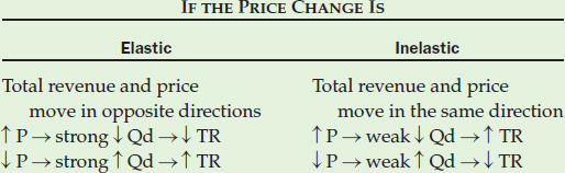
When customers react strongly, or there is an elastic response to a price change, total revenue moves in the opposite direction from the price change. If price is increased and consumers react strongly by demanding much less of a product, total revenue (price times quantity) will fall—the strong quantity response brings total revenue down with it. If price is decreased and consumers react strongly by demanding much more, total revenue will increase. If the owner of an Irish dance studio has 200 students who pay $50 a month for lessons, she receives $1,000 in revenue (200 × $50). If she raises the price to $60 a month and there is a strong student reaction causing a student drop to 150, her total revenue falls to $900 (150 × $60).
Elastic Price Change and Total Revenue
Total revenue moves in the opposite direction of a price change when consumers react strongly or elastically.
When buyers react weakly, or there is an inelastic response to a price change, total revenue moves in the same direction as the price change. If price is increased and consumers react weakly by demanding a little less, total revenue will rise with the price increase—the weak quantity response will not be enough to offset the effect of the price increase. If price is decreased and consumers react weakly by demanding just a little more, total revenue will decrease. Take the Irish dance studio with its 200 students paying $50 a month for lessons. If the owner increases the price to $60 and loses just 10 students, total revenue will increase to $1,140 (190 × $60).
Inelastic Price Change and Total Revenue
Total revenue moves in the same direction of a price change when consumers react weakly or inelastically.
Sellers need to know whether people will respond weakly or strongly to a price change. Think about your own college or university. When administrators ponder changing the price of tuition, they can make good decisions about their budgets and expenditures if they know whether students will respond elastically or inelastically to a given change. Imagine the surprise the finance office faces when they believe that students will not care about an increase they have made, but they do and react elastically.
TABLE 3.5 Price Elasticity of Demand and Total Revenue
Total revenue moves in the opposite direction of the price change when demand is elastic, and total revenue moves in the same direction as the price change when demand is inelastic.
APPLICATION 3.4
PEANUT BUTTER: A YUMMY STAPLE
Families, food banks, and other organizations devoted to hunger relief began to notice significant increases in the price of peanut butter in the fall of 2011. As the price of a ton of peanuts increased to about $1,200 a ton from $450 a ton a year earlier, companies that produce well-known brands of this staple announced increases of up to 40 percent. And, some folks jokingly said that children needed to hoard the Reese's Peanut Butter cups in their trick-or-treat bags.
Peanut butter is a necessity in the everyday life of many people. Not only do kids love the stuff—experts saying that the average kid will eat 1,500 PB&J sandwiches before high school—but it also provides an important and usually cheap source of protein. For some, peanut butter is the key ingredient in a meal; for others it is a snack.
Food banks rely on peanut butter for its popularity, long shelf life, and nutritional value. Moreover, the therapeutic food often used to treat malnourished children in poor countries, such as Haiti, is created from ground roasted peanuts.
The quick rise in the price of peanut butter in 2011 and 2012 is a classic example of the application of supply and demand. Nonprice factors drove changes in the market and price influenced the quantity demanded.
Clearly, the underlying problem of the rise in peanut butter prices was on the supply side. It began with a short crop in the summer of 2010 when a drought negatively affected the supply of good, usable peanut kernels. But the summer of 2011 was calamitous for peanut farmers. Record-breaking heat and drought in the two largest peanut growing states, Georgia and Texas, brought a small crop. Since the peanut plant flowers above ground but eventually grows downward into the soil, some plants were badly scorched by the sun and never developed while other plants produced a low yielding, poor quality crop. And, as the planting season approached, some farmers switched their fields to cotton or soybeans since the prices on these major crops were high.
As the supply of peanuts quite literally dried up, the price began to rise. And, now there was concern about how families and food banks and hunger relief groups would deal with the rising price of this nutritional commodity. Moreover, a recession with its high unemployment increased the dependence on this cheap source of food by struggling families and also increased the number of clients reaching out to food banks.
Some food banks said they needed to buy less peanut butter to deal with their own limited budgets and that they were receiving fewer donations of peanut butter. This resulted in a cut back on the amount of peanut butter they gave out. Further limitations to supply came from the smaller amount of peanut butter available through U.S. agricultural commodity programs for schools and nonprofits.
Price Elasticity of Supply
Price elasticity also applies to sellers. How much more will sellers be willing to supply at a higher price, and how much less at a lower price? If sellers respond strongly to price changes, we say that supply is price elastic. If they respond weakly to changes in price, we say that supply is price inelastic.
Factors Affecting Price Elasticity of Supply For most sellers, price elasticity of supply is primarily affected by time. The more time sellers have to react to a price change, the greater is the ability to change the quantity supplied, and the more elastic is the response. Suppose that a particular style of jeans becomes very popular and the increase in demand pushes up its price. Sellers of these jeans can initially supply only as many pairs as the inventory on hand allows. Thus, the immediate response to this increase in price is inelastic. But given more time, sellers can order more jeans and respond with a larger increase in the quantity supplied—a more elastic response. Given even more time, other sellers and manufacturers may see how popular this style has become and may offer many more for sale. The jeans supply becomes even more price elastic.
Application 3.4, “Peanut Butter: A Yummy Staple,” looks at how supply and demand played out in the market for peanut butter. Can you explain how the relationship between demand and supply influenced price? How have nonprice factors and the elasticities of both demand and supply played a role?
Summary
- Demand refers to a buyer's willingness and ability to purchase different amounts of a product at different prices in a given period of time when all nonprice factors are held constant. The relationship between a product's price and the quantity buyers plan to purchase at each price is typically shown in a demand schedule or graph called a demand curve, which slopes downward. Demand schedules and curves reflect an inverse relationship between price and quantity demanded, called the Law of Demand. The Law of Demand results from limited buyers' incomes and substitute products.
- A supply schedule shows the different amounts of a product that a seller would offer in the market at different prices in a given time period when all nonprice factors are held constant. Graphically, a supply schedule appears as an upward-sloping supply curve because of the Law of Supply, which states that there is a direct relationship between price and quantity supplied. The Law of Supply follows from sellers' efforts to cover costs and earn profits.
- The total amount of a product demanded by all buyers in a market at a particular price is market demand, and the total amount made available by all sellers at that price is market supply.
- The price that equalizes buyers' and sellers' plans, and toward which a market automatically moves, is called the equilibrium price. Equilibrium price is at the intersection of the product's market demand and supply curves. If the market price of a product is above its equilibrium price, a surplus of the product will appear on the market, and forces will bring the price down to its equilibrium level. If the market price of a product is below its equilibrium level, a shortage will result, and forces will bring the price up to its equilibrium level.
- Nonprice factors also influence buyers' and sellers' behaviors. Changes in these nonprice factors lead to shifts in demand and supply curves. An increase in demand or supply means that buyers are demanding or sellers are supplying more of a product at each price, and the demand or supply curve has shifted to the right. When less of a product is demanded or supplied at each price, demand or supply decreases, and the demand or supply curve shifts to the left. Because the equilibrium price and quantity of a product are shown by the intersection of its demand and supply curves, increases or decreases in demand and/or supply cause the product's equilibrium price and quantity to change.
- It is important to understand the difference between changes in demand and/or supply, shown by shifts in the demand and/or supply curves, and changes in quantity demanded and/or quantity supplied, shown by movements along existing demand and/or supply curves. Changes in price cause movements along a demand or supply curve from one price–quantity point to another, or cause changes in quantity demanded or quantity supplied. Changes in nonprice influences cause shifts of demand or supply curves, or cause changes in demand or supply.
- If government sets a price ceiling for a good or service, and the equilibrium price is above the ceiling, the ceiling price takes effect and a shortage develops. If government sets a price floor for a good or service, and the equilibrium price is below the floor, the floor takes effect and a surplus develops.
- Price elasticity measures buyers' and sellers' sensitivities to changes in the price of a product. Demand or supply is price elastic when the quantity demanded or supplied changes by a greater percentage than the percentage price change. Demand or supply is price inelastic when the quantity demanded or supplied changes by a smaller percentage than the percentage price change. Elasticity of demand is influenced by whether the product is a luxury or a necessity, the availability of substitutes, and the price of the product relative to the buyer's income. Time is the major determinant of a product's price elasticity of supply.
- When the response by buyers to a price change is inelastic, total revenue moves in the same direction as the price change. When the response by buyers to a price change is elastic, total revenue moves in the opposite direction of the price change.
- (From the appendix) Price elasticity of demand or supply is calculated by dividing the percentage change in quantity demanded or quantity supplied by the percentage change in price. If the resulting number is greater than 1, demand or supply is price elastic. If the resulting number is less than 1, demand or supply is price inelastic. And if the resulting number is exactly 1, demand or supply is unitary elastic.
Key Terms and Concepts
Demand
Demand schedule
Law of Demand
Demand curve
Supply
Supply schedule
Law of Supply
Supply curve
Market
Market demand and market supply
Shortage
Surplus
Equilibrium price and equilibrium quantity
Market clearing price
Change in quantity demanded and quantity supplied
Change in demand
Nonprice factors influencing demand
Normal good (or service)
Inferior good (or service)
Increase in demand
Decrease in demand
Change in supply
Nonprice factors influencing supply
Increase in supply
Decrease in supply
Price ceiling (upper price limit)
Usury laws
Price floor (lower price limit)
Price elasticity
Price elastic
Price inelastic
Elastic price change and total revenue
Inelastic price change and total revenue
From the appendix
Elasticity coefficient
Unitary price elastic
Review Questions
- Define the Law of Demand and Law of Supply. Draw a demand curve and a supply curve and explain how each curve illustrates the related law. Identify the factors underlying these laws.
- Surpluses and shortages are temporary conditions in freely operating markets. Explain what causes each and how these temporary conditions resolve themselves in free markets.
- Distinguish between a change in quantity demanded or quantity supplied, and a change in demand or supply. How would you represent each change graphically?
- Explain how each of the following would cause demand or supply to shift and how the equilibrium price and quantity for the good or service in question would change.
- A decrease in the number of builders in a housing market
- Expectations by automobile buyers that new, more efficient hybrids will be on the market next year
- An increase in the popularity of organic peanut butter
- A wage increase paid to a hospital's employees
- A cost-reducing innovation adopted by the producers of a mobile communication device
- The identification of a food as high in cholesterol
- A fall in income by buyers of fine antique jewelry
- Plot the following demand and supply schedules on the accompanying graph, and answer questions a through e.
- What is the equilibrium price and equilibrium quantity?
- How much of a shortage or surplus would occur at $2.50?
- How much of a shortage or surplus would occur at $7.50?
- What would happen if the government established a price floor of $8.75 on this item?
- What would happen if the government established a price ceiling of $8.75 on this item?

- What does price elasticity of demand and of supply measure? Identify factors that affect these price elasticities and give examples of each.
- (From the appendix) Calculate the price elasticity coefficient of demand or supply for each of the following. Identify whether the response is elastic, inelastic, or unitary elastic.
- The number of cans of a soft drink demanded increases by 30 percent after its price decreases by 40 percent.
- The number of available apartments increases by 8 percent following a 6 percent increase in rents.
- The number of Cobb salads demanded at a restaurant increases from 60 to 80 per week when the price falls from $10.00 to $9.00.
- At a price of $200, 10,000 gas grills were supplied each month. Since the price increased to $250, 14,000 are supplied each month.
- The number of movies rented each weekend falls from 500 to 400 following an increase in the rental charge from $2.00 to $2.40.
Discussion Questions
- People pay attention to political upheavals in foreign countries, local and national elections in the United States, and environmental and other developments around the world because such events can directly affect their lives. But the functioning of markets may go relatively unnoticed because market effects are usually less obvious or dramatic. How does the functioning of markets affect your everyday life? If prices were not set in markets, how else could they be determined? How would this affect your life?
- We placed great emphasis on the distinction between changes in quantity demanded and quantity supplied and changes in demand and supply. Why would an automobile dealership treat buyers' reactions to price changes differently than it would their reactions to changes in everything else that affects their purchasing decisions? Does that seller have any control over nonprice determinants of demand, such as buyer taste? How and why?
- Both real and perceived differences arise among the kinds of entertainment, food, and clothing that are popular among buyers in different age groups. Pick one product from each of these three categories that is popular with your age group and explain how its demand and equilibrium price would change if it were marketed to people older than you. How would the cost of this increased marketing affect its equilibrium price and quantity?
- Minimum wage laws keep many workers' hourly wages above what they would be in the absence of such laws. Do minimum wage laws help or hurt college students looking for summer work?
- If a government-imposed price ceiling or floor helps some people but hurts others, what factors do you think the government should consider before deciding on such a policy? (You might consider interest rate ceilings on credit cards and student loans, and price supports on milk in answering this question.)
- Give some examples of goods and services where a consumer's response to a price change might typically be elastic and where it might typically be inelastic. Explain why the response would be elastic or inelastic.
- How does price elasticity of demand determine whether a seller's revenue will increase or decrease following an increase in the price of its product? What impact might the cost of production have on a seller's decision to change its price?
Critical Thinking Case 3 
HOW DO SUPPLY AND DEMAND WORK IN HEALTH CARE?
Critical Thinking Skills
Identifying exceptions to a norm
Comparing applications of a principle in different settings
Economic Concepts
Supply and demand
Pricing
About a year ago, John decided that, with 160,000 miles on his 2004 Volvo, the time had come to buy a new car. He was successful in his job and wanted to update his look. Because John knew this would be expensive, he spent a good bit of time reading reports about different models, shopping online, and going from dealer to dealer. Finally, after three weeks of visits to showrooms, John found a car he really liked. Its price tag was $31,000. John wanted the car, but this didn't stop him from trying to talk the dealer down from the $31,000 sticker price because he had done enough research to know this was possible. After a few days of phone calls back and forth, John bought the car for $22,000 plus his 2004 Volvo in trade.
About three weeks later, John called a doctor after having severe knee pain following a fall. The doctor told him to come in for a checkup as soon as possible. After an exam and some tests, John's doctor recommended surgery. With John's agreement, the doctor scheduled all of the routine presurgery testing as well as the surgery at South City Hospital where he is on staff. There are other hospitals closer to John's home, but John didn't bother to ask about going to one of them. He also did not ask about the costs involved with the testing and surgery.
Shortly after arriving at the hospital, John was assigned to a room on the third floor. He was surprised to see how many beds on the floor were empty. After surgery and post-op recovery, John's doctor gave him two prescriptions, released him from the hospital, and set appointments for checkups and physical therapy. John collected his belongings, paid his co-payment for his health insurance, and hobbled out the door. On his way home, he filled and paid for his prescriptions. He didn't bother to ask the pharmacist if there were cheaper generic drugs he could use in place of his prescriptions. He was just happy to be on his way home.
Later in the month John totaled up the bills for his doctor's visits, hospital treatment, medications, and therapy. They came to $31 000.
Questions
- Contrary to conventional economics, physicians (the suppliers) typically decide the quantity and type of health care services their patients (the demanders) will purchase. What is it about medical services that usually allows the supplier to determine the demand?
- Suppose a person who knows nothing about auto maintenance takes a car in for its 30,000-mile checkup. The service manager reads off a list of repairs that need to be done. In your opinion, will this person act like John did on learning the doctor's diagnosis? Does the market for auto repairs behave like the market for medical care? Should it?
- Many people have a large part of their health care expenses paid by an insurance provider. Explain how this might lead patients to pay little attention to the price of their treatment. Other than insurance coverage, what other factors would cause a patient to pay little attention to the price of a treatment?
- Conventional economics suggests that a business with unsold, or surplus, merchandise will lower its price to attract buyers. Do you think that a physician would lower the price of a procedure or a hospital would lower its daily bed rate to attract patients?
CHAPTER 3 APPENDIX
MEASURING PRICE ELASTICITY
The degree to which demand or supply is price elastic or inelastic can be measured by calculating an elasticity coefficient from the formula:
Elasticity Coefficient
The absolute value of the percentage change in quantity demanded or supplied divided by the absolute value of the percentage change in price; greater or less than 1 when demand or supply is price elastic or inelastic, respectively.
![]()
where Q represents the quantity demanded or supplied of a product, and P represents the product's price. The vertical lines on each side of the numerator and denominator indicate that we are interested in the absolute values of the percentage changes in quantity and price. Absolute value focuses on the size of a change but not its direction. Whether the change in price or quantity is up or down, or has a plus or minus sign in front of it, is not important in calculating elasticity: All changes are treated as though they are preceded by a plus sign.1
When demand or supply is price elastic, a given percentage change in price leads to a greater percentage change in quantity demanded or quantity supplied. Using the formula, the elasticity coefficient is greater than 1. When demand or supply is price inelastic, a given percentage change in price leads to a smaller percentage change in quantity demanded or quantity supplied. Using the formula, the elasticity coefficient is less than 1.
If the quantity demanded of a particular shoe falls by 20 percent after its price rises by 10 percent, demand is price elastic because the percentage change in quantity demanded is greater than the percentage change in price. Specifically, when the elasticity coefficient is calculated,
![]()
the number is greater than 1, indicating that demand is price elastic. If the quantity demanded of the shoe decreases by 8 percent following a 10 percent price increase, demand is price inelastic because the percentage change in quantity demanded is less than the percentage change in price, and the elasticity coefficient,
![]()
is less than 1.
Applying the concept of price elasticity to supply, a 12 percent decrease in quantity supplied following an 8 percent decrease in price results in an elasticity coefficient of 12%/8% = 1.5, indicating that supply is price elastic, or that sellers are responding strongly to the price change. A 6 percent increase in quantity supplied following an 18 percent increase in price means supply is inelastic, or that sellers are responding weakly, as shown by the elasticity coefficient of 6%/18% = 0.33.
Determining Percentage Changes
Often, the percentage changes in price and quantity needed to calculate elasticity are not given and simple price and quantity numbers must be converted to percentages. These percentage changes are determined by dividing the change in quantity by the original, or base, quantity and the change in price by the original, or base, price, or
![]()
and
![]()
Again, we are interested in the size, and not the direction, of the change.2
Suppose that a seller is willing to supply 300 units of a product at a price of $50 each and 390 units when the price is $75, as shown in the following supply schedule.
| Price | Quantity Supplied |
| $50 | 300 |
| 75 | 390 |
What is the elasticity of supply coefficient when the price is increased from $50 to $75? How do we calculate the percentage changes? The percentage change in quantity supplied is equal to the change in quantity of 90 units divided by the original quantity of 300 units, or 90/300 = 30 percent. The percentage change in price equals the change in price of $25 divided by the original price of $50, or $25/$50 = 50 percent. From this, elasticity can be calculated in the usual way by dividing the percentage change in quantity supplied by the percentage change in price: 30%/50% = 0.6. The following equation summarizes these calculations:
![]()
or
![]()
Can you prove that the price elasticity of demand for a product would be 1.2 if the quantity demanded fell from 500 to 200 units following a price increase from $20 to $30?
Finally, a given percentage change in price could result in an equal percentage change in quantity demanded or quantity supplied. For example, a 4 percent change in price could lead to a 4 percent change in quantity demanded or supplied. When this occurs, the elasticity coefficient is equal to 1, and demand or supply is unitary price elastic. Table 3A.1 summarizes the measurement of elasticity using the elasticity coefficient.
Unitary Price Elastic
The percentage change in quantity demanded or supplied equals the percentage change in price; elasticity coefficient equals 1.
TABLE 3A.1 The Measurement of Elasticity
When the absolute value of the percentage change in quantity is greater than, less than, or equal to the absolute value of the percentage, the change in price, demand, or supply is elastic, inelastic, or unitary elastic, respectively.

1 Examples in this chapter are hypothetical.
2 Is it valid to assume that the cost per bagel might increase as the bakery produces more bagels? Yes. For example, the owner might incur extra expenses from additional repairs on equipment because it is used more often, or producing more bagels might require that the employees of the bakery work overtime at a higher wage rate. See Chapter 12 for details on rising costs associated with increased production.
3 A more technical definition of a market appears in Chapter 13. At this point, however, it is sufficient to know that a particular market is made up of a group of sellers that compete with each other for the same group of buyers. In other words, because of geographic distance, many separate markets for fresh-baked bagels arise. For instance, a market in Houston is not the same as a market in Seattle because each is composed of different buyers and sellers. In fact, in Houston, geographic distance causes many bagel markets to arise in various parts of the city.
4 A shortage of 28,000 bagels would result.
5 Take care to distinguish between the terms price and cost. Price is the amount that an item can be sold for in the market. Cost is the expenditure required to produce the item.
6 If you try graphing simultaneous changes in demand and supply, you should get the following results.

In the cases where equilibrium price or quantity can increase, decrease, or stay the same, the actual change depends on the size of the changes in supply and demand. For example, an increase in demand that is larger than an increase in supply will result in an increase in price, whereas an increase in demand that is smaller than an increase in supply will result in a decrease in price.
1 For example, if one item increases by 2 percent and another falls by 2 percent, the direction of the first change is +2 percent and the direction of the second is −2 percent, but the size, or absolute value, of each change is simply 2 percent.
2 Price elasticity can also be calculated by using a “midpoint,” or average, formula. This formula measures the percentage change in quantity and in price by dividing the change in quantity and price by the average quantity and price, rather than the base quantity and price. That is,
![]()
and
![]()
Average Q is found by adding both the quantity before and after the price change and dividing by 2, or (Qold + Qnew)/2. Average P is found by adding both the old and new price and dividing by 2, or (Pold + Pnew)/2.