
Chapter 11. Creating an Excel Workbook

Excel is the full-featured spreadsheet program that’s part of Microsoft Office 2016. You can use Excel to perform calculations, create charts, and analyze data.
An Excel file is called a workbook, identified with the extension .xlsx. Each workbook contains one or more worksheets, each identified with a unique tab at the bottom of the screen.
A worksheet consists of a series of rows and columns; up to 256 columns and 16,384 rows, if you need them. At the intersection of a column and row is a cell, where you enter data and perform calculations.
Creating a Workbook from a Template
Creating an Excel workbook from a template helps you save time because you can use a ready-made spreadsheet customized to your needs.

![]() Click the File tab.
Click the File tab.
![]() Click New.
Click New.
![]() In the New window, select one of the thumbnail templates.
In the New window, select one of the thumbnail templates.

 Tip: Search for More Templates Online
Microsoft offers a vast collection of templates on its website. If one of the default templates doesn’t suit your needs, enter a description of the type of template you want in the Search for online templates box, and click the Start Searching button (small magnifying glass). ![]()
![]() Excel opens a new workbook based on the template you select.
Excel opens a new workbook based on the template you select.


Tip: Save Your Workbook
Remember to save your new workbook by clicking the Save button on the Quick Access toolbar. ![]()
 Note: Template Examples
Some sample Excel templates include billing statements, expense reports, sales reports, personal budgets, time cards, and more. It’s very likely that a template exists for the exact type of workbook you want to create. ![]()
![]() Click the File tab.
Click the File tab.

![]() Click New.
Click New.
![]() Click Blank workbook.
Click Blank workbook.
![]() Excel opens a new workbook without data or formatting.
Excel opens a new workbook without data or formatting.

Tip: Plan Your Workbook Content
Before getting started adding data to your workbook, take a minute to think about its content and organization. What columns and rows do you need? Is one worksheet sufficient or do you need multiple worksheets? What formatting and coloring do you want to apply? ![]()
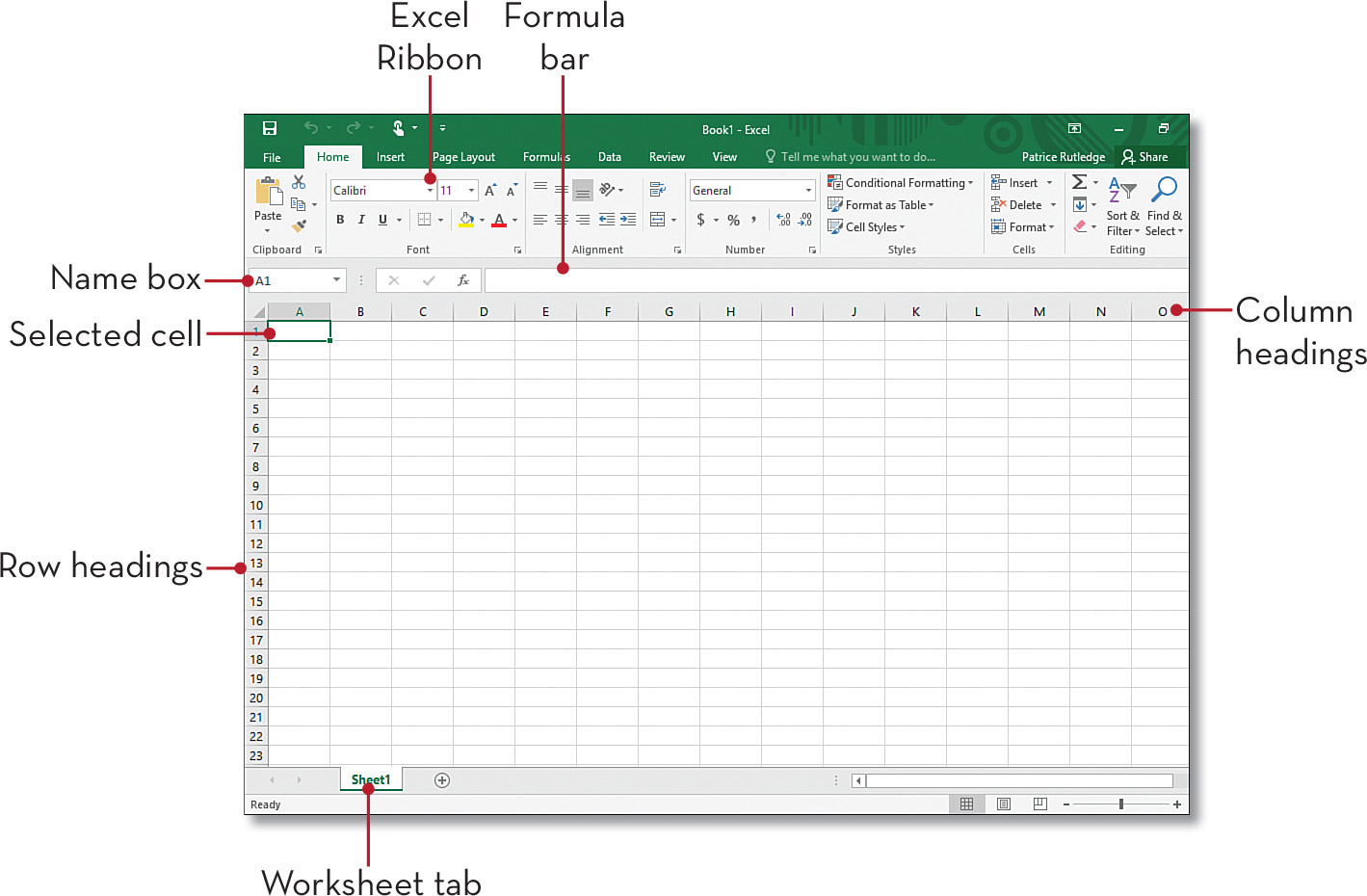
Navigating the Worksheet Screen
You can use your mouse or keyboard to quickly navigate in an Excel worksheet.
![]() Select and drag the vertical scrollbar with your mouse until the row you are looking for is visible.
Select and drag the vertical scrollbar with your mouse until the row you are looking for is visible.
![]() Select and drag the horizontal scrollbar until the column you are looking for is visible.
Select and drag the horizontal scrollbar until the column you are looking for is visible.
![]() Click the wanted cell. It becomes the current cell.
Click the wanted cell. It becomes the current cell.

Note: Cell Address
The name box in the upper-left corner of the screen displays the cell address of the selected cell. A cell address is composed of the column letter and row number, such as cell A1 or cell D8. ![]()
Tip: Other Ways to Navigate a Worksheet
You can also navigate your worksheet using the arrow keys on your keyboard to move one cell at a time up, down, left, or right. Using the Page Up and Page Down keys is another navigation option. If you have a touchscreen device, you can also navigate a worksheet by touch. ![]()
Entering Data
You can enter a variety of data on an Excel worksheet such as numbers, text, dates, or times.
![]() Click the cell where you want to enter data. A border appears around the selected cell.
Click the cell where you want to enter data. A border appears around the selected cell.
![]() Enter your data. A blinking insertion point appears.
Enter your data. A blinking insertion point appears.
![]() Press Enter to accept the value. Excel enters the data into the cell, and the selection moves to the next cell down.
Press Enter to accept the value. Excel enters the data into the cell, and the selection moves to the next cell down.

Tip: Data Entry Option
Optionally, you can press an arrow key instead of the Enter key. This not only accepts the data you entered but also moves to the next cell in the direction of the arrow key at the same time. ![]()
Tip: Entering Sequential Data
If you want to enter sequential data, make your first few entries, select them with your mouse, and then drag the lower-right corner of your selection to have Excel continue entering data. For example, you could enter a series of numbers, days of the week, or months and have Excel finish your work for you. ![]()
Inserting a New Row
Occasionally, you might need to insert a row into the middle of data that you have already entered. Inserting a row moves existing data down one row.
![]() Click the Home tab.
Click the Home tab.
![]() Click the row heading number where you want to insert the new row. Excel selects the entire row.
Click the row heading number where you want to insert the new row. Excel selects the entire row.
![]() Click the Insert button.
Click the Insert button.
![]() Excel moves the existing row down and inserts a new blank row.
Excel moves the existing row down and inserts a new blank row.

Tip: Enter Multiple Rows
To enter more than one row, select the number of rows you want to enter with your mouse, and click the Insert button. For example, if you select rows 7 through 9, Excel moves the existing rows down and inserts three blank rows, numbered 7 through 9. ![]()
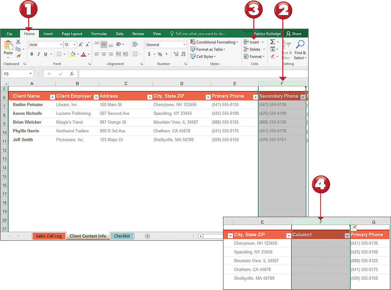
Inserting a New Column
You can also insert a new column on a worksheet with existing data. Inserting a column moves the existing data to the right of the new column.
![]() Click the Home tab.
Click the Home tab.
![]() Click the column heading letter where you want to insert the new column. Excel selects the entire column.
Click the column heading letter where you want to insert the new column. Excel selects the entire column.
![]() Click the Insert button.
Click the Insert button.
![]() Excel moves the existing column to the right and inserts a new column.
Excel moves the existing column to the right and inserts a new column.
Tip: Enter Multiple Columns
To enter more than one column, select the number of columns you want to enter with your mouse, and click the Insert button. For example, if you select columns A through C, Excel moves the existing columns to the right and inserts three blank columns, labeled A through C. ![]()
Deleting Rows and Columns
You can delete Excel rows and columns easily and quickly. Remember that deleting a row or column removes all content from the selected row or column, not just the content of a single cell.
![]() Click the Home tab.
Click the Home tab.
![]() Click the column heading letter or row heading number of the column or row you want to delete.
Click the column heading letter or row heading number of the column or row you want to delete.
![]() Click the Delete button. Excel deletes the selected content.
Click the Delete button. Excel deletes the selected content.

Tip: Delete Multiple Columns or Rows
To delete more than one column or row, select the content you want to delete with your mouse and click the Delete button. For example, if you select the row heading numbers for rows 7 through 9, Excel deletes those rows. ![]()
Inserting a New Worksheet
By default, a new Excel workbook contains a single worksheet named Sheet1. If you like, you can add more worksheets to your workbook. For example, you might want a worksheet for every month of the year, for specific products or projects, and so forth.
![]() Click the plus sign (+) to the right of the Sheet1 tab.
Click the plus sign (+) to the right of the Sheet1 tab.
![]() Excel inserts a new sheet, named Sheet2.
Excel inserts a new sheet, named Sheet2.

Tip: Optional Way to Insert New Worksheets
You can also insert a new worksheet by clicking the down arrow to the right of the Insert button on the Home tab and selecting Insert Sheet from the menu. ![]()
Renaming Worksheet Tabs
Excel names your worksheets consecutively as Sheet1, Sheet2, Sheet3, and so forth. You can easily customize these tab names to something more meaningful, however.
![]() Right-click the tab you want to rename.
Right-click the tab you want to rename.
![]() Select Rename from the menu.
Select Rename from the menu.
![]() Excel highlights the tab name.
Excel highlights the tab name.

![]() Type a new name for the tab, and press Enter to confirm your entry.
Type a new name for the tab, and press Enter to confirm your entry.

Tip: Color a Worksheet Tab
If your workbook has numerous worksheets, you can identify them with colors and labels. To apply a color to a selected worksheet tab, click it, select Tab Color from the menu, and select your preferred color. ![]()
Deleting a Worksheet
If you no longer need a worksheet, or create one by mistake, you can delete it.
![]() Right-click the worksheet you want to delete.
Right-click the worksheet you want to delete.
![]() Select Delete from the menu.
Select Delete from the menu.

Tip: Delete Multiple Worksheet
If you want to delete more than one worksheet, hold down the Ctrl key, and select the worksheets you no longer want. Then, right-click and select Delete from the menu. ![]()
 Caution: Excel Workbooks Require at Least One Worksheet
Because Excel requires at least one worksheet, you can’t delete all the worksheets in your workbook. If you no longer need any of the worksheets in a workbook, you should delete the entire workbook instead. ![]()
Hiding a Worksheet
If you aren’t ready to delete a worksheet, but don’t want it to display in your workbook, you can hide it.
![]() Right-click the tab you want to hide.
Right-click the tab you want to hide.
![]() Select Hide from the menu.
Select Hide from the menu.
![]() Excel hides the tab on the worksheet.
Excel hides the tab on the worksheet.

Tip: Unhide a Worksheet
If you want to display a worksheet again, you can unhide it. To do so, click the Format button on the Home tab, and select Hide & Unhide, Unhide Sheet from the menu. In the Unhide dialog box, you can select the sheet you want to restore. ![]()
Protecting a Workbook with a Password
If your workbook contains confidential information that you want to share only with a select audience, you can protect it with a password. This way, only people who have the password can open the workbook and view its contents.
![]() Click the File tab.
Click the File tab.

![]() Click the Protect Workbook button.
Click the Protect Workbook button.
![]() Select Encrypt with Password from the menu.
Select Encrypt with Password from the menu.

Tip: Make Your Workbook Read-Only
An alternative to protecting your workbook with a password is to make it read-only if you’re more concerned about potential changes than data confidentiality. To make a workbook read-only, select Mark as Final from the Protect Workbook menu. ![]()
![]() In the Encrypt Document dialog box, enter a case-sensitive password for your workbook.
In the Encrypt Document dialog box, enter a case-sensitive password for your workbook.
![]() Click OK.
Click OK.

Tip: Protect Worksheet Data
Another alternative to protecting an entire workbook is to protect specific worksheet data. Doing this enables people to open your workbook but not perform functions you specify, such as format, insert, or delete rows and columns. To protect a worksheet, right-click it and select Protect Sheet from the menu. ![]()