8 Geometry generation and meshing
Abstract: The process of mesh generation, called triangulation, is a key element of numerical experiments due to its essential influence on the accuracy of numerical results. For this reason a good many tools have been developed to construct meshes of appropriate quality relevant to the peculiarities of the problems under consideration. The most popular FOSS grid generators are Gmsh37 and NETGEN38. In addition to meshing procedures, these programs are supplemented with tools for creating simple geometries.
8.1 General information
We need a discrete representation of a computational domain to solve a mathematical model numerically. Mesh generation is the process of creating such a discrete representation of a realistic geometry. This representation must be unique and it is possible that local refinement will be necessary in areas where large gradients of desired functions are suspected. The basic mesh elements are intervals in the 1D case, triangles and quadrangles in the 2 D case, as well as tetrahedrons and hexahedrons in the 3D case.
Two primary classes of meshes are recognized:
- – structured meshes are those with regular connectivity;
- – unstructured meshes have irregular connectivity.
8.1.1 Structured meshes
Structured meshes (Figure 8.1) are widely used in computational mathematics. A structured mesh has a structure with regular connectivity. Advantages of structured meshes are connected to preserving the structure of neighboring nodes and maintaining a certain template for each mesh point. Rectangles (2 D) or parallelepipeds (3D) are usually used as cells in structured meshes. Such meshes are most often employed in finite difference methods.
To generate a regular mesh for a complex geometric object, it is possible to apply a coordinate transformation and construct a uniform grid in the transformed representation of the object. In doing so, the computational mathematical model should be written in the corresponding curvilinear coordinates.

Fig. 8.1. Structured mesh.
8.1.2 Unstructured meshes
The characteristic feature of unstructured meshes (Figure 8.2) is the arbitrary location of mesh points in a physical domain. This arbitrariness should be understood in the sense that there is no special direction of mesh points location, i.e. we do not observe a structure similar to regular meshes. Mesh points may be combined into polygons (2D) or polyhedrons (3D) of arbitrary shape. As a rule, triangle and tetrahedron cells are used in 2D and 3D, respectively. There is usually no need to use more complex cell shapes.
The process of mesh generation is called triangulation. Using a given set of points, a computational domain can be triangulated in various ways. Note that any triangulation method should lead to the same number of cells for the given set of points.
It is often necessary to optimize a generated mesh using certain criteria. The basic optimization criterion is that the triangles obtained should be equilateral (no corner is too sharp). This criterion is local and relates to a single triangle. The second (global) criterion is that neighboring triangles should have equal areas (the uniformity criterion).

Fig. 8.2. Unstructured mesh.
A special triangulation does exist, i.e. a Delaunay triangulation, which has a number of optimal properties. First, the triangles generated tend to be equilateral, i.e. the Delaunay algorithm maximizes the minimal interior angle of mesh triangles. The second property is that a circle circumscribing any triangle does not include any other points in its interior. A more detailed description of the properties of a Delaunay mesh can be found in the specialist literature. We now introduce a Voronoi diagram (partition) and its connection with Delaunay triangulations for further discussion.
A Voronoi diagram for any point (named a seed) is a set of points located closer to this point than to any other. A cell of Voronoi diagrams is obtained from the intersection of half spaces bounded by the perpendicular to the midpoint of the segment joining the two nearest points. It should be noted that Voronoi cells are always convex polygons.
Each vertex of a Voronoi diagram is the meeting point of three Voronoi polygons. Seeds of these polygons form a Delaunay triangulation. Thus, we have dual consistency between Delaunay triangulations and Voronoi diagrams.
Delaunay triangulations are actively employed for the numerical solution of applied problems on the basis of finite element methods. There are many well-developed methods and software for generating such triangle meshes. As mentioned above, we will now consider two of the most popular tools.
8.2 The Gmsh workflow
Two programs for generating 3D meshes are considered here. Namely, Gmsh and NETGEN, which are commonly used to construct 3D meshes. As a rule, CAD (computer-aided design) systems are employed to create complex geometrical models. These two programs also allow us to build simple geometrical models.
To install Gmsh, we can download it from the official website listed above (for Windows, Linux and Mac), or for the Ubuntu operating system we can apply the command below.
8.2.1 Elementary entities
Gmsh is an automatic mesh generator for 2D and 3D domains. It has a light and user-friendly graphical interface. Gmsh consists of four modules which deal with geometry, mesh, solver, and post-processing (Figure 8.3).
To launch Gmsh in the interactive mode, we should click on the program icon or use the command

Fig. 8.3. Gmsh.
A geometry is created in Gmsh using elementary entities, i.e. points, lines, surfaces, and volumes. The constructed geometry is saved as a geo-file. A geo-file can also be created and edited using any text editor, and can then be loaded by the File | Open menu command. The file can also be edited in the Geometry module, by clicking the Edit button.
The Geometry module provides the possibilities of a simple CAD system and employs a boundary representation (BRep) to define geometric objects. In order to describe geometries, we first define points (using the Point command), then introduce lines (the Line, Circle, Ellipse, and spline commands), and surfaces (the Plane and Ruled Surface commands), and finally describe volumes (the volume command). These geometric entities have an identification number, which is assigned to them at creation. We can also move and modify geometric entities via the Translate, Rotate, Dilate or Symmetry commands.
These entities are considered in detail in the following.
Point:
Point(id) = {x, y, z, size}.
Creates a point with the identification number (id). The three x, y, and z coordinates of the point and the prescribed mesh element size are specified inside the brackets. The last argument is optional.
- – Line(id) = {pointId1, pointId2}.
Creates a straight line with the identification number (id). The start and end points of the line are given identification numbers inside the brackets.
- – Circle(id) = {pointId1, pointId2, pointId3}.
Creates a circle arc (strictly smaller than π) with the identification number (id). The identification numbers of the start, center, and end points of the arc are given inside the brackets.
- – Ellipse(id) = {pointId1, pointId2, pointId3, pointId4}.
Creates an ellipse arc with the identification number (id). Inside the brackets pointId1 and pointId2 are the identification numbers of the start and center points of the arc, respectively, pointId3 is the identification number of any point located on the major axis of the ellipse, pointId4 is the identification number of the end point of the arc.
- – Line Loop(id) = {lineId1, lineId2, ..., lineIdN}.
Creates a closed line loop with the identification number (id). Inside the brackets, we set a list of identification numbers of all the lines which compose the loop.
Surfaces:
- – Plane Surface(id) = {lineLoopId1, lineLoopId2, ..., line} LoopIdN}.
Creates a plane surface with the identification number (id). Inside the brackets we give a list of identification numbers of all line loops which define the surface. The exterior boundary is defined by the first line loop and all other line loops specify holes in the surface.
- – Ruled Surface(id) = {lineLoopId1, lineLoopId2, ..., line LoopIdN}.
Creates a ruled surface similar to plane surfaces;
- – Surface Loop(id) = {surfaceId1, surfaceId2, ..., surface IdN}.
Creates a surface loop (a closed shell) with the identification number (id). Inside the brackets we provide a list of identification numbers of all surfaces which constitute the loop.
Volume:
Volume(id) = {surfaceLoopId1, surfaceLoopId2, ..., surface LoopIdN}.
Creates a volume with the identification number (id). Inside the brackets we give a list of identification numbers of all surface loops which compose the volume.
8.2.2 Commands for working with geometric objects
Lines, surfaces, and volumes can also be created using the Extrude command.
- – Extrude{x, y, z} {object}.
Extrudes an object along the vector. Inside the first brackets we give the coordinates of the vector (x, y, z). Objects can be points, lines, or surfaces.
- – Extrude{{x1, y1, z1}, {x2, y2, z2}, angle} {object}.
Extrudes an object with a rotation. Inside the first brackets we specify the directions of the rotation axis (x1, y1, z1), the coordinates of a point on this axis (x2, y2, z2), and the rotation angle in radians (angle).
- – Extrude{{x1, y1, z1}, {x2, y2, z2}, {x3, y3, z3}, angle} {object}.
Extrudes an object along the vector with a rotation. Inside the first brackets we give the coordinates of the vector (x1, y1, z1). Other arguments are the same as in the previous case.
We can apply geometrical transformations to elementary entities or to their copies created by the Duplicata command.
- – Rotate{{x1, y1, z1}, {x2, y2, z2}, angle} {object}.
Rotates an object (points, lines, surfaces or volumes) by an angle (in radians). Inside the first brackets we specify the directions of the rotation axis (x1, y1, z 1). The coordinates of a point on this axis (x2, y2, z2) are specified. To rotate the copy of the object, we must use Duplicata {object}.
- — Translate{x, y, z} {object}.
Translates an object along the vector (x, y, z).
- – Symmetry{A, B, C, D} {object}.
Moves an object symmetrically to a plane. Inside the brackets we set the coefficients of the plane’s equation (A, B, C, D).
- – Dilate{{x, y, z}, factor} {object}.
Scales an object by a factor. Inside the brackets we give the directions of the transformation (x, y, z).
8.2.3 Physical entities
The major advantage of Gmsh is the existence of physical entities. These entities are employed to unite elementary entities into larger groups. They can be used to set boundaries and sub-domains of a future mesh.
- – Physical Point(id) = {PointId1, PointId2, . . . , PointIdN}.
Creates a physical point with the identification number (id). Inside the brackets we set a list of elementary points which need to be grouped into one group.
- – Physical Line (id) = {LineId1, LineId2, . . . , LineIdN}.
Creates a physical line with the identification number (id). Inside the brackets we specify a list of elementary lines which need to be grouped into one group.
- – Physical Surface(id) = {SurfaceId1, SurfaceId2, ... , SurfaceIdN}.
Creates a physical surface with the identification number (id). Inside the brackets we present a list of elementary surfaces which need to be combined into one group.
- – Physical Volume(id) = {VolumeId1, VolumeId2, ... , VolumeIdN}.
Creates a physical volume with the identification number (id). Inside the brackets we set a list of elementary volumes which need to be grouped into one group.
Note that the identification number of a group can be either a number or a string. In the latter case, a number will be given automatically.
8.2.4 Building geometry
We now consider an example of building a 2D domain. We create a mesh. geo file using any text editor. First, we define auxiliary parameters as follows:

Here, p1 and p2 are mesh element sizes and r is a radius. Next we create points to define a rectangle and circle as outlined below:

Straight lines and circle arcs are then introduced as follows:


along with a plane surface:

Further, we open the obtained mesh. geo file in Gmsh. Figure 8.4 shows the designed geometric domain.

Fig. 8.4. 2D geometric domain.
Finally, we can transform our 2D domain (Figure 8.4) into the 3D box presented in Figure 8.5 using the following Extrude command:


Fig. 8.5. 3D geometric domain.
8.2.5 Tools
Gmsh provides an extensive set of tools which accelerate building geometric domains. We now discuss the most useful ones.
- – Arithmetic operations.
Gmsh supports all basic arithmetic (=, +, -, *, /, ^, %, +=, += , – = , *= , / = , ++, --), relational (>, >=, <, <=, ==, ! =), and logical operations (&&, | |, ! ). All of these operations correspond to similar operations in C/C++.
- – Built-in functions.
Gmshprovidesbuilt-inmathematical functions: Sin, Cos, Tan, Exp, Fabs, Log, Log10, Sqrt, etc.
- – User-defined functions.
Users can also introduce their own functions to perform certain operations. A function is defined using the Function function_name command. The function must be closed by the Return command. The body of functions contains any number of operations. Note that the function does not take any arguments, i.e. it uses only global variables. The function can be called by the Call function_name command.
- – Loop.
Loops are defined using the For var In (start, end, step) command. Here the value of the variable var iterates from the value of start to the value of end with the step increment. The last parameter can be omitted; in this case, the step is taken to be unity. The loop must end with the EndFor command.
- – Conditionals.
Conditional operators begin with the If (condition) command and end with the EndIf command. The number of operations performed is not limited for the correct condition.
- – Comments.
To aid in the understanding Gmsh script files, comments can be employed which have the C/C++ style, i.e. // for single-line comments and / * and * / for block comments.
8.2.6 Creating a complex geometry
An example of creating the 3D box depicted in Figure 8.5, with n layers using the tools mentioned above, is now presented.
First, we create the plane. geo file, where we define a function that builds a unit square with a circle with a radius r (Figure 8.4).

Here newp, newl, new11, and news return the next available number of points, lines, line loops, and surfaces, respectively. We store the numbers of points, lines and surfaces in arrays to work with them later. The number of our plane is i, z defines a position of the plane on the z axis, whereas h1 and h2 are mesh element sizes.
Next, we create the mesh-3d. geo file and include plane. geo in the file.
Now we can apply the plane function in our script.
We define geometry parameters as follows:


Fig. 8.6. Planes created by loop.
Using the loop operator For, we create n+1 planes (Figure 8.6).

Next, we must connect the points of the plane i ! = 1 with the corresponding points of the plane i – 1 by lines. For this, we employ the conditional operator If.

Combining all the lines in the plane, we create layers as demonstrated in Figure 8.7.
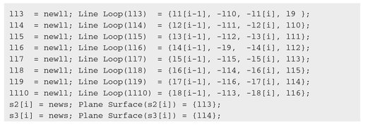

Here news 1 and newv return the next available number of surface loops and volumes, respectively.
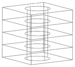
Fig. 8.7. 3D box with 4 layers.
We must close the the If and For operators:

Now we create physical groups to define boundaries (Figure 8.8) as follows: and layers (Figure 8.9).


Fig. 8.8. Boundaries.

Fig. 8.9. Layers.

8.2.7 Generating a mesh
We use the 1D, 2D, and 3D buttons in the Mesh module to generate a mesh. We can also generate a mesh non-interactively in the batch mode without using the graphical interface as follows:

Fig. 8.10. 3D mesh.

Fig. 8.11. 2D mesh.
This command generates a 3D mesh of the domain defined in the mesh. geo file; see Figure 8.10. The 2D mesh is generated if we apply the –2 option (Figure 8.11).
A generated mesh can be saved in an msh-file by clicking the Save button. In addition, we can save a mesh in different formats using the File | Save As menu command.
It is possible to refine the mesh generated by clicking the Refine by splitting button (Figure 8.12), or using the -refine option in batch mode as follows:
Here we saved the refined mesh in the meshRefined.msh file via the – o option.
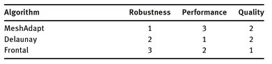
Gmsh includes the following meshing algorithms:
- – MeshAdapt is an algorithm based on local mesh modifications. It is suitable for generation of 2D meshes.

Fig. 8.12. Refined 2D mesh.
- – Delaunay is the well-known algorithm based on the Delaunay criterion.
- – Frontal is a method based on the Bowyer-Watson algorithm.
These algorithms can be selected by adding the following command in a script file:
for 2D meshes and
for 3D meshes. Here a number represents the selected algorithm. For the 2D case, we have: 1 is MeshAdapt, 2 denotes Automatic, 5 is Delaunay, and 6 indicates Frontal algorithm, respectively; for 3D meshes, 1 corresponds to the Delaunay and 4 indicates Frontal algorithm, respectively.
Algorithms can be changed using the Tools | Options | Mesh | General menu command. In the batch mode, algorithms are defined as follows:
Table 8.1 presents the ranking of algorithms with respect to robustness, performance, and quality.
Gmsh makes it possible to save meshes in many formats supported by well-known finite element packages. Here, we describe an msh-file presented in the basic file format of Gmsh.
The msh-file consists of one mandatory section with information about the file (MeshFormat), and optional sections describing nodes, elements, and more.
Table 8.1. Features of 2D mesh generation algorithms.
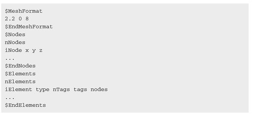
Here nNodes is the number of nodes, iNodes is the node index, x, y, z are the coordinates of the node, nElements is the number of elements, iElements is the element index, type is element type (Table 8.2), nTags is the number of tags, tags is a list of tags, and nodes is a list of nodes which compose elements.
Table 8.2. Element types.
| Number | Type |
|---|---|
| 1 | line |
| 2 | triangle |
| 3 | quadrangle |
| 4 | tetrahedron |
| 5 | hexahedron |
By default, msh-files has three tags. The first tag is the number of the physical group, the second defines the number of the elementary geometrical entity, and the third tag sets the number of mesh partitions.
8.3 NETGEN first look
NETGEN is another automatic 3D mesh generator (Figure 8.13). The program is also an open source tool distributed under the conditions of the LGPL license.

Fig. 8.13. NETGEN.
To install NETGEN, we can download the executable file for windows from the project’s website listed above or source code. In Ubuntu, it is possible to use the following command:
8.3.1 Creating a geometry
NETGEN is invoked in the interactive mode by clicking on the program icon or using the command below.
In NETGEN, a geometric model is created employing the constructive solid geometry format (CSG). It is defined in an ASCII-format file using any text editor.
The following basic geometric primitives are available:
- – plane(px, py, pz; nx, ny, nz).
A half-space defined by a plane. A plane is defined by an arbitrary point (px, py, pz) and an outside normal vector (nx, ny, nz).
- – cylinder(ax, ay, az; bx, by, bz; r).
An infinite cylinder. It is described by two points (ax, ay, az) and (bx, by, bz) on the central axis, and by the radius r.
- – sphere(cx, cy, cz; r).
A sphere. It is defined by the center (cx, cy, cz) and the radius r.
- – ellipticcylinder(cx, cy, cz; vx, vy, vz; wx, wy, wz).
An elliptic cylinder. It is specified by the point (cx, cy, cz) on the major axis, and the vectors (vx, vy, vz), and (wx, wy, wz) of the long and short axis of the ellipse, respectively.
- – ellipsoid (cx, cy, cz; ux, uy, uz; vx, vy, vz; wx, wy, wz).
An ellipsoid. It is defined by the center (cx, cy, cz), and the vectors (ux, uy, uz), (vx, vy, vz), and (wx, wy, wz) of the main axis of the ellipsoid.
- – cone(ax, ay, az; ra; bx, by, bz; rb).
A cone. It is described by the two points (ax, ay, az) and (bx, by, bz), and the corresponding two radii ra and rb.
- – orthobrick (ax, ay, az; bx, by, bz).
An orthobrick. It is defined by the two opposite corner points (ax, ay, az) and (bx, by).
Now we present an example of building a 3D domain. First, we create the mesh. geo o file using any text editor and build an orthobrick and a cylinder as follows:
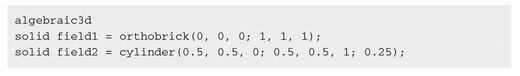
The keyword algebraic3d is mandatory. Next, we apply a boolean operation to cut the cylinder from the orthobrick.
Using the keyword tlo (top-level-object), we declare the 3D domain for meshing.
We load the geo-file using the File | Load Geometry menu command or the command
8.3.2 Generating a mesh
To generate a mesh we need to click the Generate Mesh button or run NETGEN in the batch mode as follows:
This command generates a mesh of the domain specified in the mesh.geo file and saves it in the out. mesh file. The mesh can be stored in other formats associated with various finite element packages and mesh generators. Thus, to save the mesh in the msh-file for Gmsh, we apply the –meshfiletype=“Gmsh2 Format” option to specify the necessary file format, and the -meshfile=mesh.msh option to change the file name.
The quality of a mesh can be controlled using the -verycoarse, -coarse, –moderate, –fine, –veryfine options in the batch mode or the Mesh | Meshing Option | General | Mesh granularity menu command in the interactive mode.
Figure 8.14 shows the 3D mesh specified above.

Fig. 8.14. 3D domain in NETGEN.