11.1.1 Mathematical model

A mathematical model describing temperature distribution with phase transition between solid and liquid phases at some given phase transition temperature T* in a domain Ω = Ω^- u Ω⁺ ∪ S is presented below.

Here Ω⁺(t) is a domain occupied by the liquid phase (melted zone), where the temperature is higher than the phase transition temperature

and Ω^-(t) is a domain occupied by the solid phase (frozen zone)

The phase transition takes place at the phase interface S = S(t) (Figure 11.1).

We use the classic Stefan model, which describes thermal processes accompanied by phase transformations, as well as latent heat absorption and release, for modeling heat transfer processes with phase changes:

(11.1)

where L is the specific heat of phase transition.

Fig. 11.1. Computational domain.

We have the following relations for the equation coefficients:

where ρ⁺, c⁺ and ρ^-, c^- are the density and specific heat capacity of melted and frozen zones respectively.

As we are considering the process of heat distribution in a porous medium, we have the following coefficients:

where m represents porosity. The sc, w, i indexes denote soil skeleton, water, and ice respectively.

We have similar relations for the thermal conductivity coefficients in the melted and frozen zone:

In practice, a phase transition does not happen instantly and can occur within a small temperature interval [T* - Δ, T* + Δ]. As the function ϕ, we take ϕ_Δ

In this case, we obtain the following equation for the temperature in the domain Ω:

(11.2)

The equation (11.2) is the standard nonlinear parabolic equation.

The equation (11.2) is supplemented with the initial

(11.3)

and boundary conditions

(11.4)

Here Γ₁ is an interface with a freezing canal.

11.1.2 Finite element discretization

Discretization of the problems (11.2)-(11.4) in space is carried out via the finite element method. On multiplying the temperature equation by a test function v and integrating by parts, we obtain

(11.5)

Here

where H(Ω) is the Sobolev space consisting of functions v such that _V² and |∇v|² have finite integrals over Ω.

For simplicity, we define a uniform time grid thus:

and apply the standard backward Euler (fully implicit) scheme for time-stepping. We use the simplest linearization where coefficients depend on the previous time level value of the function to linearize the equation:

(11.6)

where T“ = T(tⁿ) ∈ V. In order to perform calculations, we must go from the continuous variational problem (11.6) to a discrete one. In doing so, we introduce finite dimensional spaces V_h, ⊂ and define the following problem: find T_h ∈ V_h, such that

(11.7)

where . Note that the choice of the space follows directly from the type of finite elements used.

11.1.3 Numerical implementation

Let us consider a problem in 2D formulation. Due to the peculiarities of FEniCs, making the transition to 3D formulation is no problem.

The process of numerical solution consists of the following steps:

• – building a geometry and generating meshes;
• – the numerical implementation of the constructed algorithm in FEniCS;
• – visualizing obtained results.

To build a 2D geometrical model and generate a mesh using the previously discussed Gmsh, we define the geometry of our domain in the following geo-file:

We open this file in Gmsh and click the 2D button (if necessary we can refine our meshes) to generate a mesh. Next, we save the generated mesh in the msh format in the rock.msh file. To use this mesh in FEniCs, we convert it by applying the dolfin-convert utility.

The implementation of the computational algorithm is performed by means of FEniCS. We describe our problem in the Temperature. ufl file, where we define the bilinear and linear forms of the variational formulation (11.7):

From Temperature. ufl, using the command

we generate the Temperature. h file to use in the main program.

The program for calculations is written in c++. In the main. cpp file, we include the dolfin. h library and generated header file Temperature. h:

Listing 11.1.

We create the computational mesh from the rock. xml file as well as the mesh function with boundary part marks from the rock_facet_region. xml file:

Listing 11.2.

Next, we define the function space for the temperature:

Listing 11.3.

Further, we create the functions T and T0:

Listing 11.4.

The latter function is used to store the value corresponding to the previous time level.

Now we define constants for the time step, the temperature of the freezing canal, and various coefficients of the equation:

Listing 11.5.

We create the Dirichlet boundary condition using the mesh function, where we specify the temperature of the freezing canal:

Listing 11.6.

Then we define the initial temperature distribution:

Listing 11.7.

Next, we create the bilinear and linear forms and prescribe their coefficients:

Listing 11.8.

To solve the problem, we should define the matrix, the vector on the right and the linear solver. Here we choose the gmres method with the ilu (default) preconditioner:

Listing 11.9.

To visualize the results, e.g. in ParaView, we will save them as a vtk file:

Listing 11.10.

We use the time loop with the constant time step for integration in time:

Listing 11.11.

Further, we assemble the matrix and vector, apply the boundary condition to them, and calculate the temperature:

Listing 11.12.

The results of the current time level are written in the file:

Listing 11.13.

At the end of the loop, the value of the current time level is assigned to the value of the previous time level, and we move to the next time level:

Listing 11.14.

11.1.4 Predictions

Here we present the results of the numerical simulation of the artificial freezing process. Calculations are conducted in the geometrical domain which is 2 meters long in both directions. The freezing canal has a radius of 0.1 meter and is located on the right of the domain. The computational mesh consists of 15,064 triangle cells. The time step is τ = 0.1 day. The temperature distribution after 1, 10, and 30 days is shown in Figure 11.2.

Fig. 11.2. Temperature distribution after 1,10, and 30 days (from left to right).

It is interesting to compare the zero isotherms (T = 0) obtained on three computational meshes with (a) 920, (b) 3,768, and (c) 15,064 cells presented in Figure 11.3.

Fig. 11.3. Meshes. From left to right: (a) 920; (b) 3,768; (c) 15,064.

Below, we present a comparison of the temperature dynamics (the isotherm T = 0 after various periods of time: 1, 5, 10, 20, 30 days) for different values of the time step τ (Figure 11.4). Calculations are performed for Δ = 1 using the mesh with 15,064 cells. The value of the time step greatly affects the solution error; calculation with the minimal time step τ = 0.1 gives the most accurate solution.

Fig. 11.4. Comparison of the temperature for different moments (in days) with different time steps r: 0.1 (blue), 0.25 (green), and 0.5 (red).

The effect of smearing the phase transition on the error of the solution is shown in Figure 11.5. The comparison is performed for the mesh with 15,064 cells and τ = 0.1 day. It is easy to observe that the large interval of smearing leads to a loss of accuracy.

Fig. 11.5. Comparison of the temperature for different moments (in days) with different Δ: 1.0 (blue), 1.5 (green), and 2.0 (red).

Figure 11.6 demonstrates the influence of mesh size on the error of the solution. The calculations are performed for τ = 0.1 day and Δ = 1. The figure illustrates the convergence of the solution by refining the computational mesh.

Fig. 11.6. Comparison of the temperature for different moments (in days) with different meshes: 920 cells (blue), 3,788 cells (green), and 15,064 cells (red).

11.2.1 Incompressible Navier-Stokes equations

In the domain Ω presented in Figure 11.7, we consider a fluid flow governed by the Navier-Stokes equations:

(11.8)

Here u(x, t) is the velocity and p(x, t) stands for the pressure. As for the Reynolds number

v is the reference value of the velocity, L is the length of the square cavity walls, and v denotes the kinematic viscosity. The Reynolds number is a dimensionless value defining the ratio of nonlinear and dissipative terms. Flow behavior changes essentially depending on its value. Thus, if the Reynolds number is more than the critical value, flow becomes turbulent instead of laminar.

We set nonzero velocity to bring the fluid into motion at the rigid top of the cavity Γ₁. Other boundaries of the cavity Γ₂ are fixed rigid walls, i.e. no-slip and no-permeability conditions are imposed on them. Therefore, we supplement our system (11.8) with the following boundary conditions:

(11.9)

Fig. 11.7. Computational domain.

Finally, we specify the initial conditions:

11.2.2 Variational formulation

There are many methods to approximate the system of equations in time (11.8). For simplicity, we define a uniform time grid

Here we employ the Douglas-Rachford splitting scheme with nonlinear coefficients taken from the previous time level:

(11.10)

(11.11)

(11.12)

We calculate uⁿ⁺¹ and pⁿ⁺¹ at the current time level in three steps:

• – calculate the intermediate velocity;
• – evaluate the new pressure pⁿ⁺¹;
• – compute the final velocity uⁿ⁺¹.

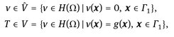
Let us rewrite these problems in variational forms. For velocity, we define the Sobolev space V(Ω), consisting of vector functions u such that u², (div u)² , and |grad u|² have finite integrals over Ω:

where g is the Dirichlet boundary condition. Similarly, we define the following space for pressure:

On multiplying (11.10) by the test function v and integrating by parts, we get the variational problem: find u* ∈ V such that

(11.13)

Next, we subtract (11.10) from (11.11) and take the divergence:

Since div uⁿ⁺¹ = 0, the term with uⁿ⁺¹ disappears. By multiplying the obtained equation by the test function q and integrating over Ω, we arrive at the problem: find pⁿ⁺¹ ∈ Q such that

(11.14)

We again subtract (11.10) from (11.11). Next, we multiply the resulting equation by v and integrate over the domain. We arrive at the problem: find uⁿ⁺¹ ∈ V such that

(11.15)

To go from variational problems (11.13)–(11.15) to discrete ones, we define the finite dimensional spaces V_h, , Q_h, and contained in V, , Q, and , respectively.

First, we search such that

(11.16)

The second discrete problem is to find such that

(11.17)

And finally, find such that

(11.18)

As for the spaces V_h and Q_h, we use the standard Lagrange spaces of second and first order, respectively.

11.2.3 Numerical algorithm

Gmsh is employed to create a 2D geometrical model and generate meshes. The geometry of our domain is written in the file cavity. geo:

For further application, we convert the obtained mesh using dol fin-convert:

The numerical algorithm is implemented using FEniCS. The problem statement is described in the file step. ufl, where we define linear and bilinear forms from (11.16)- (11.18):

From this ufl-file, we generate a class to apply it in the main source code:

As usual, the program is written in the C++ programming language. We include the library dolfin. h and the header file step. h generated above in this program:

Listing 11.15.

Next, we create the computational mesh from the file cavity.xml, and the mesh function with boundary marks from the file cavity_facet_region. xml:

Listing 11.16.

We then define spaces for velocity and pressure:

Listing 11.17.

We initialize the function for the previous time level u0, p0, for intermediate velocity ut, and unknown functions u and p:

Listing 11.18.

We should specify constant values for the time step tau, Reynolds number Re, boundary conditions onezero, and zerozero:

Listing 11.19.

Further, we create the Dirichlet boundary conditions:

Listing 11.20.

We introduce the bilinear and linear forms and preset their coefficients:

Listing 11.21.

Next, it is necessary to define matrices and vectors of linear systems. We also specify linear solvers which use the gmres method with the default preconditioner:

Listing 11.22.

The VTK format is chosen to save computed results for further post-processing:

Listing 11.23.

The loop in time with the constant time step is arranged for the time-integration.

Listing 11.24.

We calculate the intermediate velocity after assembling the matrix and vector and applying boundary conditions:

Listing 11.25.

Next, we evaluate the new pressure. Note that we do not apply any boundary conditions:

Listing 11.26.

And finally, we compute the final velocity:

Listing 11.27.

After this, we write the results into the files:

Listing 11.28.

We assign the value of the current time level to the functions corresponding to the previous time level and move to the next time level.

Listing 11.29.

11.2.4 Computational experiments

The results of numerical experiments for this fluid flow problem are presented below. Calculations are conducted using the mesh with 3,794 cells (see Figure 11.8) and the time step τ = 0.01. The final time is T = 20.

Fig. 11.8. Computational mesh.

The velocity vector field for Re = 1000 at the final moment treated as the steady-state solution is shown in Figure 11.9. The velocity components are depicted in Figure 11.10.

We employ the Stream Tracer With Custom Source filter of ParaView to show streamlines. The process of vortex formation for Re = 1000 is shown in Figure 11.11 for different moments in time.

The velocities at the final time t = 20 for different Reynolds numbers 10, 100, and 1000 are presented in Figure 11.12. It is easy to see that an increase of the Reynolds number changes vortex behavior due to the greater influence of convective terms of the Navier-Stokes equations.

Fig. 11.9. Velocity vector field.

Fig. 11.10. Velocity components.

Fig. 11.11. Streamlines for Re = 1000 at different moments.

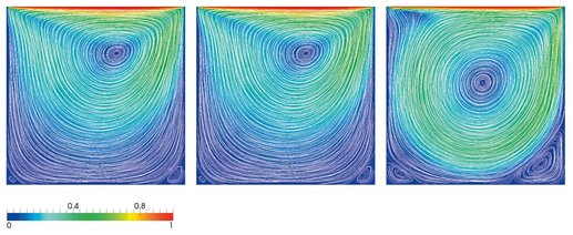
Fig. 11.12. Streamlines for Re = 10, Re = 100, Re = 1000 (from left to right).

11.3.1 Governing equations

Displacement u, strain ε, and stress σ occur in an elastic body under mechanical and thermal effects. External (surface or volume) forces which impact the body are treated as mechanical effects, whereas for thermal influences, we mean heat exchange processes between the body surface and environment, and release or absorption of heat by the sources inside the body.

Fig. 11.13. Computational domain.

The mathematical model of the thermoelastic state of the body in a domain Ω = Ω₁ ∪ Ω₂ involves the following coupled system of equations for the displacement u and temperature T:

(11.19)

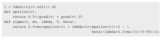
Here µ, λ, denote Lame constants, k is the heat conduction coefficient, T₀ stands for the constant absolute temperature at which the body is in an initial state of equilibrium, and α = α_T(3λ + 2µ), where α_T is the linear thermal expansion coefficient.

Let us supplement equations (11.19) with appropriate boundary conditions for temperature:

(11.20)

where T_air is the ambient temperature and y denotes the convective heat transfer coefficient.

As for boundary conditions for the displacement, we define the point fixation, i.e. in the upper lefthand corner

in the upper righthand corner

and the remaining surfaces are free σ = 0.

11.3.2 Finite element technique

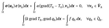
It is necessary to create a finite element discretization in space to numerically solve the problem (11.19)-(11.20). We integrate the equations over the domain Ω and apply Green’s formula, which results in

(11.21)

where

where H(Ω) is the Sobolev space.

We proceed from the continuous variational problem (11.21) to the discrete one. Let us define the finite-dimensional spaces V_h ⊂ V, Q_h ⊂ Q and and formulate a discrete problem on them: find T_h ∈ Q_h, u_h, ∈ V_h such that

(11.22)

As for spaces V_h and Q_h, the standard spaces of Lagrange polynomials of the second and first degree, respectively, are used.

11.3.3 Algorithm of calculations

The problem being considered is solved using the finite element platform FEniCS. We use the Gmsh software to build a 2D geometrical model and generate a mesh. The geometry of the computational domain is defined by the following geo-file:

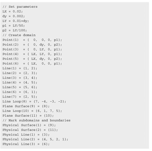
We generate the computational mesh block. msh from the file block. geo, and then convert it to the xml format using the dol fin-convert utility.

The variational formulation of the problem is described in the file ThermoElasticity. ufl, where we define bilinear and linear forms for displacement, temperature and stress. At the beginning, we introduce spaces to search for functions:

Let us define constants for the coefficients of equations and boundary conditions:

Functions are also introduced for deformation and stress:

The functions T and q, bilinear and linear forms for temperature are defined as

Also, the functions u and v are introduced for displacement evaluation and bilinear and linear forms are specified:

We define the necessary functions and forms to compute the arising stresses:

From the file ThermoElasticity. ufl by calling the command

we generate the file ThermoElasticity. h to import into the main program.

For the numerical solution, we include dolfin.h library, the header file ThermoElasticity.h generated earlier and define the class PinPoint for (the upper left and right) point allocation to define Dirichlet boundary conditions on them:

Listing 11.30.

We create an object for the computational grid from the block.xml file, an object with marks for computational domain boundaries and the file containing subdomains marks:

Listing 11.31.

Next, we introduce spaces for the temperature and displacement:

Listing 11.32.

We create the unknowns T and u:

Listing 11.33.

Further, we define equation coefficients and boundary condition parameters:

Listing 11.34.

It is necessary to specify Dirichlet boundary conditions for displacement (the upper left and upper right points of fixation) and for temperature (a constant temperature on the upper and lower boundaries):

Listing 11.35.

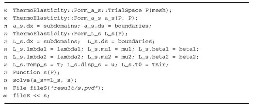
Next, we create objects for bilinear and linear forms and indicate necessary objects of functions or constants:

Listing 11.36.

We create objects for matrices and vectors and define linear solvers (by default, it is the direct ILU-factorization method):

Listing 11.37.

Further, we assemble matrices and vectors, apply Dirichlet boundary conditions and calculate temperature and displacement:

Listing 11.38.

For visualization of the following results, function values are saved in vtk-format, which can be visualized using the ParaView program:

Listing 11.39.

For visualization of the arising stresses, functions and forms (bilinear and linear) are defined and the results are saved in the file:

Listing 11.40.

11.3.4 Numerical results

We now discuss the numerical results of the above problem. Computations were carried out for a plate 0.02 meters long and consisting of two layers 0.01 and 0.002 meters thick, respectively. The computational grid depicted in Fig. 11.14 has 21,952 triangular cells.

Fig. 11.14. Computational grid.

Distributions of temperature and displacements are presented in Figures 11.15, 11.16, and 11.17, respectively. Arising stresses are shown in Figure 11.18.

Fig. 11.15. Temperature distribution.

Fig. 11.16. Displacement distribution along the x axis.

Fig. 11.17. Displacement distribution along the y axis.

Fig. 11.18. Stress distribution (von Mizes) along the x direction (from left to right).

11.4.1 Problem formulation

Let us consider a problem of electric current flowing through a conductor, where heat loss is significant due to current transmission. On the one hand, increasing the conductor temperature is governed by the Joule heating law; on the other hand, the electrical properties of the conductor depend on the temperature.

We consider stationary electric fields, which are induced by currents flowing in a continuum. Let j = j(x) be the electric current density at the point x. This field satisfies the equation

(11.23)

For the electric field intensity E, we have

(11.24)

These equations must be supplemented by a relation which couples j and E. From Ohm’s law for an immobile medium, we get

(11.25)

where σ is the electrical conductivity coefficient.

According to (11.24), the electric field has a potential, and it is therefore possible to describe it introducing the potential φ such that

(11.26)

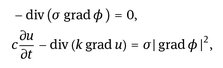
Substituting (11.26) in (11.25) and taking (11.23) into account, we get the elliptic equation for electric potential:

(11.27)

Here

where u is the temperature.

The time-dependent temperature field is governed by the equation

(11.28)

where c is the volumetric heat capacity of a conducting medium and k stands for the heat conduction coefficient.

When current flowing through a conductor generates heat, the value at a particular point depends on the current and electric field intensity and equals (Joule’s law):

(11.29)

Therefore, the system of equations describing thermoelectric processes may be written in the following form:

(11.30)

for x ∈ Ω, Ω = Ω₁ ∪ Ω₂ and t ∈ [0, T] (see Figure 11.19).

The system of equations (11.30) is supplemented with the initial

Fig. 11.19. Computational domain.

and the boundary conditions for the temperature:

as well as boundary conditions for the potential:

Here Γ_D is the boundary, where potential is defined (Γ_D = Γ₁ ∪ Γ₆), Γ_R denotes the boundary that exchanges heat with the environment, T_air is the air temperature of the environment, and α stands for an empirical coefficient of heat transfer (Γ_R = Γ₁ ∪ Γ₂ ∪ Γ₃ ∪ Γ₄).

11.4.2 Discrete problem

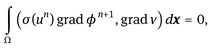
We need to perform discretization of the system of equations (11.30) using the finite element method. Multiply the potential equation by the test function v and integrate using Green’s formula; this results in the equation

(11.31)

Similarly, by multiplying the temperature equation by the test function q and integrating it over the computational domain, we get

(11.32)

Here

where H(Ω) is the Sobolev space consisting of functions v such that _V² and |∇v|² have finite integrals over Ω.

We apply the backward Euler (fully implicit) scheme to approximate the temperature equation in time.

(11.33)

(11.34)

Now we must proceed from the continuous variational problem (11.33)-(11.34) to the discrete one. We introduce finite-dimensional spaces V_h ⊂ V, Q_h ⊂ Q and , , and define the discrete problem on them: find u_h, ∈ Q_h, φ_h ∈ V_h, such that

(11.35)

(11.36)

As for spaces V_h and Q_h, we use default Lagrange polynomial spaces.

11.4.3 Computational algorithm

We build a computational domain and generate a mesh using the Gmsh software to solve the above problem numerically. The computational domain is 5 mm long in both directions and includes the domain Ω₁ as the electricity conducting element, which is 1 mm thick and 2 mm long. Next is the cup, which is 0.3 mm thick, and the domain Ω₂ occupied by a conducting fluid which is heated by passing the electric current through it:

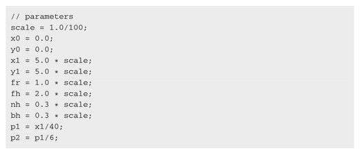
The domain is built by setting dots and lines to define surfaces:

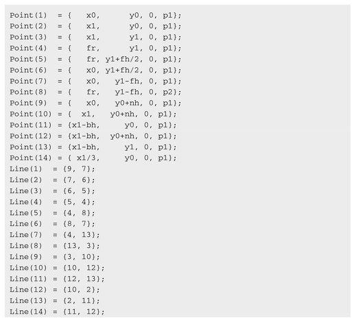
Next, boundary conditions and subdomains are marked:

We generate a 2D mesh for the domain and save it in the file mesh.msh. Then we convert the generated mesh into the xml-format:

The numerical algorithm is implemented in the FEniCS framework. The problem statement is described in the ufl-file, where we define linear and bilinear forms:

The above ufl-file includes definitions of three bilinear and three linear forms for evaluating temperature and electric potential as well as for the visualization of the influence of the electric potential on heat.

We generate the header file Joule. h from the ufl-file in order to import it into the main source code:

It is also necessary to include the dolfin.h library in addition to the header file Joule.h:

Listing 11.41.

We create an object for the computational mesh taken from the file mesh. xml, an object with marks for computational domain boundaries and an object including marks for subdomains Ω₁ and Ω₂:

Listing 11.42.

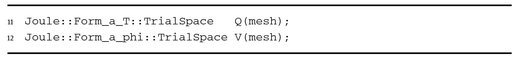
Next, we introduce spaces for the temperature and electric potential:

Listing 11.43.

We also create functions T and phi for the required solution, and the function for storing temperature values corresponding to the previous time level:

Listing 11.44.

Further, we define constants for the time step, environment temperature, and equation coefficients:

Listing 11.45.

It is also necessary to create Dirichlet boundary conditions for the electric potential. The appropriate space, boundary value, and object with boundary marks are specified in the parameters:

Listing 11.46.

Now we define the initial temperature distribution:

Listing 11.47.

Next, we create objects for bilinear and linear forms. We must introduce the appropriate functions or constants for each object from the forms:

Listing 11.48.

Further, we create objects for matrices and vectors for evaluating mesh functions, specify linear solvers (gmres is applied as the iterative solver for both searching variables):

Listing 11.49.

The values from each time level are saved as files in the vtk format for post-processing of the results, and can be visualized by ParaView:

Listing 11.50.

Time-integration is carried out with a uniform time step. We display the current step on the screen:

Listing 11.51.

Then matrices and vectors are assembled, boundary conditions are applied, and temperature and electric potential are evaluated at the new time level:

Listing 11.52.

Results for the current time level are saved into the files:

Listing 11.53.

At the end of the time step calculations, the values from the current time level are assigned to the objects storing the previous time level values:

Listing 11.54.

We compute the auxiliary function f = σ| grad φ|² to visualize the released heat:

Listing 11.55.

11.4.4 Numerical simulations

The numerical results obtained for the above problem are presented below. Computations were carried out on the grid with 7,845 triangular cells shown in Figure 11.20 with the time step equalling τ = 1 minute up to the final time T_max = 60 minute. On boundary Γ₁, the Dirichlet boundary condition φ = 1 is imposed for the electric potential, and on boundary Γ₆, the potential value is treated as zero. Robin boundary conditions are specified on boundaries Γ₁, Γ₂, and Γ₄ for the temperature, where heat exchange from iron to the environment with the temperature T_air = 22.0 is imposed. Heat exchange with a lower coefficient of convective heat transfer is given on boundary Γ₃.

Computational results for temperature, electrical potential and function f are depicted in Figures 11.21, 11.23 and 11.24, respectively. Figure 11.22 shows the time-histories for the maximal and minimal temperatures which illustrate the evolution of the temperature to a quasi-stationary state.

Fig. 11.20. Computational grid.

Fig. 11.21. Temperature distribution after 1, 2 and 3 hours (from left to right).

Fig. 11.22. Maximal and minimal temperature time-histories.

Fig. 11.23. Electric potential distribution after 3 hours.

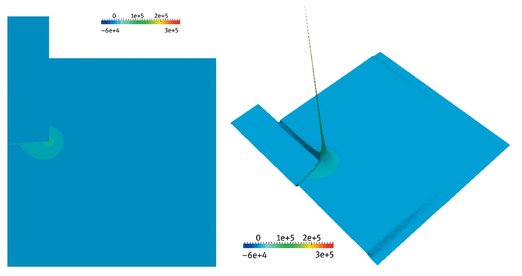
Fig. 11.24. Distribution of the f = σ| grad φ|² function.