5 ParaView: An efficient toolkit for visualizing large datasets
Abstract: In this chapter, we consider a portable open source software package for visualizing scientific datasets: ParaView10. Basic data formats used in the program are described below. We also discuss the preparation of input data on the basis of simple examples. Finally, the feature of parallel visualization is demonstrated.
5.1 An overview
We can download ParaView installation files from the official website (for Windows, Linux, and Mac). Here the focus is on the Ubuntu version. To install the application, we use the following command:
ParaView allows visualization of scientific datasets, both on local computers and on parallel computing systems. The program has client-server architecture; it was developed on the basis of the visualization ToolKit (VTK) library11. It is possible to work with ParaView via the graphical user interface (GUI) or in batch mode using the Python programming language. The visualizer supports standard features of scientific visualization with the focus on two- and three-dimensional data. Other products, such as Tecplot12, visIt13, and Ensight14 can be considered analogs.
ParaView supports datasets defined on uniform and non-uniform, rectilinear and curvilinear, general non-structured and multiblock grids. The VTK format is the basic data format. ParaView can also import a large number of other data formats, i.e.,STL15, NetCDF16, CAS17 and more.
ParaView provides a large set of useful filters for data analysis. Users can also create their own filters. The program allows visualization of scalar and vector fields. Using filters, we can extract contours and isosurfaces, intersect domains with a plane or a given function, conduct data analysis, display streamlines for vector fields, and plot distribution of data values over given lines. We can also save screenshots and animation for time-dependent fields.
5.2 Data file formats
The VTK format has two different styles of data presentation: serial and XML based formats. The serial formats are text files, which can be easily written and read. The XML based formats support random access and parallel input/output. These formats also provide better data compression.
5.2.1 Serial formats
The serial formats consist of the following five basic parts:
- – The file version and identifier. This part contains the single line: #vtk Datafile Versionx.x.
- – The header consists of a string with at the end. The maximum number of characters is 256. The header can be used to describe the dataset and includes any other information.
- – The file format which indicates the type of file; files may be in the (ASCII ) code or binary (BINARY).
- – The structure of the dataset which describes its geometry and topology. This part begins with the keyword DATASET followed by the type of dataset. Other combinations of keywords and data are then defined.
- – The attributes of the dataset which begin with the keywords POINT_DATA or CELL_DATA, followed by the number of points or cells, respectively. Other combinations of keywords and data define the dataset attribute values such as scalars, vectors, tensors, normals, texture coordinates, or field data.
This structure of serial files provides freedom to select dataset and geometry and to change data files using filters of VTK or other tools.
VTK supports five different dataset formats: structured points, structured grid, rectilinear grid, unstructured grid, and polygonal representation.
5.2.1.1 Structured points
This file format allows storage of a structured point dataset. Grids are defined by the dimensions nx, ny, nz, the coordinates of the origin point x, y, z, and the data spacing sx, sy, sz.

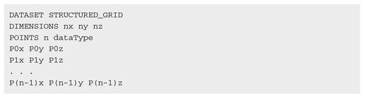
5.2.1.2 Structured grid
This file format allows storage of a structured grid dataset. Grids are described by the dimensions nx, ny, nz and the number of points, n. The POINT section consists of the coordinates of each point.
5.2.1.3 Rectilinear grid
This file format is oriented to store a rectilinear grid dataset. Grids are defined by the dimensions nx, ny, nz, and three lists of coordinate values.

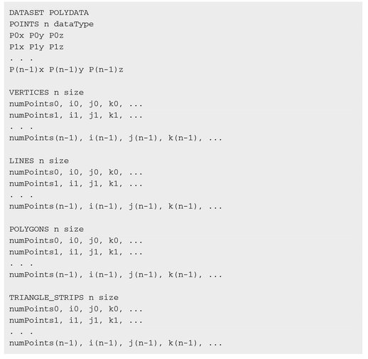
5.2.1.4 Polygonal representation
This format provides storage of an unstructured grid dataset and consists of arbitrary combinations of primitives (surfaces, lines, points, polygons, triangle strips). Grids are described by POINTS, VERTICES, LINES, POLYGONS, TRIANGLE_STRIPS. Note that here POINTS is the same as the POINTS in structured grid.
5.2.1.5 Unstructured grid
This format is designed for storing unstructured grid datasets. An unstructured grid is defined by vertices and cells. The CELLS keyword requires two parameters: the number of cells n, and the size of the cell list size. The cell list size indicates the total number of integer values required to represent cells. The CELL_TYPES keyword requires the only parameter, i.e. the number of cells n that should be equal to the value in CELLS. The cell types data are integer values specifying the type of each cell.

5.2.2 XML formats
Data formats based on XML syntax provide many more features. The main feature is data streaming and parallel input/output. These data formats also provide data compression, random access, multiple file representation of data, and new file extensions for different VTK dataset types.
There are two different types of XML formats:
- – the serial type is applied to read and write employing a single process;
- – the parallel type is applied to read and write using multiple processes. Each process writes or reads only its own part of data which is stored in an individual file.
In the XML format, datasets are divided into two categories: structured and unstructured categories.
A structured dataset is a regular grid. The structured dataset types are vtkImage Data, vtkRectilinearGrid, and vtkStructuredGrid.
An unstructured dataset defines an irregular grid that is a set of points and cells. The unstructured dataset types are vtkPolyData or vtkUnstructuredGrid.
XML formats are designed similarly to serial formats. A more detailed description can be found in the ParaView documentation.
5.3 Preparing data
Let us consider simple examples of how to prepare data using the given data visualization formats. We present the implementation of writing the results of mathematical modeling in a file.
5.3.1 Structured 2D grid
Using the above description of the serial data representation format, we write values of a two-dimensional grid function in a VTK file. We use the following function to generate the grid dataset:
Function values are calculated on the uniform rectangular grid 100 x 100.
Consider the implementation of the program. First, to work with mathematical functions and to write to a file, we include the standard libraries as shown in Listing 5.1.
Listing 5.1.

Further, we set the dimensions of the grid as follows:
Listing 5.2.

Define the function to calculate a 2D structured dataset as shown Listing 5.3.
Listing 5.3.

Next, we set the function which writes the dataset to a file with VTK serial format as follows in Listing 5.4.
Listing 5.4.
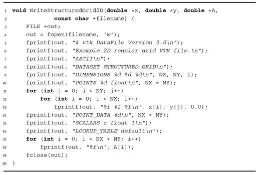
In the main function, it is necessary to specify domain parameters, generate the coordinates vectors x, y, calculate values of the function v, and write into a file as shown in Listing 5.5 below.
Listing 5.5.


Fig. 5.1. Structured 2D grid dataset.
Finally, we visualize the resulting file vtk2d.vtk using ParaView as shown in Figure 5.1.
5.3.2 Structured 3D grid
Here we present an example of generating a structured 3D grid dataset and writing it to a VTK file.
The dataset corresponds to the following function:
with the regular uniform grid 100 x 100 x 50.
The complete code of the program is shown in Listing 5.6 below; the implementation is the same as in the 2D example.
Listing 5.6.


We visualize the resulting file vtk3d.vtk via ParaView (Figure 5.2).

Fig. 5.2. The surface of the 3D dataset.
5.3.3 Unstructured 2D grid
In the case of unstructured 2D grids, it is reasonable to employ special software. Of course, we can use the VTK library itself, but there are other libraries which are more convenient for writing VTK files.
Let us consider the visIt library18, and in particular the visit_writer module. This module provides a convenient interface for writing VTK files and allows the writing of unstructured grids.
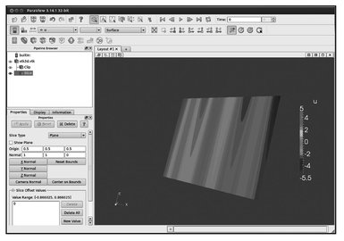
Fig. 5.3. Slice.
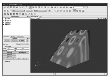
Fig. 5.4. Clip.
visit_writerincludestwofiles(visit_writer.candvisit_writer.h).The following code (Listing 5.7) writes an unstructured grid dataset to a VTK file using the library.
Listing 5.7.

We visualize the resulting file unsctructured2d. vtk using ParaView as demonstrated in Figures 5.3 and 5.4. It is possible to visualize the data associated with the nodes (Figure 5.5) and cells (Figure 5.6).

Fig. 5.5. Nodal data.
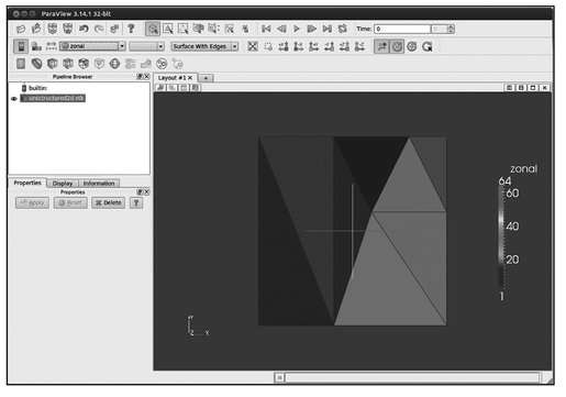
Fig. 5.6. Cell data.
5.4 Working with ParaView
The user interface of ParaView consists of the following sections:
- – Toolbars provides quick access to frequently used functions;
- – Pipeline Browser displays a list of objects (opened files and the filters applied to them) and allows selection of the objects for visualization;
- – Object Inspector contains three tabs:
- – the Properties tab provides options to change properties of selected objects;
- – the Display tab provides access to parameters of selected objects;
- – the Information tab provides basic statistics on objects.
- – View area displays objects.
5.4.1 Loading data
The File | open command or the Open button from the toolbar can be used to load data into ParaView. It is necessary to select a file, for example file vtk2d.vtk from the previous section (Figure 5.7). Next, we click the Apply button in Object Inspector (the Properties tab). If a data file contains more than one function for visualization, then the same color will be used over an entire dataset (solid Color).

Fig. 5.7. Loading data.
In this case, we select a function in the Toolbars or the Display tab of object Inspector. Then the dataset will be colored based on the values of the function. The color palette of the function may be edited from the dialog that appears from clicking the Edit Color Map button.
5.4.2 Filters
After a file is loaded, we can use the mouse buttons to zoom, pan, rotate or roll an object. For a more detailed study of the object, filters for processing data should be applied. The most common filters are listed in Table 5.1. The results of applied filters are displayed in Pipeline browser.
Table 5.1. Common filters.
| Filter | Description |
|---|---|
| Evaluates a user-defined expression on a per-point or per-cell basis. | |
| Extracts the points, curves, or surfaces where a scalar field is equal to a user-defined value. | |
| Intersects an object with a half-space. | |
| Intersects an object with a plane. | |
| Extracts cells that lie within a user-defined range of a scalar field. | |
| Extracts a subset by defining either a volume of interest or a sampling rate. | |
| Places a glyph on each point in a mesh. | |
| Seeds a vector field with points and then traces those points through the (steady state) vector field. | |
| Displaces each point in a mesh by a given vector field. | |
| Combines the output of several objects into a dataset. | |
| Extracts one or more items from a dataset. |
These filters are only a small example of the possibilities available. Currently, ParaView offers more than one hundred. For convenience, the Filters menu is divided into submenus (Table 5.2).
The use of filters to process and visualize generated 3D structured dataset is now demonstrated (file vtk3 d. vtk):
- – load and display the dataset u from the file vtk3 d. vtk (Figure 5.8);
- – apply the slice filter. (The parameters of the filter are set before applying the filter; see Figure 5.9);
- – similarly, build part of the object using the Clip filter (Figure 5.10);
- – apply the Contour filter. (The contour values are specified in the Properties tab of Object Inspector; see Figure 5.11).
Table 5.2. Filters menu.
| Submenu | Description |
|---|---|
| Search | Searches through lists of filters |
| Recent | Recently used filters |
| Common | Common filters |
| Cosmology | Filters developed at LANL for cosmology research |
| Data Analysis | Filters designed to obtain quantitative values |
| Statistics | Filters which provide descriptive statistics of data |
| Temporal | Filters which analyze or modify data that changes over time |
| Alphabetical | Alphabetical list of filters |
In addition, we can display the color legend of an object by clicking the button ![]() . Clicking the button
. Clicking the button ![]() , we edit the color map (palette) as well as the number of colors in the color map (Resolution slider). To save screenshots, the File | save Screenshot menu command is available.
, we edit the color map (palette) as well as the number of colors in the color map (Resolution slider). To save screenshots, the File | save Screenshot menu command is available.

Fig. 5.8. Step 1.
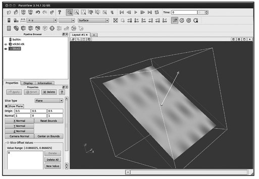
Fig. 5.9. Step 2.
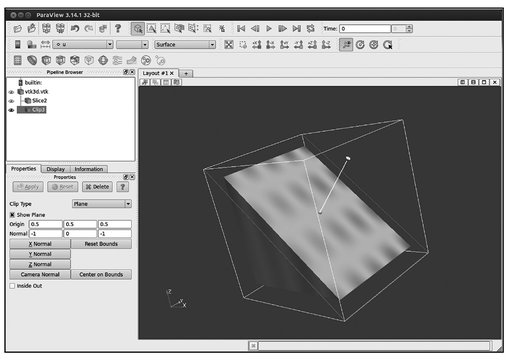
Fig. 5.10. Step 3.

Fig. 5.11. Step 4.
5.4.3 Time series
In order to work with transient fields, we need to create a pvd file which contains information about the time steps and files with data of this time step:

Each individual file can contain a grid of any type: vtu = unstructured, vtp = polydata, vtr = rectilinear, vti = imagedata. At the same time, the file can be binary, text, compressed or not compressed.
We can play a time-history with the VCR control toolbar. In addition, it is possible to save the current time series as an animation using the File | save Animation menu command.
5.5 Parallel visualization
ParaView provides the possibility of parallel visualization and data processing to work with large datasets. We now briefly describe the architecture of ParaView to help understand this parallelism.
5.5.1 The architecture of ParaView
ParaView has a three-level client-server architecture and consists of the following parts:
- – Data Server is responsible for reading, processing and writing data. All objects in Pipeline Browser are located on Data Server. It may in turn be parallel.
- – Render Server is responsible for rendering data and can be parallel.
- – client is responsible for displaying data. The client controls the creation of objects, their implementation, and deletion from servers, but does not contain data itself. The user interface is part of the client. The client is a serial program.
These parts of the program may be located on different computing systems, but they are often integrated into a single application. There are three modes of starting ParaView:
- – The standard mode, when all three parts are combined in one application.
- – The Client/Server mode, when Data Server and Render Server act as the server to which the client connects. In this case, we use the pvserver command, which runs the data and render servers.
- – The Render/server mode, when all three parts are run as separate applications. This mode is suitable for work with very large data. The client connects to the Render server, which is in turn connected with the Data server. The Render/server mode should only be used in special cases. For example, the power of a parallel system is not enough for both servers and they must be separated.
5.5.2 Running in parallel mode
Modern computers are parallel computing systems and can provide significant performance improvement due to multiprocessor architecture. Here we consider running ParaView in the Client/Server mode. To do this, we run the server using the following command:
This command runs the parallel server in four processes.
Further actions are associated with connecting the client to the parallel server. We invoke ParaView and click on the Connect button. Next, in the opened dialog, we click on the button Add server and set the name or ip address. Finally, we can open files as usual, for instance, the file vtk3 d. vtk as presented in Figure 5.12.

Fig. 5.12. Opening the file on the parallel server.
After applying the filter Process Id Scalars, we can choose the array ProcessId to display subdomains belonging to different processes (Figure 5.13).

Fig. 5.13. Process Id Scalars.