9 PETSc for parallel solving of linear and nonlinear equations
Abstract: The Portable, Extensible Toolkit for Scientific Computation (PETSc)39 is a set of data structures and routines used to implement large-scale scientific computations on parallel (and serial) computers. Only the basic features of PETSc and its solvers are discussed here.
9.1 Preliminaries
In this section, we consider the main possibilities of PETSc, its installation, and development of programs under this platform.
9.1.1 Brief description
PETSc provides a large set of tools for the numerical solution of partial differential equations on high-performance computers. It facilitates the development of large-scale applications in Fortran, C / C++, and Python programming languages. PETSc supports MPI40, shared memory threads, and GPUs through CUDA or OpenCL, as well as hybrid MPI-shared memory threads or the MPI-GPU parallelism.
PETSc consists of a variety of modules (similar to classes in c++). Each module employs a particular family of objects (e.g. vectors) and provides basic operations for working with them. The basic modules of the library are the following:
- – Index sets (IS) are objects for indexing into vectors, matrices, renumbering, etc.;
- – Vectors (Vec);
- – Matrices (Mat);
- – Data management (DM), for managing interactions between mesh data structures, vectors and matrices;
- – Krylov subspace methods (KSP);
- – Preconditioners (PC);
- – Scalable nonlinear equations solvers (SNES);
- – Time-steppers (TS) for solving time-dependent PDEs.
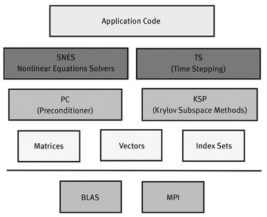
Fig. 9.1. Organization of the PETSc modules.
Figure 9.1 presents a diagram of the PETSc modules illustrating the hierarchical organization of this platform.
A structure like this allows users to employ the most appropriate abstraction level for a particular problem.
9.1.2 Installation
It is easy enough to download the source code of PETSc from the official website41 and to install it according to the instructions42.
To install the library on the Ubuntu operating system, the following command must be performed:
To build programs in c with PETSc, we use
For programs in c++, we apply the following command:
Note that we consider compiling programs on the Ubuntu operating system.
To run a program, we employ the following command:
np is the number of processes.
9.1.3 Development of programs
Header files containing the procedures necessary for the use of PETSc components (modules) must be specified in order to write PETSc-based applications.
where includefile.h maybe as follows:
- – petsc.h - for basic PETSc procedures;
- – petscvec.h - to deal with vectors;
- – petscmat.h - to work with matrices;
- – petscpc.h - for preconditioners;
- – petscksp.h - for the linear solver library;
- – petscsys . h - for PETSc system procedures;
- – petscviewer.h-for viewers.
An included header file must correspond to the highest level of PETSc objects used in a program. All required lower level header files will be included automatically in the higher level files.
All PETSc programs begin with the function below.
This function initializes PETSc and MPI. The arguments argc and argv are command line arguments used in all C/C++programs. The file argument sets the name of a PETSc options file, the help argument is a character string which will be printed if the program is executed with the –help option. The last two arguments are optional.
Petsc Initialize sets the PETSc world communicator named PETSC_COMM_ WORLD by default. Communicators are variables of the MPI_Comm type. In most cases, we can apply the PETSC_COMM_WORLD communicator to show all processes launched. The PETSC_COMM_SELF communicator is used to show a single process.
PetscFinalize must be called at the end of the program. This calls MPI_ Finalize, if PetscInitialize ran MPI. Between PetscInitialize and PetscFinalize, a code with PETSc objects and solvers suitable for a particular problem is written.
9.1.4 Matrices and vectors
It is not necessary to program the basic data exchange directly through MPI in order to exploit PETSc. Many message passing details in PETSc are invisible in such objects as vectors and matrices. In addition, PETSc provides tools such as generalized vector distribution/assembly and distributed arrays to control parallel data. Users should still know the basic concepts of message passing and be able to work with distributed memory, however.
An example of working with vectors and matrices, where the matrix-vector multiplication is calculated is:
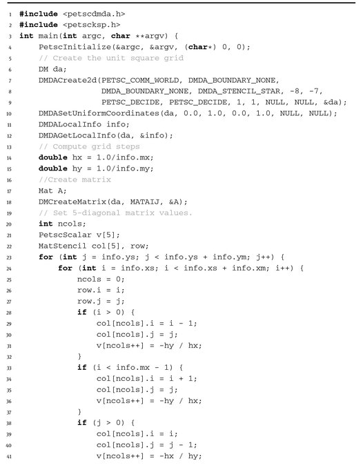
Since a discrete (grid) problem is formulated to solve PDEs numerically, we now consider a matrix and vector defined on a structured grid in Listing 9.1.
Listing 9.1.


The header file petscdmda.h is included at the beginning of the program by using the command in Listing 9.2.
Listing 9.2.
To initialize PETSc and MPI, see Listing 9.3 below.
Listing 9.3.
The da object is then created, which is used to manage parallel communications because it contains information about the grid and its distribution by processes.
Listing 9.4.

Here the domain is the unit square.
Usually, each processor requires its local part of the vector x with ghost points (the boundaries of vectors in the neighboring processors) to estimate the local function f (x). The ghost points of a two-dimensional regular mesh distributed over processes are shown in Figure 9.2. Each rectangle belongs to a separate process.

Fig. 9.2. Ghost points.
In order to create the da structure, we set the communicator, types of the array periodicity, xperiod and yperiod, the type of stencil (DMDA_STENCIL_STAR for the five-point stencil or DMDA_STENCIL_BOX for the nine-point stencil), the dimension of the grid in each direction (it can also be set from the command line via the da_grid_x, da_grid _y N), and other parameters. We can also create DM objects to control one-dimensional or three-dimensional data.
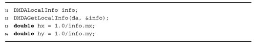
Information about the mesh is contained in the DMDALocalInfo structure, which can be obtained using the DMDAGetLocalInfo command below in Listing 9.5.
Listing 9.5.
Next, we create the matrix as shown in Listing 9.6.
Listing 9.6.

da is the DM object and MATAIJ is the type of matrix. The MATAIJ type corresponds to sparse matrices.
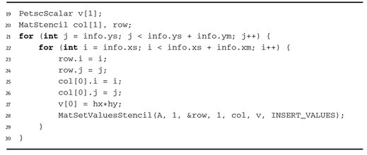
For simplicity, we consider the diagonal matrix. Its values can be specified with the following commands (Listing 9.7):
Listing 9.7.
After all values have been inserted into the matrix, it must be assembled with the pair of commands shown below in Listing 9.8.
Listing 9.8.

Then we create the global and local vectors as follows in Listing 9.9.
Listing 9.9.

We set values of vector equal to one in Listing 9.10.
Listing 9.10.
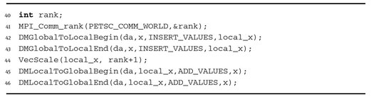
We then modify the values of the vector x according to the rank of a running process. To do this, we obtain the local vector from the global vector and modify its values, and then conduct the inverse operation to obtain the global vector from the local one; see Listing 9.11.
Listing 9.11.
To calculate the matrix-vector product, we create vector y as follows:
Listing 9.12.

The product is then computed as shown below in Listing 9.13.
Listing 9.13.
The most common vector and matrices operations are presented in Tables 9.1 and 9.2, respectively.
We write the vectors x and y to files as follows in Listing 9.14.
Listing 9.14.

To write data to a file, we use the function shown below in Listing 9.15.
Listing 9.15.

This results in output of a vector to a VTK file using the PetscViewer structure. Here we employ ParaView for visualizing files.
Finally, we must destroy all objects as follows in Listing 9.16.
Listing 9.16.

The PetscFinalize function is then called.
Table 9.1. Basic vector operations of PETSc.
| Function | Operation |
|---|---|
| VecAXPY(Vec y, PetscScalar a, Vec x); | y = y + a * x |
| VecAYPX(Vec y, PetscScalar a,Vec x); | y = x + a * y |
| VecWAXPY(Vec w, PetscScalar a,Vec x, Vec y); | w = a ∗ x + y |
| VecAXPBY(Vec y, PetscScalar a, PetscScalar b, Vec x); | y = a ∗ x + b ∗ y |
| VecScale(Vec x, PetscScalar a); | x = a ∗ x |
| VecDot(Vec x, Vec y, PetscScalar *r); | |
| VecTDot(Vec x, Vec y, PetscScalar *r); | r = x‘ * y |
| VecNorm(Vec x,NormType type, PetscReal *r); | r = ||x||type |
| VecSum(Vec x, PetscScalar *r); | r = ∑xj, |
| VecCopy(Vec x, Vec y); | y = x |
| VecSwap(Vec x, Vec y); | y = x while x = y |
| VecPointwiseMult(Vec w, Vec x, Vec y); | wj = xj * yj |
| VecPointwiseDivide(Vec w, Vec x, Vec y); | wj = xj/yj |
| VecMDot(Vec x, int n,Vec x, Vec y[], PetscScalar *r); | |
| VecMTDot(Vec x, int n,Vec y[], PetscScalar *r); | r[j] = x’ * y[i] |
| VecMAXPY(Vec y, int n, PetscScalar *a, Vec x[]); | y = y + ∑jaj * x[j] |
| VecMax(Vec x, int *idx, PetscReal *r); | r = max xj |
| VecMin(Vec x, int *idx, PetscReal *r); | r = min xi |
| VecAbs(Vec x); | xj = |xj| |
| VecReciprocal(Vecx); | xj = 1/xj |
| VecShift(Vec x, PetscScalar s); | xj = s + xj |
| VecSet(Vec x, PetscScalar alpha); | xj = α |
Table 9.2. Basic matrices operations of PETSc.
| Function | Operation |
|---|---|
| MatAXPY(Mat Y, PetscScalar a, Mat X, MatStructure str); | Y = Y + a ∗ X |
| MatMult(Mat A,Vec x, Vec y); | y = A * x |
| MatMultAdd(Mat A,Vec x, Vec y,Vec z); | z = y + A ∗ x |
| MatMultTranspose(Mat A,Vec x, Vec y); | y = AT * x |
| MatMultTransposeAdd(Mat A,Vec x, Vec y, Vec z); | z = y + AT * x |
| MatNorm(Mat A,NormType type, double *r); | r = ∥A∥type |
| MatDiagonalScale(Mat A, Vec 1,Vec r); | A = diag(l) ∗ A ∗ diag(r) |
| MatScale(Mat A,PetscScalar a); | A = a * A |
| MatConvert(Mat A,MatType type,Mat *B); | B = A |
| MatCopy(Mat A,Mat B,MatStructure); | B = A |
| MatGetDiagonal(Mat A,Vec x); | x = diag(A) |
| MatTranspose(Mat A, MatReuse, Mat* B); | B = AT |
| MatZeroEntries(MatA); | A = 0 |
| MatShift(Mat Y, PetscScalar a); | Y = Y + a * I |
For instance, we compile and run the program on 8 parallel processes as shown below:
Figure 9.3 demonstrates the calculated vector y. It should be noted that all PETSc functions return an integer value which indicates the presence or absence of an error during the call. The macro CHKERRQ (ierr) checks the value of ierr and invokes the error handler if an error occurs. CHKERRQ (ierr) is recommended in all procedures to determine a complete list of errors.

Fig. 9.3. The vector y, Y = Ax.
Thus, PETSc offers effective codes for the various phases of solution with a unified approach for each class of problems. This design ensures easy use and comparison of different algorithms, as well as easy configuration and expansion. PETSc provides a set of mechanisms (the support of Nvidia for graphics devices, use of complex numbers in applications, visualization tools, debugging, profiling, etc.) required for writing parallel applications.
9.2 Solvers for systems of linear equations
We now consider an example of solving a model boundary value problem using the KSP module. An initial differential problem is reduced to a system of linear algebraic equations by applying the finite difference method. The Krylov subspace iterative method is used to solve the system of equations.
9.2.1 Problem formulation
We consider the Poisson equation
with homogeneous Dirichlet boundary conditions
(9.2)
The function u(x), x = (x1, x2) is defined in the domain
For simplicity, we put
(9.3)
We need to find an approximate solution of equations (9.1)–(9.3).
9.2.2 Finite difference approximation
We introduce a uniform grid with steps h1 (Mh1 = 1) and h2 (Nh2 = 1) in the corresponding direction and apply the finite difference approximation in space for the problem (9.1)–(9.3). We obtain the following grid problem in the form of the system of linear algebraic equations with the unknown vector yij, i = 0, 1, ... , M, j = 0, 1, ... , N:

(9.4)
(9.5)
The difference solution is determined at internal nodes of the grid.
The system can be written in the form of a matrix problem:
where y = yij is the unknown vector, A = aij is the coefficient matrix, and b is the vector on the right. The matrix of this system has a diagonal structure and is sparse (only five diagonals contain non-zero values). It seems reasonable to employ an iterative method to solve the system.
9.2.3 Numerical implementation
The parallel implementation of the numerical solution of the considered problem via the KSP module is presented in Listing 9.17 below.
Listing 9.17.

First, the header files are included. The “petscdmda.h” file allows the use of distributed arrays DMDA. The “petscksp.h” file is necessary to employ KSP solvers as follows:
Listing 9.18.

Listing 9.19 shows how to initialize PETSc and MPI.
Listing 9.19.
The da object is then created. The 2D structured uniform grid for the unit square is built and information about it obtained as shown below in Listing 9.20.
Listing 9.20.

In order to solve the problem it is necessary to form the matrix and the vector on the right. The parallel matrix for the da object is created as follows in Listing 9.21.
Listing 9.21.
The MATAIJ type corresponds to a sparse matrix. The result is an empty matrix A.
Next, the five-diagonal coefficient matrix is filled according to finite difference approximation (9.4).
Listing 9.22.


Then the vector of the approximate solution x and the vector on the right b is created as shown in Listing 9.23.
Listing 9.23.

We set the values of the vector b as follows:
Listing 9.24.
After designing the matrix and vectors, the linear system Ax = b is solved using the KSP object. First, the KSP object is created as shown in Listing 9.25.
Listing 9.25.
Then, we define the operators associated with the system as shown below:
Listing 9.26.
The matrix A serves as a preconditioning matrix in this case. The parameter DIFFERENT_ NONZERO_PATTERN is a flag which gives information about the structure of the preconditioner.
To specify various options of the solver, we apply the command shown in Listing 9.27.
Listing 9.27.
This command allows users to customize the linear solver by a set of options at runtime. Using these options, we can specify an iterative method and the type of preconditioners, determine the stability and convergence, as well as set various monitoring procedures.
To solve the linear system, see Listing 9.28 below.
Listing 9.28.
b and x are the vector on the right and unknown vector, respectively. KSP uses the GMRES method with the ILU preconditioner in the case of sequential run and block Jacobi in the case of parallel running by default.
The desired method for solving systems of linear equations is defined by the following command which specifies the method:
Table 9.3 presents a list of available methods.
Table 9.3. Methods for solving systems of linear equations.
| Method | KSPType | Option name |
|---|---|---|
| Richardson | KSPRICHARDSON | richardson |
| Chebychev | KSPCHEBYCHEV | chebychev |
| Conjugate Gradient | KSPCG | cg |
| BiConjugate Gradient | KSPBICG | bicg |
| Generalized Minimal Residual | KSPGMRES | gmres |
| BiCGSTAB | KSPBCGS | bcgs |
| Conjugate Gradient Squared | KSPCGS | cgs |
| Transpose-Free Quasi-Minimal Residual (1) | KSPTFQMR | tfqmr |
| Transpose-Free Quasi-Minimal Residual (2) | KSPTCQMR | tcqmr |
| Conjugate Residual | KSPCR | cr |
| Least Squares Method | KSPLSQR | lsqr |
| Shell for no KSP method | KSPPREONLY | preonly |
A method for solving the system of equations can also be set by the command line option -ksp_type, values of which are listed in the third column of Table 9.3.
Next, we get the number of iterations its and print it as follows:
Listing 9.29.
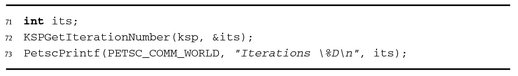
The its parameter provides either the number of iterations used until convergence is reached or the number of iterations performed until discovery of divergence or interruption.
Finally, all objects are destroyed as shown in Listing 9.30.
Listing 9.30.

In the example below we compile and run the program on 4 parallel processes.
The result is
Figure 9.4 shows the solution of the problem.

Fig. 9.4. The solution of the Dirichlet problem for the Poisson equation.
9.3 Solution of nonlinear equations and systems
Most of the problems requiring solutions of differential equations are nonlinear. PETSc offers the SNES module for the solution of nonlinear problems.
Built on the basis of KSP linear solvers and PETSc data structures, SNES provides an interface to use Newton’s method and its various modifications.
An example of solving a nonlinear problem using the SNES module follows.
9.3.1 Statement of the problem
we consider the nonlinear equation
(9.6)
with the boundary conditions

(9.7)
For our problem, we define q(u) as
9.3.2 Solution algorithm
Newton’s method is in common use for the solution of nonlinear problems of mathematical physics:
(9.8)
Newton’s method has the following general form:
(9.9)
where J(uk) = F′(uk) is the Jacobian and u0 is the initial approximate solution.
In practice, Newton’s method (9.9) is realized in two steps:
- – Solve (approximately): J(uk)δuk = –F(uk).
- – Update: uk+1 = uk + δuk.
We apply this method to solve the problems (9.6), (9.7). Assume that δ uk is sufficiently small, then the problem can be linearized with respect to δ uk. Now the nonlinear coefficient q(u) is linearized:
(9.10)
Treating δ uk as an unknown, we obtain the equation
(9.11)
Collecting elements for the unknowns δ uk on the left, we obtain the system of linear equations
(9.12)
The system can be represented in the matrix form
from which δ uk is determined. Using the calculated δ uk, we find uk+1 = uk + δuk.
The basic computational complexity of Newton’s method is associated with the need to solve a linear system of equations.
9.3.3 Implementation in PETSc
The parallel implementation of the solution of the nonlinear problem using Newton’s method is given in Listing 9.31 below.
Listing 9.31.

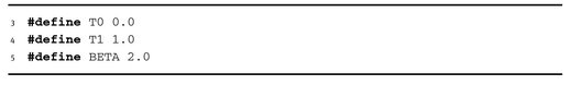
The parameters for the function q(u) = uβ and boundary conditions are specified as shown in Listing 9.32.
Listing 9.32.
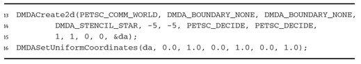
Next, the da object is created as follows in Listing 9.33.
Listing 9.33.
For the numerical solution, we invoke the nonlinear solver as shown in Listing 9.34.
Listing 9.34.

To initialize it, the functions F and J should be set as follows:
Listing 9.35.

The function for the initial approximation is needed as shown below in Listing 9.36.
Listing 9.36.
T1 = 1.0 is set as the initial guess as follows:
Listing 9.37.

The function used for setting F is shown below in Listing 9.38.
Listing 9.38.
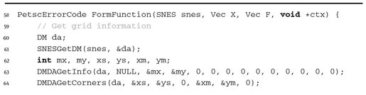


Here we use the finite difference approximation on the five-point stencil with the boundary conditions.
The function for the calculation J is given directly in Listing 9.39.
Listing 9.39.


To compute the Jacobian, we use the explicit expression.
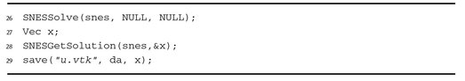
For the numerical solution of the nonlinear system, the function SNESSolve is called and the solution saved as shown in Listing 9.40 below.
Listing 9.40.
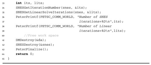
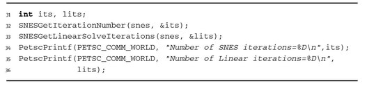
We then obtain the number of linear and nonlinear iterations and print it as shown in Listing 9.41 below.
Listing 9.41.
Finally, the work space is freed as follows:
Listing 9.42.

and PetscFinalize called.
In this example, we compile and run the program on 4 parallel processes as follows:
The result is

The solution of the problem is depicted in Figure 9.5.

Fig. 9.5. The solution of the nonlinear problem.
9.4 Solving unsteady problems
PETSc provides the TS module to solve unsteady PDEs. TS employs SNES to solve nonlinear problems at each time level.
9.4.1 Problem formulation
In the rectangle
we consider the unsteady equation
(9.13)
supplemented with the boundary conditions
(9.14)
For the unique solvability of the unsteady problem, we set the initial condition
(9.15)
where c = const, r = ((x1 – 0.5)2 + (x2 – 0.5)2)1/2, x ∊ Ω.
9.4.2 Approximation
The scheme with weights is applied to solve this transient problem after approximation in space.
For simplicity, we define the following uniform grid in time:
and in space:
where ω is the set of interior nodes and ∂ω is the set of boundary nodes.
We write the two-level scheme with weights for the problems (9.13)–(9.15) as follows:
(9.16)
(9.17)
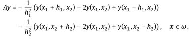
The discrete operator A is defined as
If ϭ = 0, we have the explicit scheme, whereas for ϭ = 1, the scheme is implicit.
9.4.3 The program
The program for the numerical solution of the time-dependent problem using the module TS is shown in Listing 9.43 below.
Listing 9.43.


Unlike the previous examples, the TS solver is used as follows:
Listing 9.44.

The TS module is intended to solve ordinary differential equations (ODEs) written as
which are obtained after the discretization of unsteady problems in space. The module provides solvers which use the forward and backward Euler methods. We can also solve the stationary equations
and differential-algebraic equations
The solution method is preset using the command
Listing 9.45.
where TSPSEUDO is the method with pseudo time-stepping. Instead of this method, we can use
- – TSEULER - the solver involving the forward Euler method;
- – TSSUNDIALS - the solver based on the package SUNDIALS;
- – TSBEULER - the backward Euler method.
Since TS is implemented on the basis of the nonlinear solver SNES, it should be handled via SNES. We must set the Jacobian, the vector on the right, and the initial approximation as shown below in Listing 9.46.
Listing 9.46.

The Jacobian is defined by the following functions according to the problem statement:
Listing 9.47.


The function to set the initial approximation is shown in Listing 9.48.
Listing 9.48.


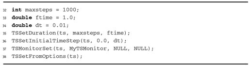
Then time parameters are set as shown in Listing 9.49 below.
Listing 9.49.
The function MyTSMonitor allows the result to be written into a file at each time level as follows in Listing 9.50.
Listing 9.50.

Next, the procedure for solving an unsteady problem is called as illustrated in Listing 9.51.
Listing 9.51.
Using the following commands, we obtain and print the number of completed time steps as follows:
Listing 9.52.

We compile and run the program on 4 parallel processes:
The output is

Figure 9.6 shows the solution of the problem at the final time level.

Fig. 9.6. The solution of the unsteady problem.