
4 MPI technology
Abstract: Message Passing Interface Standard (MPI)1 is a portable, efficient, and flexible message-passing standard for developing parallel programs. Standardization of MPI is performed by the MPI Forum, which incorporates more than 40 organizations including suppliers, researchers, software developers, and users. MPI is not, however, an IEEE or ISO standard but, in fact, an industry standard for writing message-passing programs for high-performance computing systems. There are a large number of MPI implementations, including both commercial and free variants. MPI is widely used to develop programs for clusters and supercomputers. MPI is mainly oriented to systems with distributed memory where the costs of message-passing are high, while OpenMP is more appropriate for systems with shared memory (multicore processors with shared cache). Both technologies can be applied together in order to optimally employ multicore systems.
4.1 Preliminaries
Here the basic concepts of the standard are presented and a simple example is considered.
4.1.1 General information
MPI is a message-passing library specification for developers and users. It is not a library on its own, it is a specification of what a library should be. MPI is primarily focused on message-passing in the parallel programming model: data is transferred from the address space of one process to the address space of another process through cooperative operations on each process. The goal of MPI is to provide a widely used standard for programs based on message-passing. There have been a number of MPI versions, the current version being MPI-3. The interface specification is defined for C/C++ and Fortran 77/90. The implementation of MPI libraries may differ in both supported specification versions and standard features.
The MPI standard was released in 1994 to resolve problems with various architectures of parallel computing systems and to enable the creation of portable programs. The existence of such a standard allows users to develop libraries to hide the majority of architectural features of parallel computing systems, thus greatly simplifying the development of parallel programs. Moreover, standardization of the basic system level has greatly improved the portability of parallel programs because there are many implementations of the MPI-standard for most computer platforms.
The main goal of the MPI specification is a combination of portable, efficient, and advanced message-passing tools. This means the ability to develop programs using specialized hardware or software of different providers. At the same time, many properties, such as application-oriented structure of the processes or dynamically controllable processes with a wide range of collective operations, can be used in any parallel program.
A large number of libraries for numerical analysis such as ScaLAPACK2 AZTEC3, PETSc4, Trilinos5, and Hypre6 have been developed on the basis of MPI.
4.1.2 Compiling
Several implementations of the MPI standard exist, including both free (OpenMPI7, LAM/MPI8, MPICH9 etc.), and commercial (HP-MPI, Intel MPI etc.). Here we consider the OpenMPI library. To install it, we apply the following command:
To compile programs written in c, we use
For C++ programs, we employ
To execute programs, we use
For a computer with a 4-core processor, the maximum number of processes which can be simultaneously run is 4. If we launch an MPI program on more than 4 processes some processes will be emulated sequentially and the program may work incorrectly.
4.1.3 Getting started with MPI
An MPI program is a set of simultaneously running processes. Each process works in its own address space, which implies that there are no shared variables or data. Processes can be executed on several processors or on a single processor.
Each process of a parallel program is generated by a copy of the same code (SPMD-Single Program, Multiple Data). This program code must be available on launching the parallel program in all applicable processes in the form of an executable program.
The number of processes is determined on beginning the run by means of the parallel program execution environment for MPI programs, and it cannot be changed during the calculations (the MPI-2 standard provides the ability to dynamically change the number of processes). All program processes are numbered from 0 to p - 1, where p is the total number of processes. The process number is called the rank of the process. It allows us to upload a particular sub-task depending on the rank of a process, i.e. the initial task is divided into sub-tasks (decomposition). The common technique is as follows: each sub-task is issued as a separate unit (function, module), and the same program loader is invoked for all processes, which loads one or another sub-task depending on the rank of process.
First, we must call the MPI_INIT function, i.e. the initialization function. Each MPI program should call this function once before calling any other MPI function. We cannot call MPI_INIT multiple times in a single program.
MPI provides objects called communicators and groups which determine which processes can communicate with each other. MPI_INIT defines a global communicator MPI_COMM_WORLD for each process which calls it. MPI_COMM_WORLD is a predefined communicator, and includes all processes and MPI groups. In addition, at the start of a program, there is the MPI_COMM_SELF communicator, which contains only the current process, as well as MPI_COMM_NULL communicator, which does not contain any processes. All MPI communication functions require a communicator as an argument. These processes can communicate with each other only if they have a common communicator.
Each communicator contains a group that is a list of processes. Each of these processes has its own unique integer identifier called the rank. The rank is assigned by the system during process initialization. The rank is sometimes also called task ID. Rank numbering begins with zero.
Processes of parallel programs are grouped together. The structure of formed groups is arbitrary. Groups may be identical and contain other groups which may or may not intersect. Each group forms a communication area which is associated with a communicator. Processes can communicate only within a certain communicator, messages sent in different communicators do not overlap and do not interfere with each other.
When all communications have been completed the MPI_FINALIZE function needs to be invoked. This function cleans all data structures of MPI. MPI_FINALIZE must be called at the end; further MPI I functions cannot be used after MPI_FINALIZE.
4.1.4 Determination of the number of processes and their ranks
The basics of working with MPI will now be demonstrated in Listing 4.1 using an example which displays a process rank and the total number of running processes.
Listing 4.1.

The program with two processes can result in two different outputs as seen below:

These output variants result from the fact that the order of message printing is determined by the order of processes used first to print the message. It is difficult to predict this situation in advance.
Let us now consider the implementation of the above example in detail. At the beginning of the program, the library header file mpi . h is connected. It contains definitions of the functions, types, and constants of MPI. This file must be included in all modules which use MPI.
To get started with MPI, we call MPI_Init as follows:
MPI_Init can be employed to pass arguments from the command line to all processes, although it is not recommended by the standard rules and essentially depends on MPI implementation. argc is a pointer to the number of command line options, whereas argv are command line options.
The MPI_Comm_s i ze function returns the number of started processes size for a given communicator comm as follows:
The way the user runs these processes depends on MPI implementation, but any program can determine the number of running processes with this function.
To determine the rank of a process, we apply the following function:
This returns the rank of the process which calls this function in the communication area of the specified communicator.
4.1.5 The standard MPI timer
In order to parallelize a sequential program or to write a parallel program, it is necessary to measure the runtime of calculations so as to evaluate the acceleration achieved. Standard timers employed in such cases depend on hardware platforms and operating systems. The MPI standard includes special functions for measuring time. Applying these functions eliminates the dependency on the runtime environment of parallel programs. To get the current time, we simply use the following function:
Listing 4.2 demonstrates the use of this function.
Listing 4.2.

The function returns the number of seconds which has elapsed from a certain point of time. This time point is of random value, which may depend on an MPI implementation, but the value will not change during the lifetime of the process. The MPI_Wtime function should only be used to determine the duration of the execution of certain code fragments of parallel programs.
4.2 Message-passing operations
We now consider data transfer operations between processes and their basic modes (synchronous, blocking, etc.). We discuss MPI data types and their compliance with c data types.
4.2.1 Data exchange between two processes
The basis of MPI is message-passing operations. There are two types of communication functions: operations between two processes, and collective operations for the simultaneous interaction of several processes.
We begin with point-to-point communications. This means that there are two points of interaction: a process-sender and a process-receiver.
Point-to-point communications and other types of communications always occur within a single communicator, which is specified as a parameter in function calls. The ranks of the processes involved in exchanges are calculated with respect to the specified communicator. In Listing 4.3 we consider the program which describes the behavior of two interacting processes, one of which sends data and the other receives and prints it.
Listing 4.3.
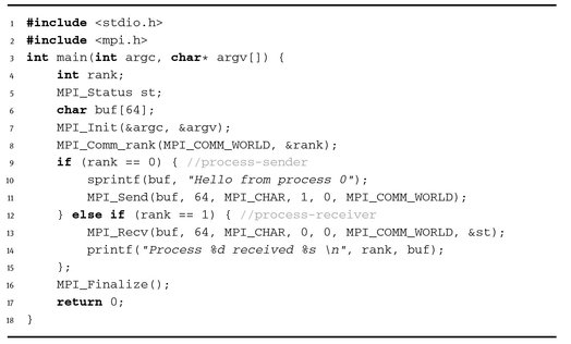
The output of the program is
Here the process with rank 0 puts the welcoming message in the buffer buf, which subsequently sends it to the process with rank 1. The process with rank 1 receives this message and prints it.
We apply functions of point exchanges to arrange data transfer in the above example. To send data the following function is used:

where buf is the starting address of the send buffer; count is the number of items in data; type is the datatype of sent items; dest is the rank of the destination process in the group associated with the communicator comm; tag is the data identifier; comm is the communicator.
In our example, we send the entire array buf. Since the array consists of 64 elements, count and type parameters are specified as 64 and the MPI_CHAR type, respectively. The dest argument determines the rank of the process for which the message is intended. The tag argument sets the so-called message tag, which is an integer that is passed along with the message and checked upon receiving. In the example, the rank of the receiver is 1, and the tag is 0.
To receive data, we employ the following function:

where buf is the starting address of the receive buffer; count is the number of received items; type is the datatype of received items; source is the rank of the process from which data was sent; tag is the data identifier; comm is the communicator; and status is attributes of the received message.
MPI provides additional data exchange functions which differ from each other in the ways they organize data exchange. Two of the functions described above implement the standard mode with blocking.
In functions with blocking, it is not possible to exit from functions until an exchange operation is completed. Therefore, sending functions are blocked until all sent data has been placed in a buffer (in some MPI implementations, it may be an intermediate system buffer or buffer of receiving process). On the other hand, receiving functions are blocked until all received data has been read from a buffer into the address space of the receiving process.
Both blocking and nonblocking operations support four execution modes. Table 4.1 presents the basic point-to-point communication functions.
Table 4.1. Point-to-point functions.
| Execution modes | Blocking | Nonblocking |
|---|---|---|
| Send | MPI-Send | MPI-Isend |
| Synchronous send | MPI-Ssend | MPI-Issend |
| Buffered send | MPI-Bsend | MPI-Ibsend |
| Ready send | MPI-Rsend | MPI-Irsend |
| Receive | MPI-Recv | MPI-Irecv |
In the table we can see how functions are named. To the name the basic functions Send/Recv, we add the following prefixes:
- – s (synchronous ) prefix indicates the synchronous data transfer mode. Here an operation will end only when receiving of data ends. The function is non-local.
- – B (buffered) prefix denotes the buffered data transfer mode. In this case a special function creates a buffer in the address space of the sending process which will be used in operations. The send operation terminates when data is placed in the buffer. The function is local.
- – R (ready) prefix indicates the ready data exchange mode. The send operation starts only when the receiving operation is initiated. The function is non-local.
- – I (immediate) prefix refers to nonblocking operations.
4.2.2 Data types
We must explicitly specify the type of data being sent for data exchange. MPI contains a large set of basic datatypes, which are essentially consistent with data types of the c and Fortran programming languages. Table 4.2 shows the basic MPI data types.
Table 4.2. Compliance between MPI and c datatypes.
| MPI type | C type |
|---|---|
| MPI_BYTE | |
| MPI_CHAR | signed char |
| MPI_DOUBLE | double |
| MPI_FLOAT | float |
| MPI_INT | int |
| MPI_LONG | long |
| MPI_LONG_DOUBLE | long double |
| MPI_PACKED | |
| MPI_SHORT | short |
| MPI_UNSIGNED_CHAR | unsigned char |
| MPI_UNSIGNED | unsigned int |
| MPI_UNSIGNED_LONG | unsigned long |
| MPI_UNSIGNED_SHORT | unsigned short |
However, if the system provides additional data types, MPI will also support them. For example, if the system supports complex variables with double precision DOUBLE COMPLEX, there will be the MPI_DOUBLE_COMPLEX data type. The MPI_BYTE and MPI_PACKED data types are used to transmit binary data without any conversion. In addition, it is possible to create new derived data types for a more precise and brief description of data.
4.3 Functions of collective interaction
Functions for collective interaction are discussed below. We consider examples of the matrix-vector multiplication and scalar product of vectors.
4.3.1 General information
A set of operations such as point-to-point communication is sufficient for any programming algorithm. However, MPI is not limited to this set of communication operations. One of the strong features of MPI is a wide set of collective operations which allow us to solve the most frequently arising problems in parallel programming. For example, we often need to send some variable or array from one process to all other processes. Of course, we can write a procedure for this using the Send/Recv functions. But it is more convenient to employ the collective MPI_Bcast operation, which implements the broadcast of data from one process to all other processes in the communication environment. This operation is very efficient, since the function is implemented employing internal capabilities of communication environment.
The main difference between collective and point-to-point operations is that collective operations always involve all processes associated with a certain communicator. Noncompliance with this rule leads to either crashing or hanging.
A set of collective operations includes the following:
- – the synchronization of all processes (MPI_Barrier);
- – collective communication operations including:
- – broadcasting of data from one process to all other processes in a communicator (MPI_Bcast);
- – gathering of data from all processes into a single array in the address space of the root process (MPI_Gather, MPI_Gatherv);
- – gathering of data from all processes into a single array and broadcasting of the array to all processes (MPI_Allgather, MPI_Allgatherv);
- – splitting of data into fragments and scattering them to all other processes in a communicator (MPI_Scatter, MPI_Scatterv);
- – combined operation of scatter/Gather (All-to-All), i.e. each process divides data from its transmit buffer and distributes fragments to all other processes while collecting fragments sent by other processes in its receive buffer (MPI_Alltoall, MPI_Alltoallv);
- – global computational operations (sum, min, max etc.) over the data located in different address spaces of processes;
- – saving a result in the address space of one process (MPI_Reduce);
- – sending a result to all processes (MPI_Allreduce);
- – the operation Reduce/Scatter (MPI_Reduce_scatter);
- – prefix reduction (MPI_Scan).
All communication routines, except for MPI_Bcast, are available in the following two versions:
- – the simple option, when all parts of transmitted data have the same length and occupy a contiguous area in the process’s address space;
- – the vector option, which provides more opportunities for the organization of collective communications in terms of both block lengths and data placement in the address spaces of processes. Vector variants have the v character at the end of the function name.
Distinctive features of collective operations are as follows:
- – a collective communication does not interact with point-to-point communications;
- – collective communications are performed with an implicit barrier synchronization. The function returns in each process only take place when all processes have finished the collective operation;
- – the amount of received data must be equal to the amount of sent data;
- – data types of sent and received data must be the same;
- – data have no tags.
Next we use some some examples to study collective operations in detail.
4.3.2 Synchronization function
The process synchronization function MPI_Barrier blocks the called process until all other processes of the group call this function. The function finishes at the same time in all processes (all processes overcome barrier simultaneously).
where comm is a communicator.
Barrier synchronization is employed for example to complete all processes of some stage of solving a problem, the results of which will be used in the next stage. Using barrier synchronization ensures that none of processes start the next stage before they are allowed to. The implicit synchronization of processes is performed by any collective function.
4.3.3 Broadcast function
The data broadcast from one process to all other processes in a communicator is performed using the MPI_Bcast function (see Figure 4.1). The process with the rank root sends a message from its buffer to all processes in the comm communicator.

where buffer is the starting address of the buffer; count is the number of items in data; datatype is the MPI datatype of sent data; root is the rank of the sending process; comm is the communicator.
After performing this function, each process in the comm communicator including the sender will receive a copy of sent data from the sender process root.
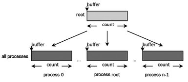
Fig. 4.1. Graphic interpretation of the MPI_Bcast function.
4.3.4 Data gathering functions
There are four functions for gathering data from all processes: MPI_Gather, MPI_Allgather, MPI_Gatherv, and MPI_Allgatherv. Each of these functions extends the possibilities of the previous one.
The MPI_Gather function assembles the data blocks sent by all processes into an array in the process with the root rank (Figure 4.2). The size of the blocks should be the same. Gathering takes place in the rank order, i.e. data sent by the i-th process from its buffer sendbuf is located in the i-th portion of the buffer recvbuf of the process root. The size of an array, where data is collected, should be sufficient to assemble them.
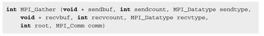
Here sendbuf is the starting address of sent data; sendcount is the number of items in data; sendtype is the datatype of sent data; recvbuf is the starting address of the receive buffer (used only in the receiving process root); recvcount is the number of elements received from each process (used only in the receiving process root); recvtype is the datatype of received elements; comm is the communicator.
The MPI_Allgather function described in Figure 4.3 is the same as MPI_Gather, but in this case all processes are receivers. Data sent by the i-th process from its buffer sendbuf is placed in the i-th portion of the buffer recvbuf of each process. After the operation, the contents of buffers recvbuf of all processes are the same.
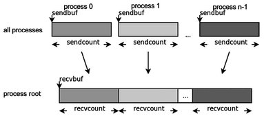
Fig. 4.2. Graphic interpretation of the MPI_Gather function.

sendbuf is the starting address of sent data; sendcount is the number of items in data; sendtype is the type of sent data; recvbuf is the starting address of the receive buffer; recvcount is the number of elements received from each process; recvtype is the datatype derived elements; comm is the communicator.

Fig. 4.3. Graphic interpretation of the MPI_Allgather function. In this sketch, the Y-axis is the group of processes and the X-axis indicates data blocks.
The MPI_Gatherv function (Figure 4.4) allows us to gather data blocks with different numbers of elements from each process, since the number of elements received from each process is defined individually using the array recvcounts. This feature also provides greater flexibility in locating data in receiving processes by introducing the new argument displs.

where sendbuf is the starting address of send buffer; sendcount is the number of items in data; sendtype is the datatype of sent data; recvbuf is the starting address of the receive buffer; recvcounts is an integer array (of the length equals the number of processes), where the value of i determines the number of elements that must be obtained from the i-th process; displs is an integer array (of the length equals the number of processes), where the value of i is the displacement of the i-th block of data with respect to recvbuf; recvtype is the datatype of received elements; root is the rank of the receiving process; comm is the communicator.
Messages are placed in the buffer of the receiving process in accordance with the sending process numbers. To be exact, data sent by the i-th process are placed in the address space of the root process, starting recvbuf + displs_i.

Fig. 4.4. Graphic interpretation of the MPI-Gatherv function.
The MPI_Allgatherv function is similar to the MPI_Gatherv function, except that gathering is performed by all processes. There is therefore no need for the root argument.

Where sendbuf is the starting address of the send buffer; sendcount is the number of items in data; sendtype is the data type of sent data; recvbuf is the starting address of the receive buffer; recvcounts is the integer array (of the length equals the number of processes), where the value of i determines the number of elements that must be obtained from the i-th process; displs is the integer array (of the length equals the number of processes), where the value of i is the displacement of the i-th block of data with respect to recvbuf; recvtype is the data type of received elements; comm is the communicator.
4.3.5 Data distribution functions
The functions for sending data blocks to all processes in a group are MPI_Scatter and MPI_Scatterv.
The MPI_Scatter function (see Figure 4.5) splits data from the send buffer of the root process into pieces with the size sendcount and sends the i-th part to the receive buffer of the process with the rank i (including itself). The root process uses two buffers (sending and receiving), so all function parameters are significant for the calling routine. On the other hand, the rest of the processes with the comm communicator are only recipients, and therefore their parameters which specify the send buffer are not significant.

Where sendbuf is the starting address of the send buffer (employed only by root); sendcount is the number of items sent to each process; sendtype is the data type of sent items; recvbuf is the starting address of the receive buffer; recvcount is the number of received items; recvtype is the datatype of received items; root is the rank of the sending process; comm is the communicator.
The data type of sent items sendtype must meet the type recvtype of received items. Also, the number of sent items sendcount must be equal to the number of received items recvcount. It should be noted that the value of sendcount at the root process is the number of elements sent to each process, not the total number. The scatter function is the inverse of the Gather function.

Fig. 4.5. Graphic interpretation of the MPI_Scatter function.
The MPI_Scatterv function (Figure 4.6) is a vector version of the MPI_Scatter function, which allows us to send a different number of elements to each process. The starting addresses of block elements sent to the i-th process are specified in the array of displacements displs, and the numbers of sent items are defined in the array sendcounts. This function is the inverse of the MPI_Gatherv function.

Where sendbuf is the starting address of the send buffer (used only by root); sendcounts is the integer array (of the length equals the number of processes) containing the number of elements sent to each process; displs is the integer array (of the length equals the number of processes), where the value of i determines the displacement of data sent by the i-th process with respect to sendbuf; sendtype is the data type of sent items; recvbuf is the starting address of the receive buffer; recvcount is the number of received items; recvtype is the data type of received items; root is the rank of the sending process; comm is the communicator.

Fig. 4.6. Graphic interpretation of the MPI_Scatterv function.
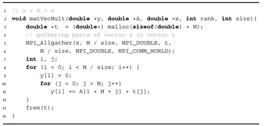
4.3.6 Matrix-vector multiplication
Now we discuss how to implement the parallel matrix-vector multiplication. We consider an N×N square matrix A and a vector b with N elements. The result of multiplying the matrix A by the vector b is a vector c with N elements.
We describe the parallel implementation of the algorithm, which splits the matrix into strips and calculates separate parts of the vector c within individual processes, and then brings the vector elements together.
Listing 4.4.


The partitioning of a matrix is performed using the scatter function. For convenience, the matrix is represented as a vector and its parts are scattered by separate processes. Since the vector b is employed by all processes, we apply the bcast function to send it. Finally, we gather the vector c in the process of rank 0.
4.3.7 Combined collective operations
The MPI_Alltoall function (see Figure 4.7) combines the Scatter and Gather functions and is an extension of the Allgather function, where each process sends different data to different recipients. The i-th process sends the j-th block of its sent buffer to the j-th process, which puts received data in the i-th block of its receive buffer. The amount of sent data must equal the amount of received data for each process.

Where sendbuf is the starting address of the send buffer; sendcount is the number of sent items; sendtype is data type of sent items; recvbuf is the starting address of the receive buffer; recvcount is the number of received items from each process; recvtype is the data type of received items; comm is the communicator.

Fig. 4.7. Graphic interpretation of the MPI-Alltoall function.
The MPI_Alltoallv function is a vector version of Alltoall. It sends and receives blocks of various lengths with more flexible placement of sent and received data.
4.3.8 Global computational operations
In parallel programming, mathematical operations on data blocks distributed among processors are called global reduction operations. In general, a reduction operation is an operation, one argument of which is a vector, and the result is a scalar value obtained by applying a mathematical operation to all components of the vector.
For example, if the address space of all processes of a group contains a variable var (there is no need to have the same value on each process), then we can apply the operation of global summation or the SUM reduction operation to this variable and obtain one value, which will contain the sum of all local values of this variable.
These operations are one of the basic tools for organizing distributed computations.
In MPI, the global reduction operations are available in the following versions:
- – MPI_Reduce – operation which saves a result in the address space of one process;
- – MPI_Allreduce – operation which saves a result in the address space of all processes;
- – MPI_Scan – prefix reduction operation which returns a vector as a result. The i-th component of this vector is the result of the reduction of the first i components of a distributed vector;
- MPI_Reduce_scatter – combined operation Reduce/scatter.
The MPI_Reduce function (Figure 4.8) works as follows. A global reduction operation specified by op is conducted on the first elements of the send buffer on each process, and the result is sent to the first element of the receive buffer of the root process. The same action is then done with the second element of the buffer, and so on.

Where sendbuf is the starting address of the send buffer; recvbuf is the starting address of the results buffer (used only in the root process); count is the number of elements in the send buffer; datatype is the data type of elements in the send buffer; op is the reduction operation; root is the rank of the receiving process; comm is the communicator.
As an op operation in the above description, it is possible to apply either predefined operations or user-defined operations. All predefined operations are associative and commutative. User-defined operations must be at least associative. The order of reduction is specified by the number of processes in a group. The types of elements must be compatible with the op operation. Table 4.3 presents predefined operations which can be used in the reduction function.

Fig. 4.8. Graphic interpretation of the MPI_Reduce function.
Table 4.3. Predefined reduction operations and compatible data types.
| Name | Operation | Datatype |
|---|---|---|
| MPI_MAX | Maximum | Integer |
| MPI_MIN | Minimum | Floating point |
| MPI_SUM | Sum | C integer |
| MPI_PROD | Product | Floating point, Complex |
| MPI_LAND | Logical AND | |
| MPI_LOR | Logical OR | C integer, Logical |
| MPI_LXOR | Logical exclusive OR | |
| MPI_BAND | Bit-wise AND | |
| MPI_BOR | Bit-wise OR | C integer |
| MPI_BXOR | Bit-wise exclusive OR | Byte |
| MPI_MAXLOC | Maximum and location of maximum | Special type for this function |
| MPI_MINLOC | Minimum and location of minimum | Special type for this function |
The MAXLOC and MINLOC functions are carried out with special pair types, each element of which stores two values: the value governing the search of the maximum or minimum, and the index of the element. MPI for c provides 6 such predefined types:
- – MPI_FLOAT_INT is float and int;
- – MPI_DOUBLE_INT is double and int;
- – MPl_LONG_INT is long and int;
- – MPI_2INT is int and int;
- – MPI_SHORT_INT is short and int;
- – MPI_LONG_DOUBLE_INT is long double and int.
The MPI_Allreduce function (Figure 4.9) stores the result of reduction in the address space of all processes, and so the root process is absent from the above list. The rest of the parameters are the same as in the previous function.

Where sendbuf is the starting address of the send buffer; recvbuf is the starting address of the receive buffer; count is the number of elements in the send buffer; datatype is the data type of elements in the send buffer; op is the reduce operation; comm is the communicator.

Fig. 4.9. Graphic interpretation of the MPI_Allreduce function.
TheMPl_Reduce_scatter function combines the reduction operation and the scattering of results.

Where sendbuf is the starting address of the send buffer; recvbuf is the starting address of the receive buffer; recvcounts is an array that specifies the size of sent data blocks; datatype is the data type of elements in the send buffer; op is the reduce operation; comm is the communicator.
The MPI_Reduce_scatter function (see Figure 4.10) differs from the MPI_Allreduce function so that the result of the operation is cut into disjoint parts according to the number of processes in a group, and the i-th part is sent to the i-th process. The lengths of these parts are defined by the third parameter, which is an array.
The MPI_Scan function (Figure 4.11) performs a prefix reduction. Function parameters are the same as in the MPI_Allreduce function, but results obtained by each process differ. The operation sends the reduction of the values of the send buffer of processes with ranks 0,1, ..., i to the receive buffer of the i-th process.

Fig. 4.10. Graphic interpretation of the MPI_Reduce_scatter function.

where sendbuf is the starting address of the send buffer; recvbuf is the starting address of the receive buffer; count is the number of elements in the send buffer; datatype is the data type of elements in the send buffer; op is the reduce operation; comm is the communicator.

Fig. 4.11. Graphic interpretation of the MPI_Scan function.
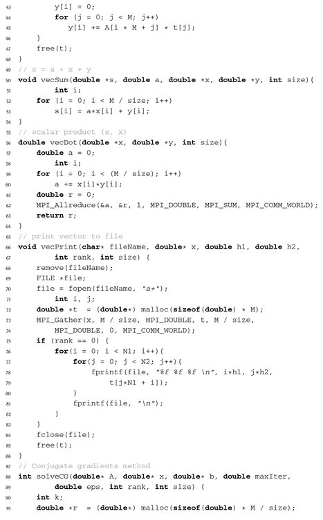
4.3.9 Scalar product of vectors
Let us consider the implementation of the scalar product of vectors. First, the sequential version of the scalar product is presented in Listing 4.5 below.
Listing 4.5.

In a parallel implementation of the scalar product, vectors are stored in a distributed manner, i.e. each process contains only part of a vector. Each process calculates the local scalar product of vectors. To derive the total scalar product, we need to use the reduction operation of summation (Figure 4.12).

Fig. 4.12. Sequential and parallel implementations of the scalar product of vectors.
Listing 4.6.

The above function can be employed to calculate the norm of vectors:
i.e. to take the square root of the scalar product.
4.4 Dirichlet problem for the Poisson equation
In the course of the book we consider the Dirichlet problem for the Poisson equation as the basic problem. The problem was described in detail in the sixth section of the previous chapter. Therefore, we provide only the problem formulation here. The approximation details and algorithm of iterative solution of the grid problem can be found in the chapter devoted to OpenMP technology. Here we construct a parallel implementation to solve the considered problem on the basis of MPI.
4.4.1 Problem formulation
In the unit square domain
we consider the Poisson equation
(4.1)
with Dirichlet boundary conditions
(4.2)
In our case, we put
(4.3)
4.4.2 Parallel algorithm
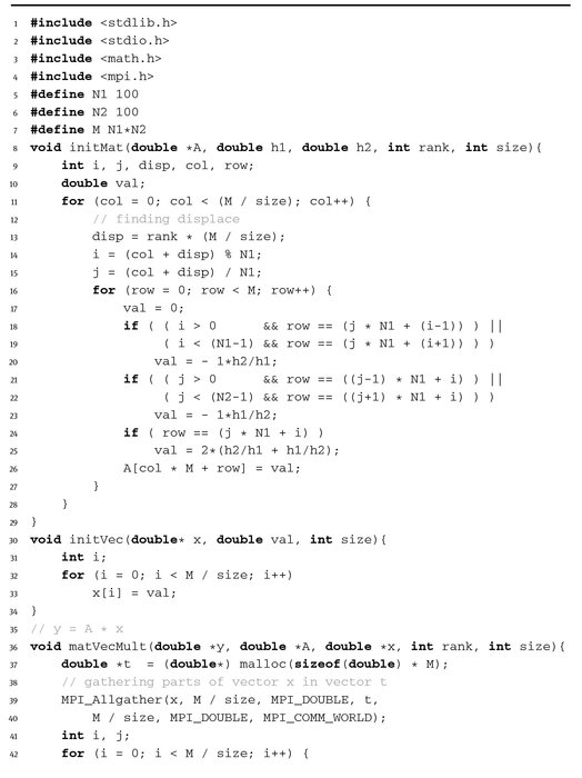
The parallel implementation of the above numerical algorithm requires essential modifications. First, we define the dimensions of problem as shown in Listing 4.7.
Listing 4.7.

The value M must be divisible by the number of running processes.
In the main function, we create matrix and vectors for the current process. Next, the five-diagonal matrix and the vector on the right are initialized. Further, we preset the initial guess and call the method of conjugate gradients for the numerical solution of the equations. After obtaining the solution we print the number of performed iterations and save the result to a file.
Listing 4.8.

The output file solution. txt can be visualized by gnuplot.
The implementation of the conjugate gradients method is conducted without using MPI functions.
Listing 4.9.


MPI functions appear in the scalar product of vectors as shown below in Listing 4.10.
Listing 4.10.

Next, the matrix-vector multiplication is shown in Listing 4.11.
Listing 4.11.
The matrix array A is filled-in in the initMat function.
Listing 4.12.

Here di sp is the displacement of a matrix block, which is defined as the multiplication of the process rank by the number of elements in the block.
The complete source code of the program is shown in Listing 4.13 below.
Listing 4.13.

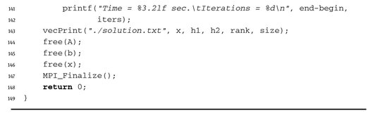
Here we use the required tolerance ε = 10-3 and the grid sizes N1 = 100, N2 = 100. 75 iterations are required to achieve the solution of the problem with the given accuracy (Figure 4.13).

Fig. 4.13. The solution of the Dirichlet problem (using gnuplot).
The output of the program for 1, 2, 4, 8 processes is as follows:
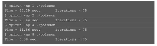
Note that the solution time decreases almost linearly when we increase the number of processes.