
Chapter 58. SSIS performance tips
Managing performance in SQL Server Integration Services (SSIS) can be an ever-changing battle that depends on many factors, both inside and outside the control of the SSIS developer. In this chapter, we will discuss a few techniques that will enable you to tune the Control Flow and the Data Flow elements of a package to increase performance.
Note
The following information is based on Integration Services in SQL Server 2005, Service Pack 2.
SSIS overview
SSIS packages are built around a control flow or a work surface to manage all activity within a package. The control flow is responsible for directing the execution path, as well as for managing predecessors, logging, and variables. The control flow also enables developers to use web services, interact with FTP sites, use custom scripts, and perform many more tasks that can all be linked together in serial or executed in parallel.
Data flow tasks are responsible for extracting, transforming, and loading data from a source to a destination. A source or a destination can be a database table, flat files, memory objects, custom objects, or other supported items. A generous list of components to transform data ships with SSIS and contains such items as row counters, aggregators, lookup transformations, and many more. Data flow tasks reside on the control flow and they can be the only task, or one of many.
Control flow performance
Tuning the control flow to perform as fast as possible depends on whether your tasks can run in parallel. If at all possible, set your control flow tasks to run parallel to each other to ensure that they start processing as soon as they can, and that they aren’t waiting for upstream tasks to finish.
You can control how many tasks can run in parallel using the MaxConcurrentExecutables property of the control flow. This property defaults to -1, which means that the number of parallel tasks processing at the same time will be limited to the number of logical processors plus 2. For example, if you have four processors on your server, SSIS will limit the number of parallel tasks to six. If your package in this example has eight parallel tasks, two of them will wait until one of the six executable slots opens up. You can change the MaxConcurrentExecutables property to a value greater than the number of processors on your server, but it still doesn’t mean that all tasks will process at the same time. Execution trees in a data flow task, for instance, can consume available executables, preventing other control flow tasks from executing.
Data flow performance
The data flow task is one of the core elements of SSIS. It is where data is extracted from one or more sources, possibly transformed, and then delivered to one or more destinations. As a result, this task has the most flexibility when it comes to tuning for performance. We will focus on five areas of the data flow that can be adjusted to maximize performance: source acquisition, transforming data, destination loading/updating, lookups, and the data flow in general.
Source acquisition performance
The data flow can work with data only as fast as it can acquire data from its source. If you can only select rows from a source database at a throughput of 10,000 rows per second, SSIS will be limited to processing no more than 10,000 rows per second as well. As shown in figure 1, the easiest way to determine how fast you can acquire data from a source is to hook the source component up to a Row Count transformation or a Copy Column transformation and execute the data flow task, taking note of the time it takes to extract your source data. I recommend repeating this process six or more times to establish an average baseline. To use the Row Count transformation, you’ll have to set up an SSIS variable to use in the transformation’s properties. The Copy Column transformation doesn’t have this requirement, and can be hooked up to the source component with no configuration needed.
Figure 1. An OLE DB Source component hooked up to a Row Count transformation

Once you have your extract average baseline, you’ll know the fastest possible speed at which SSIS can process your data. To ensure that you have the source properties tuned to achieve maximum performance, follow these tips:
- Make sure you are using current drivers for your connection. If there are multiple drivers available, be sure to test each one for the best performance, and ensure your packages use the optimum driver.
- Use SQL Command or SQL Command from Variable when setting the data access mode property of an OLE DB Source component and your source is a SQL Server database. This will execute the procedure sp_executesql. If you use a data access mode of Table or View or Table Name or View Name from Variable, SSIS will use the OPENROWSET() method to generate your results.
- Only select the columns you need in your data flow. This serves two purposes: it limits the amount of memory SSIS requires to store the data in its buffers, and it potentially buffers the source extract from source metadata changes. If you were to issue SELECT * FROM myTable instead, any column data type changes, additions, or removals can cause SSIS to fail validation and cause the package execution to fail.
- Add a WHERE clause to your source extract query to filter rows, returning only those rows that are required for processing. Of course, this only works if you are working with a source that’s queryable (such as SQL Server, Oracle, DB2, and Teradata) and not a flat file or other non-database source.
- Large sorts should be done in the source extract query if possible. This will cause the sort to run on the server and prevent SSIS from having to buffer all of the data to sort it, which on large datasets could result in swapping out to disk.
Data transformation performance
Transforming data is an extremely broad topic with a growing list of third-party components; I’ll only cover some of the general guidelines that should work across most transformation scenarios.
The first thing I recommend is building your transformations to perform all of the work you need to accomplish. Then, instead of adding a destination component, add a Row Count or a Copy Column transformation to assess the slowdown of your transformations, much like I demonstrated in the previous section. If your numbers are similar to your source acquisition baseline, you likely will not gain much by way of tuning your transformations. But if your numbers are much slower than your source acquisition baseline, you know you may have room for improvement.
To ensure your transformations have the best performance, some of the things to consider are
- Avoid unnecessary data type casting. If possible, cast to an appropriate data type in your source query.
- Some components such as Aggregate and Sort require that they receive all input rows before they can begin processing the rows. These are known as asynchronous components, and will block the flow of data to downstream components. You may want to consider implementing this logic in the source query if possible.
- If you are using a single Aggregate transformation with multiple outputs and those outputs are going to separate destinations, consider creating an aggregate for each destination. This will ensure that each aggregate will not have to wait on the lowest-granular aggregation to process, as is the case when using a single Aggregate transformation with multiple outputs.
Destination performance
The fastest destination component is the Raw File destination. This component stores its data in a format specific to SSIS and is extremely fast, with the only bottleneck being the speed of the disk you are writing to. This component is especially useful for exchanging data between data flows, as the metadata is stored in the raw file itself, which eliminates the need to specify the file layout when using the file as a source. This component can’t be configured to perform any faster than your disk allows.
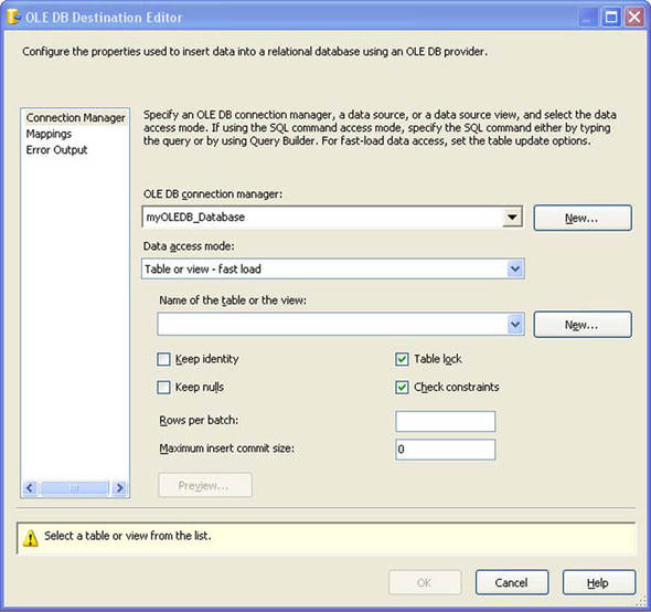
Perhaps the most common destination component in SSIS is the OLE DB Destination. This component allows the flexibility of issuing bulk inserts or row-by-row inserts. As shown in figure 2, to use the bulk insert function of this destination, select Table or view - fast load from the drop-down box of the data access mode property. The fast load option issues a bulk insert command at the destination and allows you to specify the number of rows to commit as a batch. The Maximum Insert Commit Size property defaults to 0, which tells SSIS to commit all incoming rows as a single batch. Setting this property to something other than 0 ensures that after SSIS has processed the set number of rows, it will issue a commit. If an insert error happens in a batch of rows, all of the rows in the batch are rolled back and the component raises an error. If you have the component set to redirect errors, the entire batch will be redirected, not just the row causing the error.
Figure 2. The OLE DB Destination fast load panel
Setting the commit size properly depends on what type of table you are inserting into and the number of rows being sent to the destination. If the number of rows is small, a commit size of 0 may work well for you. For a large number of rows, if the table doesn’t have a clustered index (for example, a heap table), the default commit size of 0 will generate the best performance. For a table that has a clustered index defined, all rows in the batch must be sorted up front to be inserted, which can cause performance issues depending on your memory specifications on the server. For that reason, on a table with a clustered index, it is best to set the commit size to a value appropriate for your environment (for example, 100,000 rows).
You may also find, on a table with a clustered index, that it is more beneficial to drop the index before inserting the rows and then rebuild the index after successfully completing all inserts. You’ll have to test this for each table to find the right solution.
The next component, OLE DB Command, is commonly used for updating destination tables. But, depending on your design, you may want to instead consider inserting your updates into a temporary table, and later, back on the control flow, issuing an Execute SQL task to perform a batch update. The OLE DB Command component executes each time a row passes through it, and for this reason it can become the slowest component in a data flow. Evaluate your options when considering using this component, and test them before making a decision that could negatively impact performance. This is unavoidable in some cases, such as when you are updating a table that you have a lookup selecting against in the same data flow, and you need the updated results to be reflected immediately.
The other commonly used destination is the flat file. Much like a raw file, its performance is dependent on the disk you are writing files to. This destination doesn’t store its metadata in the file, and as such, if you later want to read data from this file, you must define the column mappings in each package that uses the file as a source.
Perhaps the most effective destination component is the SQL Server destination. Use this component if your destination is SQL Server and the package resides on and is executed on the target SQL Server. This destination component bypasses the network layer when inserting into SQL Server, and is extremely fast as a result. The downside of using this destination is that it requires your data types to explicitly match the data types of the columns you are inserting into. Unlike the OLE DB destination, the SQL Server destination will not implicitly cast data types.
Lookup transformation performance
The Lookup transformation allows you to use a lookup table to achieve things such as checking to see whether a record exists and looking up a description of an item from a dimension table. It is a powerful transformation, and one that you’ll most likely use at some point.
The Lookup transformation has three primary settings: no cache, partial cache, and full cache. Each has benefits and drawbacks.
No Cache
This setting of the Lookup transformation forces a query against the lookup table (or query) for each row passing through it. As a result, this setting is very slow performing. The only performance gain you can get here is to make sure your lookup columns are indexed properly so as to avoid a table scan. Comparisons with this cache mode are done in the lookup table’s database, not SSIS. To use the no cache mode, select Enable Memory Restriction from the Advanced tab of the Lookup transformation.
Full Cache
In full cache mode, the Lookup transformation will attempt to store all lookup table rows in memory. SSIS will cache all rows before it starts processing data in the data flow. It is crucial that you select only the columns and rows that you need to perform your lookup, so that the memory storage is limited to the minimum amount possible. If you select more columns and rows than necessary, you risk causing SSIS to run out of memory, and because the Lookup transformation will not swap its memory out to disk, running out of memory is a fatal data flow error. The full cache mode is the fastest lookup mode; for this mode only, the equality rules are often different than those of a database engine. (For example, full cache mode uses case-sensitive rules even when the database may be set to case-insensitive.) To use the full cache mode, ensure that no options are selected on the Advanced tab of the Lookup transformation.
Partial Cache
The partial cache mode is a mix between no cache and full cache modes, in that it partially caches rows from the lookup table, with the size (in megabytes) of the cache limited to the cache size property of the Lookup transformation. Any rows that don’t match the cached dataset are sent to the database to see if they physically exist in the lookup table. Use this mode when using full cache would otherwise take up too much memory and you want to limit the upper memory requirements of the cache, or when you want to force the database to perform the equality checks and not SSIS. To use partial caching, ensure that Enable Memory Restriction is selected, and also ensure that either Enable Caching, Modify the SQL Statement, or both are selected.
General data flow performance
Each data flow has a few properties that should be evaluated for each implementation. DefaultBufferMaxRows and DefaultBufferSize are two properties that can drastically increase data flow performance if adjusted correctly.
DefaultBufferMaxRows specifies the maximum number of rows SSIS will place in a buffer. DefaultBufferSize specifies the default buffer size that SSIS uses in its calculations to determine how many rows to place in a buffer. The maximum allowable buffer size is 100 megabytes.
Tuning these two parameters will ensure that your data flow is optimized for its specific dataset. To determine the optimum setting, turn on the custom data flow logging event BufferSizeTuning. This event, when reading the resulting log file, will tell you how many rows were placed in the buffer. If your DefaultBufferMaxRows is set to the default of 10,000, and the BufferSizeTuning logging event is reporting only 2,000 rows were placed in the buffer, you’ll need to increase the DefaultBufferSize property to accommodate more rows or reduce the size of each row by eliminating unnecessary columns.
If your data flow has BLOB data in it, specifying a folder in the BLOBTempStoragePath property will allow you to change where BLOB data is spooled out to disk. Choosing a faster disk, instead of the disk specified in the TMP/TEMP environment variables, you may be able to increase data flow performance when working with BLOB data.
Note
SSIS always spools BLOB data to disk. Ensure that BLOBTempStoragePath is set to a disk that’s large enough to handle your BLOB data.
Summary
Tuning SSIS can be a time-consuming process and difficult to master. Each design situation will present unique challenges. To help you succeed in tuning your packages, be sure to
- Turn on package logging to help you understand what your packages are doing.
- Turn on the BufferSizeTuning custom event for your data flows in the logging provider to help you tune the DefaultBufferMaxRows and DefaultBufferSize properties.
- Always use SQL, if possible, to select from sources, and in your lookup transformations as well.
- Perform sort operations within the database if you can.
- Only select the columns you need in your data flow sources and lookup transformations.
About the author

Phil Brammer has more than nine years data warehousing experience in various technologies, including Red Brick, Teradata, and most recently, SQL Server. His specialty is in building extract, transform, and load (ETL) processes, using tools such as Informatica, and SQL Server Integration Services. He continues to play an active role in the Integration Services community via online resources as well as his technical blog site, http://ssistalk.com.