
Chapter 46. Using correlation to improve query performance
SQL Server doesn’t keep statistics on the correlation between nonclustered indexes and the clustered index (with the exception of correlation information between datetime columns, if the DATE_CORRELATION_OPTIMIZATION setting is turned on). Instead, the optimizer assumes it has a low correlation; it assumes that a range of nonclustered index values is scattered all over the clustered index.
This assumption affects the optimizer’s decision whether or not to use the nonclustered index. If there is a high correlation, the optimizer will overestimate the cost of using the nonclustered index, which can cause it to disqualify the index from the query plan evaluation, resulting in a suboptimal query plan. The performance difference can be big, even by orders of magnitude.
This chapter explains what it means to have a high correlation with the clustered index, why the optimizer can misjudge such situations, how to determine the correlation for your situation, and how to optimize your queries accordingly.
Note
In this chapter, I’ll assume that you’re familiar with indexes, and more specifically with the differences between clustered and nonclustered indexes. I’ll also assume that you have some experience with query tuning.
The purpose of the optimizer
It’s the optimizer’s job to find the best query plan for a query. What is best? For the optimizer, it’s the one that results in the shortest execution time.
In most cases, the performance of a typical query will be determined by the number of physical reads that are needed to satisfy the query. In a worst-case scenario, you have a cold cache, which means that no data or index pages are in cache. In a best-case scenario, you have a hot cache, and all relevant data is in memory.
If the page is cached, the data can be returned immediately. Otherwise, a physical read has to be issued to retrieve the page from disk. The duration of such a physical read depends on your storage subsystem. A physical read is typically several orders of magnitude slower than a read satisfied by the cache.
Physical reads come in two flavors: sequential reads and random reads. Although it depends on your storage subsystem and other factors like fragmentation, sequential reads are assumed to be significantly faster than random reads. Because of this, behind the scenes, the optimizer’s primary objective is to minimize the number of physical reads and writes, and to favor sequential reads over random reads.
This chapter has the same goal: to help you minimize the number of physical reads. If you want to optimize your queries for a hot cache, then this chapter won’t help you because the storage engine’s performance characteristics are different for cached data.
Correlation with the clustered index
The term correlation is used loosely here. We’re trying to determine the chance that two consecutive nonclustered index keys refer to the same data page. And we’re only considering tables that have a clustered index, although the same theory would also hold for heaps.
Low correlation
Most nonclustered indexes have a low correlation with the clustered index. Figure 1 shows such a situation for the Product table. It has a nonclustered index on Product Name and a clustered index on Product ID.
Figure 1. Low correlation index

The top row shows the nonclustered index values (the first 32 values). The letters in a block indicate the range of values. The number above a block indicates the number of values in that range. The bottom row shows the clustered index pages on which the row data is stored.
You can see that the first nine values in the nonclustered index refer to seven different pages in the clustered index, most of which are not shown. You can also see that if the storage engine would follow the nonclustered index, it would have to jump back and forth in the clustered index to retrieve the corresponding data.
If a range of nonclustered index values does not relate to a significantly smaller range of consecutive data pages, then for the intent and purpose of this chapter, it has a low correlation.
Figure 2 depicts a nonclustered index that has a high correlation with the clustered index. The clustered index is on WorkOrderID, the nonclustered index is on EndDate. WorkOrders with a later EndDate typically have a higher WorkOrderID, meaning they are correlated.
Figure 2. High correlation index
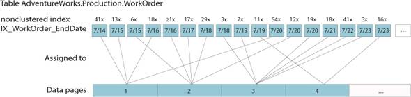
The figure shows that many of the days, each with tens of rows, are stored on just one or two pages. If a range of nonclustered index values relates to a significantly smaller number of consecutive data pages, then it has a high correlation.
When the optimizer does it right
Let’s look at an example. Listing 1 uses the AdventureWorks database on SQL Server 2005. It selects 88 rows (0.12 percent) of table WorkOrder. The table has 523 data pages, a clustered index on WorkOrderID, and it’s assumed that there’s a nonclustered index on EndDate.
Note
When you install the AdventureWorks database, there might not be an index on EndDate. I’ll assume you created it like this: CREATE INDEX IX_WorkOrder_EndDate ON Production.WorkOrder (EndDate).
Listing 1. Query to select WorkOrders for a 2-day date range
SELECT WorkOrderID, OrderQty, EndDate
FROM   Production.WorkOrder
WHERE  EndDate >= '20031101'
AND    EndDate <  '20031102'
The choice that the optimizer has to make is whether or not to use the nonclustered index. The optimizer has to choose one of the following options:
- Use the index on EndDate to locate the desired rows and then look up the corresponding rows through the clustered index.
- Scan the entire clustered index and filter out the unwanted rows.
Figure 3 shows the graphical query plan for listing 1. If you inspect the query plan, you will see that the optimizer estimates that 59 rows will be selected. If it uses the nonclustered index and clustered index seeks to look up the corresponding rows, it is estimated to cost a little over 59 reads, one read per row. If it had to scan the entire clustered index, it would cost a little over 523 reads, one read per page of the table. The optimizer makes the right choice, as displayed below.
Figure 3. Query plan that uses the nonclustered index

To determine the number of physical reads, you can use SET STATISTICS IO ON before running the query, or use SQL Profiler. If SQL Server’s cache is empty and you run this example, you will see only three physical reads and four read-ahead reads, a total of seven reads. (you could get slightly different results if you have worked with the AdventureWorks database before).
When the optimizer does it right again
Let’s change our example to select everything except this range of EndDates, as shown in listing 2. That would select 72,503 rows (99.88 percent).
Listing 2. Query to select all WorkOrders except for 2 days
SELECT WorkOrderID, OrderQty, EndDate
FROM   Production.WorkOrder
WHERE  EndDate <  '20031101'
OR     EndDate >= '20031102'
Because the number of selected rows exceeds the number of pages in the table—which was only 523—all potential query plans are estimated to require a little over 523 reads. In such a situation, the optimizer will always favor a clustered index scan, because that will use sequential reads, instead of random reads. Also, this avoids the risk of having to read the same page more than once.
Again the optimizer comes up with the optimal query plan, as displayed in figure 4.
Figure 4. Query plan that scans the entire clustered index

If SQL Server’s cache is empty and you run this example, you will see 1 physical read and 523 read-ahead reads, a total of 524 reads.
When the optimizer gets it wrong
Listing 3 shows a third example. This time, the range is limited to 2,844 rows (3.9 percent).
Listing 3. Query to select WorkOrders for a one-month date range
SELECT WorkOrderID, OrderQty, EndDate
FROM   Production.WorkOrder
WHERE  EndDate >= '20031101'
AND    EndDate <  '20031201'
The optimizer comes up with the same query plan as in listing 2, a clustered index scan (see figure 4). It assumes that all 523 data pages are needed to retrieve the data for these 2,844 rows. In other words, it assumes a low correlation between the nonclustered index and the clustered index.
If SQL Server’s cache is empty and you run this example, you will see the same 1 + 523 reads as in listing 2. The reality is that this range of 2,844 rows does not cover 523 pages, but only a fraction of that. Figure 2 visualizes this, you can use the accompanying T-SQL script to determine it, and the next chapter will prove it: the optimizer selected a suboptimal query plan, and the optimizer got it wrong! It should have chosen the query plan of figure 3, using the nonclustered index.
Correcting the optimizer
You can influence the optimizer’s behavior in several ways. The topics “Query Hint” and “Table Hint” in Books Online cover them.
The simplest method is to use the table hint INDEX. You use it in the FROM clause of the SELECT statement to specify the nonclustered index that should be used when accessing that table. The name of the nonclustered index on EndDate is called IX_WorkOrder_EndDate. Listing 4 shows the same query with the appropriate table hint.
Listing 4. Using an index hint
SELECT WorkOrderID, OrderQty, EndDate
FROM   Production.WorkOrder WITH (INDEX=IX_WorkOrder_EndDate)
WHERE  EndDate >= '20031101'
AND    EndDate <  '20031201'
If SQL Server’s cache is empty and you run this example, you will see 25 physical reads and 13 read-ahead reads, totaling 38 reads. The 13 read-ahead reads will be sequential reads, and the 25 physical reads might be random reads. Obviously, this is much faster than the 524 sequential reads of the optimizer’s original plan.
When to expect correlation
You might expect correlation in some common scenarios:
- Both the clustered index and the nonclustered index use ever-increasing key values; for example, an Orders table with a clustered index on an Identity OrderID, and a nonclustered index on the OrderDate. For a new order, both the OrderDate and the OrderID will have a higher value than the previous order. Other examples are the relation between an OrderDate and a DateDue, the relation between a name and its SoundEx value, and so on.
- When you use an Identity as a clustered index key, and you have imported a large percentage of the table data, and the import file was in sorted order; for example, if you have a Cities table with an Identity OrderID, and you import the city names in sorted order.
Determining correlation
You can use the accompanying T-SQL script to determine the correlation between index IX_WorkOrder_EndDate and the clustered index. You can modify the script to fit your needs, and test your own indexes for correlation.
Here is a short description of what the script does:
- Retrieves the distribution statistics of the clustered index (one row per value range).
- Determines the number of pages in the table, and uses that to estimate the number of pages per value range.
- Retrieves the distribution statistics of the nonclustered index (one row per value range).
- Determines the minimum and maximum clustered index key per nonclustered value range (a time-consuming step).
- Interpolates the number of consecutive clustered index pages per nonclustered value range, based on the minimum and maximum clustered index key within the range.
If the estimated number of pages for a range (the result of step 5) is lower than its number of rows, then there is a high correlation. For example, if there is a range with 100 values that is estimated to cover 25 consecutive pages, then reading those 100 rows through the nonclustered index could not result in 100 physical reads, but (if none of the pages are cached) would result in a maximum of (a little over) 25 physical reads.
If the number of pages for your query’s value range is lower than the total number of pages minus the number of nonclustered index pages, then it makes sense to correct the optimizer.
In other words, correct the optimizer if
consecutive pages covering your range < table pages - index pages
Summary
It’s quite common to have tables with a high correlation between a nonclustered index and the clustered index. In these situations, the optimizer tends to overestimate the cost of using the nonclustered index, which can lead to suboptimal query plans. The accompanying T-SQL script shows you how to determine if there is a strong correlation, and predicts whether adding an index hint could help your queries’ performance. As the examples have shown, such intervention can massively boost performance.
About the author

Gert-Jan Strik is an IT Architect in the Netherlands who has been working with SQL Server ever since Version 6.5, and in recent years has developed a particular interest in performance optimization and the inner workings of the optimizer and storage engine.