
Chapter 44. Does the order of columns in an index matter?
A single column index is straightforward. You may have heard it compared to the index in the back of a technical book. To find information in the book, say you want to learn more about how DBCC INPUTBUFFER is used, you look up DBCC INPUTBUFFER in the index. The index doesn’t contain the information on DBCC INPUTBUFFER; it has a pointer to the page where the command is described. You turn to that page and read about it. This is a good analogy for a single column, nonclustered index.
In Microsoft SQL Server, you can also create an index that contains more than one column. This is known as a composite index. A good analogy for a composite index is the telephone book.
Understanding the basics of composite indexes
A telephone book lists every individual in the local area who has a publicly available telephone number. It’s organized not by one column, but by two: last name and first name (ignoring the middle name that is sometimes listed but most often treated as an extension of the person’s first name).
To look up someone in the telephone book, you first navigate to the last name and then the first name. For example, to find Jake Smith, you first locate the Smiths. Then within the Smiths, you find Jake.
SQL Server can use composite indexes in a similar manner. Composite indexes contain more than 1 column and can reference up to 16 columns from a single table or view. The columns that compose a composite index can contain up to a combined 900 bytes.
Let’s consider some examples. Assume you have a Customers table as described in listing 1.
Listing 1. A sample Customers table
CREATE TABLE Customers
        (
         Customer_ID INT NOT NULL IDENTITY(1,1)
        ,Last_Name VARCHAR(20) NOT NULL
        ,First_Name VARCHAR(20) NOT NULL
        ,Email_Address VARCHAR(50) NULL
        );
The Customers table has a clustered index on Customer_ID and a nonclustered composite index on the Last_Name, First_Name. These are expressed in listing 2.
Listing 2. Creating indexes for the Customers table
CREATE CLUSTERED INDEX ix_Customer_ID
   ON Customers(Customer_ID);

CREATE INDEX ix_Customer_Name
   ON Customers(Last_Name, First_Name);
Finding a specific row
When we issue a query to SQL Server that retrieves data from the Customers table, the SQL Server query optimizer will consider the various retrieval methods at its disposal and select the one it deems most appropriate. Listing 3 provides a query in which we ask SQL Server to find a Customer named Jake Smith.
Listing 3. Finding a specific Customer row by Last_Name, First_Name
SELECT
   Last_Name
   ,First_Name
   ,Email_Address
FROM
   Customers
WHERE
   Last_Name = 'Smith' AND
   First_Name = 'Jake';
In the absence of an index, SQL Server would have to search through the entire table looking for the rows that satisfy this query. Because we have created a nonclustered index on the Last_Name and First_Name columns, SQL Server can use that index to quickly navigate to the selected rows. Figure 1 shows the query execution plan for the query.
Figure 1. Query execution plan for listing 1
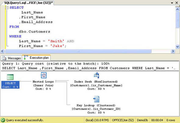
In the figure, we can see that SQL Server used an Index Seek operation on the nonclustered index named ix_Customer_Name to locate the rows selected by the query. To retrieve the additional non-indexed columns (Email_Address), a Key Lookup was used for each row. The results were put together in a nested Loop join and returned to the client.
You may have noticed that the WHERE clause in listing 1 provides the columns in the order that they appear in the ix_Customer_Name index. This is not a requirement in order for SQL Server to be able to use the index. If we reversed the order of the columns in the WHERE clause, SQL Server would still be able to use the index. But don’t take my word for it. Let’s look at another example to prove that this is indeed the case. Listing 4 shows the newly rewritten query that reverses the order of the columns in the WHERE clause.
Listing 4. Finding a specific Customer row by First_Name, Last_Name
SELECT
   *
FROM
   Customers
WHERE
   First_Name = 'Jake' AND
   Last_Name = 'Smith';
Issuing the query produces the query execution plan found in the figure 2 query execution plan for listing 4. The plan is identical to the prior example in which the WHERE clause listed the columns in order.
Figure 2. Query execution plan for listing 4

Finding a last name
In the prior example, we supplied values in the WHERE clause for both columns defined in the ix_Customer_Name index. The index is based on Last_Name, First_Name, and our query limited the results by providing a value for the Last_Name column and for the First_Name column.
Although this makes intuitive sense, a composite index’s usefulness is not limited to only those instances where this is true. SQL Server can use a composite index when only some of the index’s columns are provided. For example, consider the query depicted in listing 5.
Listing 5. Finding customers by Last_Name
SELECT
    Last_Name
   ,First_Name
   ,Email_Address
FROM
   Customers
WHERE
   Last_Name = 'Smith';
This query is similar to our prior example; however, notice that the WHERE clause now specifies only a Last_Name of Smith. We want to find all Smiths in our Customers table.
Looking at the query execution plan in figure 3 for the query specified in listing 5, we see that SQL Server did indeed use the ix_Customer_Name composite index. It performed an Index Seek operation to find the rows that satisfied the query. Then a Key Lookup operation was used to retrieve the non-indexed column information for each row that satisfied the query.
Figure 3. Query execution plan for listing 5

Returning to our telephone book analogy, we can see why this index was deemed efficient by the Query Optimizer. To find all of the Smiths in the telephone book, we’d navigate to the page that contains the first Smith and keep moving forward until we found the entry after Smith. SQL Server resolved the query in a similar manner using the ix_Customer_Name index.
Finding a first name
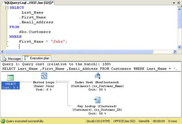
The prior demonstration proved that SQL Server can use a composite index even though only some of the columns of the index are specified in the WHERE clause. But does it matter which columns are specified? To find out, let’s consider another example.
In this example, we’ll change what we are specifying in our search criteria. We’ll no longer look for all Customers with a last name of Smith. Instead, we’ll search for all Customers with a first name of Jake. Listing 6 shows our new query.
Listing 6. Finding Customers with a first name of Jake
SELECT
    Last_Name
   ,First_Name
   ,Email_Address
FROM
   Customers
WHERE
   First_Name = 'Jake';
When we run this query in SQL Server Management Studio and examine the query execution plan shown in figure 4, we can see that SQL Server no longer is able to use an Index Seek operation to specifically locate the rows that satisfy the query. Instead it must resort to an Index Scan operation.
Figure 4. Query execution plan for listing 6
Why is that? Let’s consider our telephone book analogy again. How useful would the telephone book be if you need to find everyone with a first name of Jake? Not very. You’d have to start on the first page of the book and look through every entry to see if the person’s first name is Jake. Why? Because the telephone book is not organized by first name; it’s organized by last name, first name.
The same holds true for SQL Server. An index cannot be used to seek rows of data when the first column of the index is not specified in the WHERE clause.
That’s not to say that the index is completely worthless for queries such as the one defined in listing 6. One the contrary, it can still improve performance significantly. Looking again at figure 4, we see that a nonclustered index scan on ix_Customer_Name was used to resolve the query. In an index scan SQL Server examines every entry in the index to see if it matches the specified criteria. This may sound like an expensive operation, but it’s much better than the alternative, a clustered index scan, also known as a table scan.
To see that this is the case, let’s look again at the properties of the nonclustered index scan from our last example. Let’s run the query again. This time we’ll turn on STATISTICS IO so that we can measure the logical and physical reads required to satisfy the query. Listing 7 shows how to turn the setting on.
Listing 7. Turning STATISTICS IO on
SET STATISTICS IO ON
Before issuing our query, let’s make sure we are starting with a clean state by clearing the procedure cache and freeing up memory. This is shown in listing 8.
Listing 8. Using DBCC to drop the procedure cache and free memory
DBCC DROPCLEANBUFFERS
DBCC FREEPROCCACHE
Now, let’s rerun the query and look at the logical and physical reads required to retrieve the results. This is shown in figure 5.
Figure 5. Reads required for listing 6
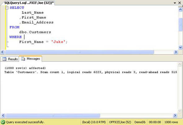
Notice that the query required one pass through the index. That’s the Scan Count of 1. It’s also required 6,223 logical reads and 3 physical reads to retrieve the information from the ix_Customer_Name index pages. A logical read occurs when SQL Server requests a page from the buffer cache. A physical read occurs when SQL Server must go to disk to retrieve the page.
Let’s compare these figures to that which would occur if the ix_Customer_Name nonclustered index were not there. To do this, we’ll drop the index, as shown in listing 9.
Listing 9. Dropping the ix_Customer_Name index
DROP INDEX ix_Customer_Name ON dbo.Customers
With the index gone, let’s re-issue the query in listing 6. The results are shown in figure 6.
Figure 6. Reads required for listing 6 without the ix_Customer_Name index

Without the benefit of the ix_Customer_Name index, SQL Server still required only one pass through the table to resolve the query. But the logical reads exploded to 14,982 and the physical reads ballooned to 109! Why? Let’s look at the query execution plan to see; it’s shown in figure 7.
Figure 7. Query execution plan for listing 6 without the ix_Customer_Name index

The figure shows that a clustered index scan, or a table scan, was required to resolve the query. That means that each row of the table had to be read.
Compared to the table, a nonclustered index typically is contained on far fewer data pages and therefore requires far fewer reads. And as we know, disk I/O is a major contributing factor to poor performance. So a nonclustered index scan is still far more efficient than scanning the entire table.
Summary
Indexes that include multiple columns, known as composite indexes, allow SQL Server to efficiently search for rows in a table or view. Understanding how the query optimizer can use these indexes allows you to create queries that can improve performance and reduce resource contention.
About the author

Joe Webb, a Microsoft SQL Server MVP, serves as Chief Operating Manager for WebbTech Solutions, a Nashville-based IT consulting company. He has over 15 years of industry experience and has consulted extensively with companies in the areas of business process analysis and improvements, database design and architecture, software development, and technical training.
In addition to helping his consulting clients, Joe enjoys writing and speaking at technical conferences. He has delivered over 50 sessions at conferences in Europe and North America and has authored two other books.
Joe served for six years on the Board of Directors for the Professional Association for SQL Server (PASS), an international user group with 30,000 members worldwide. He culminated his tenure on the board by serving as the Executive Vice President of Finance for the organization. Joe also volunteers his time by serving on the MBA Advisory Board for Auburn University and the Computer Science Advisory Committee for Nashville State Community College.
When he’s not consulting, Joe enjoys spending time with his family and tending to the animals and garden on his small farm in middle Tennessee. He may be reached at [email protected].