9

Performance Optimization for Real-Time Inference

Machine Learning (ML) and Deep Learning (DL) models are used in almost every industry, such as e-commerce, manufacturing, life sciences, and finance. Due to this, there have been meaningful innovations to improve the performance of these models. Since the introduction of transformer-based models in 2018, which were initially developed for Natural Language Processing (NLP) applications, the size of the models and the datasets required to train the models has grown exponentially. Transformer-based models are now used for forecasting as well as computer vision applications, in addition to NLP.

Let’s travel back in time a little to understand the growth in size of these models. Embeddings from Language Models (ELMo), which was introduced in 2018, had 93.6 million parameters, while the Generative Pretrained Transformer model (also known as GPT-3), in 2020, had 175 billion parameters. Today, we have DL models such as Switch Transformers (https://arxiv.org/pdf/2101.03961.pdf) with more than 1 trillion parameters. However, the speed of innovation of hardware to train and deploy such models is not catching up with the speed of innovation of large models. Therefore, we need sophisticated techniques to train and deploy these models in a cost-effective yet performant way.

One way to address this is to think in terms of reducing the memory footprint of the model. Moreover, many inference workloads must provide flexibility, high availability, and the ability to scale as enterprises serve millions or billions of users, especially for real-time or near real-time use cases. We need to understand which instance type and how many instances to use for deployment. We should also understand the key metrics based on which we will optimize the models.

Therefore, to collectively address the preceding scenarios, in this chapter, we will dive deep into the following topics:

• Reducing the memory footprint of DL models
• Key metrics for optimizing models
• Choosing instance type, load testing, and performance tuning for models
• Observing results

Important note

For details on training large DL models, please refer to Chapter 6, Distributed Training of Machine Learning Models, where we cover the topic in detail along with an example.

Technical requirements

You should have the following prerequisites before getting started with this chapter:

• A web browser (for the best experience, it is recommended that you use the Chrome or Firefox browser)
• Access to the AWS account that you used in Chapter 5, Data Analysis
• Access to the SageMaker Studio development environment that we created in Chapter 5, Data Analysis
• Example Jupyter notebooks for this chapter are provided in the companion GitHub repository (https://github.com/PacktPublishing/Applied-Machine-Learning-and-High-Performance-Computing-on-AWS/tree/main/Chapter09)

Reducing the memory footprint of DL models

Once we have trained the model, we need to deploy the model to get predictions, which are then used to provide business insights. Sometimes, our model can be bigger than the size of the single GPU memory available on the market today. In that case, you have two options – either to reduce the memory footprint of the model or use distributed deployment techniques. Therefore, in this section, we will discuss the following techniques to reduce the memory footprint of the model:

• Pruning
• Quantization
• Model compilation

Let’s dive deeper into each of these techniques, starting with pruning.

Pruning

Pruning is the technique of eliminating weights and parameters within a DL model that have little or no impact on the performance of the model but a significant impact on the inference speed and size of the model. The idea behind pruning methods is to make the model’s memory and power efficient, reducing the storage requirement and latency of the model. A DL model is basically a neural network with many hidden layers connected to each other. As the size of the model increases, the number of hidden layers, parameters, and weight connections between the layers also increases. Therefore, pruning methods tend to remove unused parameters and weight connections without too much bearing on the accuracy of the model, as shown in Figure 9.1 and Figure 9.2. Figure 9.1 shows a neural network before pruning:

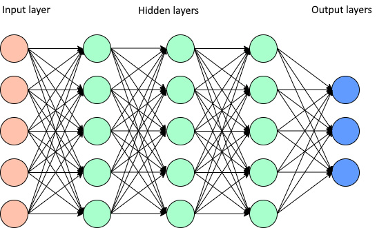
Figure 9.1 – Simple neural network before pruning

Figure 9.2 shows the same neural network after pruning:

Figure 9.2 – Simple neural network after pruning

Now that we’ve covered pruning, let’s take a look at quantization next.

Quantization

To train a neural network, data is first passed through the network in a forward pass, which calculates the activations, and then a backward pass, which uses the activations to calculate the gradients. The activations and gradients are usually stored in floating point 32, which takes 4 bytes of memory. When you have models with billions or trillions of parameters, this number is pretty significant. Therefore, quantization is a technique that reduces the model size by decreasing the precision of weights, biases, and activations of the model, such as floating point 16 or 8, or even to integer 8, which takes significantly less memory. For example, the GPT-J-6B model, which has 6 billion trainable parameters, takes about 23 GB of memory, as shown in Figure 9.3.

Figure 9.3 shows the number of parameters and size of the model when loaded from the Hugging Face library:

Figure 9.3 – The model size and number of parameters for the GPT-J-6B model

The same model when loaded with 16-bit floating point precision takes about 11 GB of memory, which is a memory reduction of about half, and can fit into a single GPU memory for inference as shown in Figure 9.4:

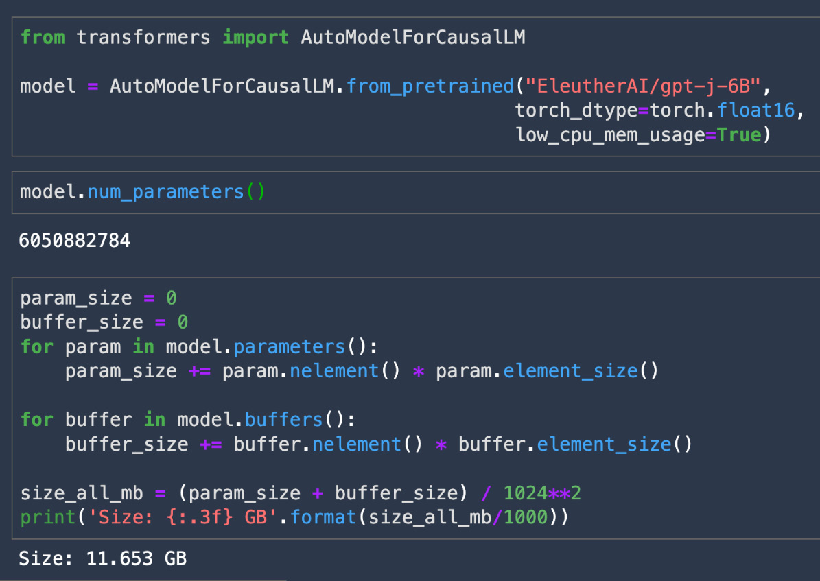
Figure 9.4 – The model size and number of parameters for the GPT-J-6B model with FP16 precision

As shown in Figure 9.3 and Figure 9.4, quantization can be a useful technique for reducing the memory footprint of the model.

Now, let’s take a look at another technique, called model compilation.

Model compilation

Before we go into model compilation, let’s first understand compilation.

Compilation is the process of converting a human-readable program that is a set of instructions into a machine-readable program. This core idea is used as a backbone for many programming languages, such as C, C++, and Java. This process also introduces efficiencies in the runtime environment of the program, such as making it platform-independent, reducing the memory size of the program, and so on. Most programming languages come with a compiler, which is used to compile the code into a machine-readable form as writing a compiler is a tedious process and requires a deep understanding of the programming language as well as the hardware.

A similar idea is used for compiling ML models. With ML, compilers place the core operations of the neural network on GPUs in a way that minimizes overhead. This reduces the memory footprint of the model, improves the performance efficiency, and makes it hardware agnostic. The concept is depicted in Figure 9.5, where the compiler takes a model developed in PyTorch, TensorFlow, XGBoost, and so on, converts it into an intermediate representation that is language agnostic, and then converts it into machine-readable code:

Figure 9.5 – High-level model compilation process

Model compilation eliminates the effort required to fine-tune the model for the specific hardware and software configurations of each platform. There are many frameworks available today using which you can compile your models, such as TVM and ONNX, each with its own pros and cons.

Note

Discussing compilers in detail is out of the scope of this book. For details on TVM, refer to this link: https://tvm.apache.org/. And for details about ONNX, refer to this link: https://onnx.ai/.

Let’s discuss a feature of Amazon SageMaker called SageMaker Neo, which is used to optimize ML models for inference on multiple platforms. Neo automatically optimizes models written in various frameworks, such as Gluon, Keras, PyTorch, TensorFlow, and so on, for inference on different platforms, such as Linux and Windows, as well as many different processors. For a complete list of frameworks or processors supported by Neo, please refer to this link: https://docs.aws.amazon.com/sagemaker/latest/dg/neo-supported-devices-edge.html.

The way Neo works is that it will first read the model, convert the framework-specific operations and functions into an intermediate representation that is framework agnostic, and finally, apply a series of optimizations. It will then generate binary code for optimized operations, write it to the shared object library and save the model definition and parameters in separate files (https://docs.aws.amazon.com/sagemaker/latest/dg/neo.html).

It also provides a runtime for each target platform that loads and executes the compiled model. Moreover, it can optimize the models with parameters either in floating point 32 (FP32), quantized into integer 8 (INT8), or in floating point 16 (FP16). It can improve the model’s performance up to 25 times with less than one-tenth of the footprint of a DL framework such as TensorFlow or PyTorch. To understand this further, let’s take a pretrained image classification model from PyTorch and optimize it using SageMaker Neo.

Note

We touched on SageMaker Neo in Chapter 8, Optimizing and Managing Machine Learning Models for Edge Deployment. Here, we will be using the same example to explain it in detail. For the full code, refer to the GitHub link: https://github.com/PacktPublishing/Applied-Machine-Learning-and-High-Performance-Computing-on-AWS/blob/main/Chapter08/sagemaker_notebook/1_compile_resnet_model_egde_manager.ipynb.

Follow these steps to optimize a pretrained model using SageMaker Neo:

1. First, we will download a pretrained model from the PyTorch library as shown in the following code snippet:

   …

   from torchvision.models import resnet18, ResNet18_Weights

   #initialize the model

   weights = ResNet18_Weights.DEFAULT

   model = resnet18(weights)

   …
2. Next, we need to save the model in model.tar.gz format, which SageMaker requires, specify the input data shape, and upload the model to Amazon S3:

   …

   torch.save(model.state_dict(),

              './output/resnet18-model.pt')

   with tarfile.open("model.tar.gz", "w:gz") as f:

       f.add("model.pth")

   input_tensor = torch.zeros([1, 3, 224, 224])

   model_uri = sagemaker_session.upload_data(

       path="model.tar.gz", key_prefix=key_prefix)

   print("S3 Path for Model: ", model_uri)

   …
3. Once we have the model in SageMaker format, we will prepare the parameters required for model compilation. Most importantly, you need to mention the target_device parameter, as based on it, SageMaker Neo will compile the model for the particular hardware on which the model will be deployed:

   …

   compilation_job_name = name_from_base("image-classification-neo")

   prefix = key_prefix+'/'+compilation_job_name+"/model"

   data_shape = '{"input0":[1,3,224,224]}'

   target_device = "ml_c5"

   framework = "PYTORCH"

   framework_version = "1.8"

   compiled_model_path = "s3://{}/{}/output".format(bucket, compilation_job_name)

   print("S3 path for compiled model: ", compiled_model_path)

   …
4. Next, we will declare the PyTorchModel object provided by SageMaker, which will have the necessary configurations, such as the model’s S3 path, the framework version, the inference script, the Python version, and so on:

   …

   from sagemaker.pytorch.model import PyTorchModel

   from sagemaker.predictor import Predictor

   sagemaker_model = PyTorchModel(

       model_data=model_uri,

       predictor_cls=Predictor,

       framework_version=framework_version,

       role=role,

       sagemaker_session=sagemaker_session,

       entry_point="inference.py",

       source_dir="code",

       py_version="py3",

       env={"MMS_DEFAULT_RESPONSE_TIMEOUT": "500"},

   )

   …
5. Finally, we will use the PyTorchModel object to create the compilation job and deploy the compiled model to the ml.c5.2xlarge instance, since the model was compiled for ml.c5 as the target device:

   …

   sagemaker_client = boto3.client("sagemaker",

       region_name=region)

   target_arch = "X86_64"

   target_os = 'LINUX'

   response = sagemaker_client.create_compilation_job(

       CompilationJobName=compilation_job_name,

       RoleArn=role,

       InputConfig={

           "S3Uri": sagemaker_model.model_data,

           "DataInputConfig": data_shape,

           "Framework": framework,

       },

       OutputConfig={

           "S3OutputLocation": compiled_model_path,

           "TargetDevice": 'jetson_nano',

           "TargetPlatform": {

               "Arch": target_arch,

               "Os": target_os

           },

       },

       StoppingCondition={"MaxRuntimeInSeconds": 900},

   )

   print(response)

   …
6. Once the model has finished compiling, you can then deploy the compiled model to make inference. In this case, we are deploying the model for real-time inference as an endpoint:

   …

   predictor = compiled_model.deploy(

       initial_instance_count=1,

       instance_type="ml.c5.2xlarge")

   …

Note

For more details on different deployment options provided by SageMaker, refer to Chapter 7, Deploying Machine Learning Models at Scale.

7. Now, once the model is deployed, we can invoke the endpoint for inference as shown in the following code snippet:

   …

   import numpy as np

   import json

   with open("horse_cart.jpg", "rb") as f:

       payload = f.read()

       payload = bytearray(payload)

   response = runtime.invoke_endpoint(

       EndpointName=ENDPOINT_NAME,

       ContentType='application/octet-stream',

       Body=payload,

       Accept = 'application/json')

   result = response['Body'].read()

   result = json.loads(result)

   print(result)

   …

Note

Since we have deployed the model as a real-time endpoint, you will be charged for the instance on which the model is deployed. Therefore, if you are not using the endpoint, make sure to delete it using the following code snippet.

8. Use the following code snippet to delete the endpoint, if you are not using it:

   …

   # delete endpoint after testing the inference

   import boto3

   # Create a low-level SageMaker service client.

   sagemaker_client = boto3.client('sagemaker',

                                   region_name=region)

   # Delete endpoint

   sagemaker_client.delete_endpoint(

       EndpointName=ENDPOINT_NAME)

   …

Now that we understand how to optimize a model using SageMaker Neo for inference, let’s talk about some of the key metrics that you should consider when trying to improve the latency of models. The ideas covered in the next section apply to DL models, even when you are not using SageMaker Neo, as you might not be able to compile all models with Neo. You can see the supported models and frameworks for SageMaker Neo here: https://docs.aws.amazon.com/sagemaker/latest/dg/neo-supported-cloud.html.

Key metrics for optimizing models

When it comes to real-time inference, optimizing a model for performance usually includes metrics such as latency, throughput, and model size. To optimize the model size, the process typically involves having a trained model, checking the size of the model, and if it does not fit into single CPU/GPU memory, you can choose any of the techniques discussed in the Reducing the memory footprint of DL models section to prepare it for deployment.

For deployment, one of the best practices is to standardize the environment. This will involve the use of containers to deploy the model, irrespective of whether you are deploying it on your own server or using Amazon SageMaker. The process is illustrated in Figure 9.6.

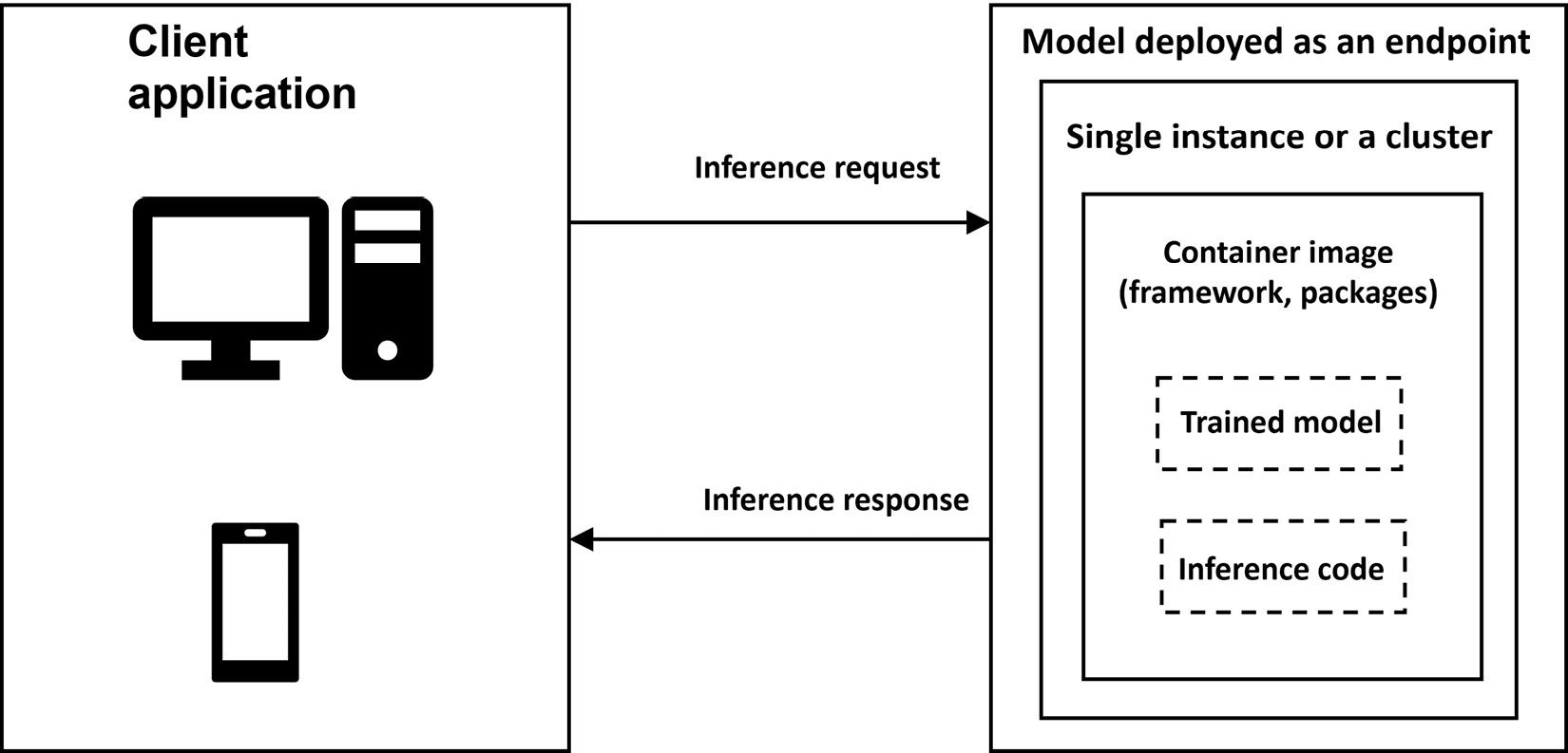
Figure 9.6 – Model deployed as a real-time endpoint

To summarize, we will first prepare the model for deployment, select or create a container to standardize the environment, followed by deploying the container on an instance(s). Therefore, to optimize the model’s performance, it is important to look for both inference and instance metrics. Inference metrics include the following:

• Invocations: The number of requests sent to the model endpoint. You can get the total number of requests by using the sum statistics in Amazon CloudWatch, which monitors the AWS resources or applications that you run on AWS in real time, including SageMaker (https://docs.aws.amazon.com/AmazonCloudWatch/latest/monitoring/WhatIsCloudWatch.html).
• Invocations per instance: If your model is deployed on more than one machine, then it’s important to understand the number of invocations sent to a model on each instance.
• Model latency: This is the time interval taken by a model to respond. It includes the local communication time taken to send the request, for the model to complete the inference in the container, and to get the response from the container of the model:

model latency = request time + inference time taken by the model + response time from the container

• Overhead latency: This is the time taken to respond after the endpoint has received the request minus the model latency. It can depend on multiple factors, such as request size, request frequency, authentication/authorization of the request, and response payload size.
• Maximum Invocations: This is the maximum number of requests to an endpoint per minute.
• Cost per hour: This gives the estimated cost per hour for your endpoint.
• Cost per inference: This provides the estimated cost per inference on your endpoint.

Note

Cost metrics provide the cost in US dollars.

In addition to inference metrics, you should also consider optimizing for instance metrics such as GPU utilization, GPU memory, CPU utilization, and CPU memory based on the instance type selected. Amazon SageMaker offers more than 70 instances from which you can choose to deploy your model. This brings up an additional question on how to determine which instance type and the number of instances to select for deploying the model in order to achieve your performance requirements. Let’s discuss the approach for selecting the optimal instance for your model in the next section.

Choosing the instance type, load testing, and performance tuning for models

Traditionally, based on the model type (ML model or DL model) and model size, you can make a heuristic guess to test the model’s performance on a few instances. This approach is fast but might not be the best approach. Therefore, in order to optimize this process, alternatively, you can use the Inference Recommender feature of Amazon SageMaker (https://docs.aws.amazon.com/sagemaker/latest/dg/inference-recommender.html), which automates the load testing and model tuning process across the SageMaker ML instances. It helps you to deploy the ML models on the optimized hardware, based on your performance requirements, at the lowest possible cost.

Let’s take an example by using a pretrained image classification model to understand how Inference Recommender works. The following steps outline the process of using Inference Recommender:

1. Determine the ML model details, such as framework and domain. The following is a code snippet for this:

   …

   # ML model details

   ml_domain = "COMPUTER_VISION"

   ml_task = "IMAGE_CLASSIFICATION"

   …
2. Take a pretrained model and package it in the compressed TAR file (*.tar.gz) format, which SageMaker understands, and upload the model to Amazon S3. If you have trained the model on SageMaker, then you can skip this step:

   …

   from torchvision.models import resnet18, ResNet18_Weights

   #initialize the model

   weights = ResNet18_Weights.DEFAULT

   model = resnet18(weights)

   torch.save(model.state_dict(), './output/resnet18-model.pt')

   with tarfile.open("model.tar.gz", "w:gz") as f:

       f.add("model.pth")

   input_tensor = torch.zeros([1, 3, 224, 224])

   model_uri = sagemaker_session.upload_data(path="model.tar.gz", key_prefix=key_prefix)

   print("S3 Path for Model: ", model_uri)

   …
3. Select the inference container, which can be a prebuilt Docker container provided by AWS or your own custom container. In our example, we are fetching a prebuilt PyTorch container image provided by AWS:

   …

   instance_type = "ml.c5.xlarge"  # Note: you can use any CPU-based instance type here, this is just to get a CPU tagged image

   container_uri = image_uris.retrieve(

       "pytorch",

       region,

       version=framework_version,

       py_version="py3",

       instance_type=instance_type,

       image_scope="inference",

   )

   container_uri

   …
4. Create a sample payload. In our example, we have images in .jpg format, compress them in a TAR file, and upload it to Amazon S3. In this example, we are only using four images, but it’s recommended to add a variety of samples, which is reflective of your actual payloads:

   !wget https://multimedia-commons.s3-us-west-2.amazonaws.com/data/images/139/019/1390196df443f2cf614f2255ae75fcf8.jpg -P /sample-payload

   !wget https://multimedia-commons.s3-us-west-2.amazonaws.com/data/images/139/015/1390157d4caaf290962de5c5fb4c42.jpg -P /sample-payload

   !wget https://multimedia-commons.s3-us-west-2.amazonaws.com/data/images/139/020/1390207be327f4c4df1259c7266473.jpg  -P /sample-payload

   !wget https://multimedia-commons.s3-us-west-2.amazonaws.com/data/images/139/028/139028d865bafa3de66568eeb499f4a6.jpg  -P /sample-payload

Compress the payload in TAR format as shown in the following code snippet and upload it to S3:

cd ./sample-payload/ && tar czvf ../{payload_archive_name} *

Once, we have the payload in TAR format, let’s use the following code snippet to upload it to Amazon S3:

…
sample_payload_url = sagemaker_session.upload_data(path=payload_archive_name, key_prefix="tf_payload")
…

5. Register the model in the model registry, which is used to catalog models for production, manage model versions, associate metadata, manage the approval status of the model, deploy models to production, and automate the model deployment process (https://docs.aws.amazon.com/sagemaker/latest/dg/model-registry.html). Registering a model in the model registry is a two-step process, as shown here:
   1. Create a model package group, which will have all the versions of the model:

      …

      model_package_group_input_dict = {

      "ModelPackageGroupName": model_package_group_name,

      "ModelPackageGroupDescription": model_package_group_description,

      }

      create_model_package_group_response = sm_client.create_model_package_group(**model_package_group_input_dict)

      …
   2. Register a model version to the model package group. To get the recommended instance type, you have two options – either you can specify a list of instances that you want Inference Recommender to use or you can not provide the instance list and it will pick the right instance based on the ML domain and ML task. For our example, we will use a list of common instance types used for image classification algorithms. This involves three steps.
   3. First, create an input dictionary with configuration for registering the model, as shown in the following code snippet:

      …

      model_approval_status = "PendingManualApproval"

      # provide an input dictionary with configuration for registering the model

      model_package_input_dict = {

          "ModelPackageGroupName": model_package_group_name,

          "Domain": ml_domain.upper(),

          "Task": ml_task.upper(),

          "SamplePayloadUrl": sample_payload_url,

          "ModelPackageDescription": model_package_description,

          "ModelApprovalStatus": model_approval_status,

      }# optional – provide a list of instances

      supported_realtime_inference_types = ["ml.c5.xlarge", "ml.m5.large", "ml.inf1.xlarge"]

      ...
   4. The second step is to create a model inference specification object, which will consist of providing details about the container, framework, model input, content type, and the S3 path of the trained model:

      #create model inference specification object

      modelpackage_inference_specification = {

          "InferenceSpecification": {

              "Containers": [

                  {

                      "Image": container_uri,

                      "Framework": "PYTORCH",

                      "FrameworkVersion": framework_version,

                      "ModelInput": {"DataInputConfig": data_input_configuration},

                  }

              ],

              "SupportedContentTypes": "application/image",

              "SupportedRealtimeInferenceInstanceTypes": supported_realtime_inference_types,  # optional

          }

      }

      # Specify the model data

      modelpackage_inference_specification["InferenceSpecification"]["Containers"][0]["ModelDataUrl"] = model_url

      create_model_package_input_dict.update(modelpackage_inference_specification)

      ...
   5. Finally, after providing the inference specification, we will then create the model package. Once the model package is created, you can then get the model package ARN, and it will also be visible in the SageMaker Studio UI, under Model Registry:

      create_mode_package_response = sm_client.create_model_package(**model_package_input_dict)

      model_package_arn = create_mode_package_response["ModelPackageArn"]

      …
6. Now, that the model has been registered, we will create an Inference Recommender job. There are two options – either you can create a default job to get instance recommendations or you can use an advanced job, where you can provide your inference requirements, tune environment variables, and perform more extensive load tests. An advanced job takes more time than a default job and depends on your traffic pattern and the number of instance types on which it will run the load tests.

In this example, we will create a default job, which will return a list of instance type recommendations including environment variables, cost, throughput, model latency, and the maximum number of invocations.

The following code snippet shows how you can create a default job:

…
response = sagemaker_client.create_inference_recommendations_job(
    JobName=str(default_job),
    JobDescription="",
    JobType="Default",
    RoleArn=role,
    InputConfig={"ModelPackageVersionArn": model_package_arn},
)
print(response)
…

Note

Code to create a custom load test is provided in the GitHub repository: Applied-Machine-Learning-and-High-Performance-Computing-on-AWS/Chapter09/1_inference_recommender_custom_load_test.ipynb.

In the next section, we will discuss the results provided by the Inference Recommender job.

Observing the results

The recommendation provided by Inference Recommender includes instance metrics, performance metrics, and cost metrics.

Instance metrics include InstanceType, InitialInstanceCount, and EnvironmentParameters, which are tuned according to the job for better performance.

Performance metrics include MaxInvocations and ModelLatency, whereas cost metrics include CostPerHour and CostPerInference.

These metrics enable you to make informed trade-offs between cost and performance. For example, if your business requirement is overall price performance with an emphasis on throughput, then you should focus on CostPerInference. If your requirement is a balance between latency and throughput, then you should focus on ModelLatency and MaxInvocations metrics.

You can view the results of the Inference Recommender job either through an API call or in the SageMaker Studio UI.

The following is the code snippet for observing the results:

…
data = [
    {**x["EndpointConfiguration"], **x["ModelConfiguration"], **x["Metrics"]}
    for x in inference_recommender_job["InferenceRecommendations"]
]
df = pd.DataFrame(data)
…

You can observe the results from the SageMaker Studio UI by logging into SageMaker Studio, clicking on the orange triangle icon, and selecting Model registry from the drop-down menu:

Figure 9.7 – Inference Recommender results

Now that we understand how the Inference Recommender feature of Amazon SageMaker can be used to get the right instance type and instance count, let’s take a look at the topics covered in this chapter in the next section.

Summary

In this chapter, we discussed various techniques for optimizing ML and DL models for real-time inference. We talked about different ways to reduce the memory footprint of DL models, such as pruning and quantization, followed by a deeper dive into model compilation. We then discussed key metrics that can help in evaluating the performance of models. Finally, we did a deep dive into how you can select the right instance, run load tests, and automatically perform model tuning using SageMaker Inference Recommender’s capability.

In the next chapter, we will discuss visualizing and exploring large amounts of data on AWS.