The Card dataset is composed of 16 variables in total. Fifteen are inputs, and one is an output variable. For security reasons, all variable names have been changed to meaningless symbols. This dataset brings a good mix of variable types (continuous, categorical with small values, and categorical with larger values). The following table shows a summary of the data:

For simplicity, we didn't use the inputs V5–V8 and V14 in order to not inflate the number of inputs too much. Further, we applied the following transformation:

The proposed neural net topology is shown in the following figure:

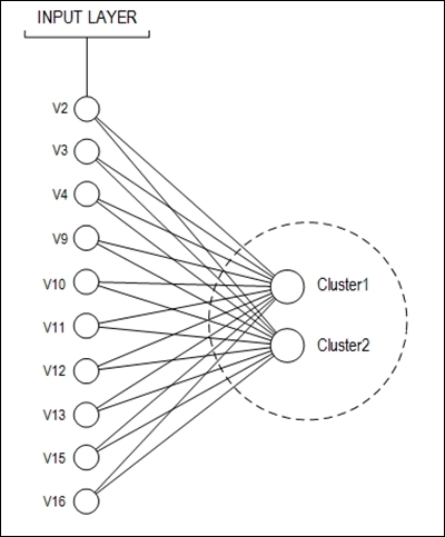
The number of examples stored is 690, but 37 of them have missing values. These 37 records were discarded. Therefore, 653 examples were used to train and test the neural network. The dataset division was made as follows:

The Kohonen training algorithm to cluster similar behavior depends on some parameters, such as the following:

It is important to note that the Kohonen training algorithm is unsupervised. So, this algorithm is used when the output is not known. In the card example, there are output values in the dataset and they will be used here only to attest clustering.

In this specific case, because the output is known, as classification, the clustering quality may be attested as follows:

In a Java project, the calculations of these values are done through the Classification class, previously developed in Chapter 6, Classifying Disease Diagnosis.

It is a good practice to perform many experiments to try to find the best neural net for clustering customer profiles. Ten different experiments will be conducted, and the quality rates will be analyzed for each, as mentioned earlier. The following table summarizes the strategy that will be followed:

The Card class was created to run each experiment. Regarding the training, we applied the Euclidian distance, as previously explained in Chapter 4, Self-Organizing Maps.

The following piece of code shows a bit of its implementation:

    Data cardDataInput = new Data("data", "card_inputs_training.csv");
    
    Data cardDataInputTestRNA  = new Data("data", "card_inputs_test.csv");
    Data cardDataOutputTestRNA = new Data("data", "card_output_test.csv");
  
    NormalizationTypesENUM NORMALIZATION_TYPE = Data.NormalizationTypesENUM.MAX_MIN;
  
  try {
    double[][] matrixInput = cardDataInput.rawData2Matrix( cardDataInput );
    
    double[][] matrixInputTestRNA = cardDataInput.rawData2Matrix( cardDataInputTestRNA );
    
    double[][] matrixOutput = cardDataInput.rawData2Matrix( cardDataOutputTestRNA );
    
    double[][] matrixInputNorm = cardDataInput.normalize(matrixInput, NORMALIZATION_TYPE);
    
    double[][] matrixInputTestRNANorm = cardDataInput.normalize(matrixInputTestRNA, NORMALIZATION_TYPE);
    
    NeuralNet n1 = new NeuralNet();
    n1 = n1.initNet(10, 0, 0, 2);
    
    n1.setTrainSet( matrixInputNorm );
    
    n1.setValidationSet( matrixInputTestRNANorm );
    n1.setRealMatrixOutputSet( matrixOutput );
    
    n1.setMaxEpochs(100);
    n1.setLearningRate(0.1);
    n1.setTrainType(TrainingTypesENUM.KOHONEN);
    n1.setKohonenCaseStudy( KohonenCaseStudyENUM.CARD );
    
    NeuralNet n1Trained = new NeuralNet();
    
    n1Trained = n1.trainNet( n1 );
    
    System.out.println();
    System.out.println("---------KOHONEN TEST---------");

    ArrayList<double[][]> listOfArraysToJoin = new ArrayList<double[][]>();
    
    double[][] matrixReal = n1Trained.getRealMatrixOutputSet();
    double[][] matrixEstimated = n1Trained.netValidation(n1Trained);
    
    listOfArraysToJoin.add( matrixReal );
    litOfArraysToJoin.add( matrixEstimated );
    
    double[][] matrixOutputsJoined = new Data().joinArrays(listOfArraysToJoin);
    
    //CONFUSION MATRIX
    Classification classif = new Classification();
    
    double[][] confusionMatrix = classif.calculateConfusionMatrix(-1.0, matrixOutputsJoined);
    classif.printConfusionMatrix(confusionMatrix);
    
    //SENSITIVITY
    System.out.println("SENSITIVITY = " + classif.calculateSensitivity(confusionMatrix));
    
    //SPECIFICITY
    System.out.println("SPECIFICITY = " + classif.calculateSpecificity(confusionMatrix));

    //ACCURACY
    System.out.println("ACCURACY    = " + classif.calculateAccuracy(confusionMatrix));
    
  } catch (IOException e) {
    e.printStackTrace();
  }

After running each experiment using the Card class and saving the accuracy rates, it is possible to observe that experiments 1 and 6 have the same accuracy. Data from the first experiment was normalized with the MIN_MAX method and data from the second experiment with MAX_MIN_EQUALIZED.

The following table displays the confusion matrix, sensitivity, and specificity of experiments 1 and 6. Again, please note that it is possible to observe the equivalence between the neural nets in both experiments. Only 6 patterns from 70 (less than 10%) could not be clustered correctly.

31.0 |  2.0
 4.0 | 33.0

31.0 |  2.0
 4.0 | 33.0