
Now, let's take a look at two examples of applications of these simple neural network architectures.
To facilitate understanding about perceptron, let's consider a basic warning system. It is based in AND logic. There are two sensors, and the rules of warning are as follows:
- If both or one of them is disabled, the warning is trigged
- If both are enabled, the warning is not trigged
The following figure shows the basic warning system:

To encode the problem, inputs are represented as follows. 0 means disabled, and 1 means enabled. Output is represented as follows. 0 means enabled, and 1 means disabled. The following table summarizes this:
|
Sample |
Sensor 1 |
Sensor 2 |
Alarm |
|---|---|---|---|
|
1 |
0 |
0 |
0 |
|
2 |
0 |
1 |
0 |
|
3 |
1 |
0 |
0 |
|
4 |
1 |
1 |
1 |
The Basic warning system figure illustrates how neurons and layers must be organized to solve this problem. It is the architecture of the neural net:

Now, let's use the class previously cited. Two methods have been created in the test class: testPerceptron() and testAdaline(). Let's analyze the first one:
private void testPerceptron() {
  NeuralNet testNet = new NeuralNet();

  testNet = testNet.initNet(2, 0, 0, 1);

  System.out.println("---------PERCEPTRON INIT NET---------");

  testNet.printNet(testNet);

  NeuralNet trainedNet = new NeuralNet();

  // first column has BIAS
  testNet.setTrainSet(new double[][] { { 1.0, 0.0, 0.0 },
    { 1.0, 0.0, 1.0 }, { 1.0, 1.0, 0.0 }, { 1.0, 1.0, 1.0 } });
  testNet.setRealOutputSet(new double[] { 0.0, 0.0, 0.0, 1.0 });
  testNet.setMaxEpochs(10);
  testNet.setTargetError(0.002);
  testNet.setLearningRate(1.0);
  testNet.setTrainType(TrainingTypesENUM.PERCEPTRON);
  testNet.setActivationFnc(ActivationFncENUM.STEP);

  trainedNet = testNet.trainNet(testNet);

  System.out.println();
  System.out.println("---------PERCEPTRON TRAINED NET---------");

  testNet.printNet(trainedNet);

  System.out.println();
  System.out.println("---------PERCEPTRON PRINT RESULT---------");

  testNet.printTrainedNetResult(trainedNet);

}
First, an object of the NeuralNet class is created. After that, this object is used to initialize the neural net with two neurons in the input layer, none in the hidden layer, and one neuron in the output layer. Then, a message and the untrained neural net are shown on the screen. Another object of the NeuralNet class is created and represents the trained neural net. After that, the testNet object is set with the training input dataset (the first column has bias values), training output dataset, maximum number of epochs, target error, learning rate, training type (perceptron), and activation function (step). Then, the trainNet method is called to train the neural net. To finalize, the perceptron-trained net results are printed. These results are shown in the following screenshot:

---------PERCEPTRON INIT NET---------
### INPUT LAYER ###
Neuron #1:
Input Weights:
[0.179227246819473]
Neuron #2:
Input Weights:
[0.927776315380873]
Neuron #3:
Input Weights:
[0.7639255282026901]

### OUTPUT LAYER ###
Neuron #1:
Output Weights:
[0.7352957201253741]

---------PERCEPTRON TRAINED NET---------
### INPUT LAYER ###
Neuron #1:
Input Weights:
[-2.820772753180527]
Neuron #2:
Input Weights:
[1.9277763153808731]
Neuron #3:
Input Weights:
[1.76392552820269]

### OUTPUT LAYER ###
Neuron #1:
Output Weights:
[0.7352957201253741]

---------PERCEPTRON PRINT RESULT---------
1.0  0.0  0.0   NET OUTPUT: 0.0   REAL OUTPUT: 0.0   ERROR: 0.0
1.0  0.0  1.0   NET OUTPUT: 0.0   REAL OUTPUT: 0.0   ERROR: 0.0
1.0  1.0  0.0   NET OUTPUT: 0.0   REAL OUTPUT: 0.0   ERROR: 0.0
1.0  1.0  1.0   NET OUTPUT: 1.0   REAL OUTPUT: 1.0   ERROR: 0.0
According to the results, it is possible to check whether the weights changed and conclude that the neural net learned how to classify when an alarm should be enabled or not. Reminder: The acquired knowledge belongs inside the weights [-2.820772753180527], [1.9277763153808731], and [1.76392552820269]. Besides, as the neurons are initialized with pseudo-random values, each time this code is run, the results change.
To demonstrate the adaline algorithm, let us imagine that a small part of a city has an avenue and three streets lead to this avenue. In this avenue, there are many accidents and heavy traffic. Assume that the government traffic department has decided to develop a forecasting and warning system. This system aims to anticipate traffic jams, warning drivers and taking the necessary measures to reduce the incurred losses, as demonstrated in the following figure:
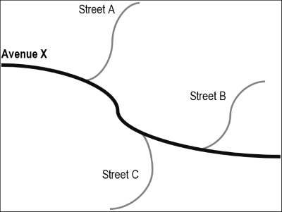
To develop the system, information is collected for every street and avenue for a week: the number of cars that travel on these routes per minute, as shown in the following table:
|
Sample |
Street A (cars/minute) |
Street B (cars/minute) |
Street C (cars/minute) |
Avenue (cars/minute) |
|---|---|---|---|---|
|
1 |
0.98 |
0.94 |
0.95 |
0.80 |
|
2 |
0.60 |
0.60 |
0.85 |
0.59 |
|
3 |
0.35 |
0.15 |
0.15 |
0.23 |
|
4 |
0.25 |
0.30 |
0.98 |
0.45 |
|
5 |
0.75 |
0.85 |
0.91 |
0.74 |
|
6 |
0.43 |
0.57 |
0.87 |
0.63 |
|
7 |
0.05 |
0.06 |
0.01 |
0.10 |
Then, the architecture of a neural net to solve this problem is designed as shown in the following figure:

Next, let's analyze the second test method named testAdaline(). It is as follows:
private void testAdaline() {

  NeuralNet testNet = new NeuralNet();

  testNet = testNet.initNet(3, 0, 0, 1);

  System.out.println("---------ADALINE INIT NET---------");

  testNet.printNet(testNet);

  NeuralNet trainedNet = new NeuralNet();

  // first column has BIAS

  testNet.setTrainSet(new double[][] { { 1.0, 0.98, 0.94, 0.95 },
      { 1.0, 0.60, 0.60, 0.85 }, { 1.0, 0.35, 0.15, 0.15 },
      { 1.0, 0.25, 0.30, 0.98 }, { 1.0, 0.75, 0.85, 0.91 },
      { 1.0, 0.43, 0.57, 0.87 }, { 1.0, 0.05, 0.06, 0.01 } });
  testNet.setRealOutputSet(new double[] { 0.80, 0.59, 0.23, 0.45, 0.74, 0.63, 0.10 });
  testNet.setMaxEpochs(10);
  testNet.setTargetError(0.0001);
  testNet.setLearningRate(0.5);
  testNet.setTrainType(TrainingTypesENUM.ADALINE);
  testNet.setActivationFnc(ActivationFncENUM.LINEAR);

  trainedNet = new NeuralNet();
  trainedNet = testNet.trainNet(testNet);

  System.out.println();
  System.out.println("---------ADALINE TRAINED NET---------");

  testNet.printNet(trainedNet);

  System.out.println();
  System.out.println("---------ADALINE PRINT RESULT---------");

  testNet.printTrainedNetResult(trainedNet);

  System.out.println();
  System.out.println("---------ADALINE MSE BY EPOCH---------");
  System.out.println( Arrays.deepToString( trainedNet.getListOfMSE().toArray() ).replace(" ", "
") );

}
The adaline test logic is very similar to perceptron's. The parameters that differ are as follows. Three neurons in the input layer, training dataset, output dataset, training type sets such as adaline, and activation function sets such as Linear. To finalize, adaline-trained net results and the adaline MSE list are printed. These results are shown in the following figure:

The complete results are displayed via following code:
---------ADALINE INIT NET---------
### INPUT LAYER ###
Neuron #1:
Input Weights:
[0.39748670958336774]
Neuron #2:
Input Weights:
[0.0018141925587737973]
Neuron #3:
Input Weights:
[0.3705005221910509]
Neuron #4:
Input Weights:
[0.20624007274978795]

### OUTPUT LAYER ###
Neuron #1:
Output Weights:
[0.16125863508860827]

---------ADALINE TRAINED NET---------
### INPUT LAYER ###
Neuron #1:
Input Weights:
[0.08239521813153253]
Neuron #2:
Input Weights:
[0.08060471820877586]
Neuron #3:
Input Weights:
[0.4793193652720801]
Neuron #4:
Input Weights:
[0.259894055603035]

### OUTPUT LAYER ###
Neuron #1:
Output Weights:
[0.16125863508860827]

---------ADALINE PRINT RESULT---------
1.0    0.98  0.94  0.95  NET OUTPUT: 0.85884   REAL OUTPUT: 0.8  ERROR: 0.05884739815477136
1.0    0.6    0.6    0.85  NET OUTPUT: 0.63925  REAL OUTPUT: 0.59
ERROR: 0.04925961548262592
1.0    0.35  0.15  0.15  NET OUTPUT: 0.22148  REAL OUTPUT: 0.23 ERROR: -0.008511117364128656
1.0    0.25  0.3    0.98  NET OUTPUT: 0.50103  REAL OUTPUT: 0.45 ERROR: 0.05103838175632486
1.0    0.75  0.85  0.91  NET OUTPUT: 0.78677   REAL OUTPUT: 0.74 ERROR: 0.046773807868144446
1.0    0.43  0.57  0.87  NET OUTPUT: 0.61637   REAL OUTPUT: 0.63 ERROR: -0.013624886458967755
1.0    0.05  0.06  0.01  NET OUTPUT: 0.11778  REAL OUTPUT: 0.1  ERROR: 0.017783556514326462

---------ADALINE MSE BY EPOCH---------
[0.04647154331286084,
0.018478851884998992,
0.008340477769290564,
0.004405551259806042,
0.0027480838150394362,
0.0019914963464723553,
0.0016222114177244264,
0.00143318844904685,
0.0013337070214879325,
0.001280852868781586]
One more time, according to the abovementioned results, it is possible to conclude that the neural net learned to predict traffic jams in a specific area. This can be proven by changing weights and by the MSE list. Look at the graphic plotted using the MSE data in the following figure. It is easy to note that the MSE decreases as the number of epochs increases.
