This chapter familiarizes you with SAS Enterprise Miner’s Variable Selection and Transform Variables nodes, which are essential for building predictive models. Since variable selection can also be done by the Variable Clustering and Decision Tree nodes, I have included some illustrations in this section of how to use these two nodes as well. Let us start with the Variable Selection node.

The Variable Selection node is useful when you want to make an initial selection of inputs or eliminate irrelevant inputs. It can also help identify non-linear relationships between the inputs and the target.

Unlike the Variable Selection node, the Variable Clustering node selects inputs without reference to the target variable. It is used primarily to identify groups (called clusters) of input variables that are similar looking and then to either select a representative variable from each cluster or create a new variable that is a linear combination of the inputs in a cluster. Replacing the variables in a cluster by the single variable that was selected or created to represent that cluster reduces the number of inputs and thereby reduces the severity of collinearity of the inputs in the estimation of the models.

The Decision Tree node can also be used for selecting important inputs. The inputs selected by the Decision Tree node are the inputs that contribute to the segmentation of the data set into homogeneous groups. The Decision Tree node is sometimes used after making an initial selection of inputs using the Variable Selection node.

The Transform Variables node provides a wide variety of transformations that can be applied to the inputs for improving the precision of the predictive models.

3.2 Variable Selection

In predictive modeling and data mining, we are often confronted with a large number of inputs (explanatory variables). The number of potential inputs to choose from may be 2000 or higher. Some of these inputs may not have any relation to the target. An initial screening can eliminate irrelevant variables and keep the number of inputs to a manageable size. A final selection can then be made from the remaining variables using either a stepwise regression or a decision tree.

The Variable Selection node performs the initial selection as well as a final variable selection. This section describes how the Variable Selection node handles interval and nominal inputs, as well as the selection criteria for categorical and continuous targets. The discussion focuses on four common situations (Cases 1–6):

• Case 1: The target is continuous (interval-scaled) and the inputs are numeric, consisting of interval-scaled variables.

• Case 2: The target is continuous and the inputs are categorical and nominal-scaled (These are sometimes referred to as class variables).

• Case 3: The target is binary and the inputs are numeric interval-scaled.

• Case 4: The target is binary and the inputs are categorical and nominal-scaled.

• Case 5: If the target is continuous and inputs are mixed, you have to specify how you want the Variables Selection node to handle categorical variables and continuous variables by appropriate property settings. The options considered in Case 1 and Case 2 are available even if you have mixed inputs. I did not include explicit examples for this case in this section because most of the examples included in subsequent chapters are with mixed inputs.

• Case 6: If the target is binary and inputs are mixed, you have to specify how you want the Variables Selection node to handle categorical variables and continuous variables by appropriate property settings. The options considered in Case 3 and Case 4 are available even if you have mixed inputs.

To focus on how each case is handled, use separate data sets for illustration purposes. In addition, to keep the discussion general, I indicate all numeric inputs as NVAR1, NVAR2, etc., and all nominal (character) inputs as CVAR1, CVAR2, etc.

Here are some examples of a continuous target:

• change in savings deposits of a hypothetical bank after a rate change

• customer’s asset value obtained from a survey of a brokerage company

• loss frequency of an auto insurance company

All the data I use here is simulated, so it does not refer to any real bank or company.

The binary target used in Case 3 and Case 4 represents a response to a direct mail campaign by a hypothetical auto insurance company. The binary target, as its name suggests, takes only two values—response (represented by 1), and no response (represented by 0).

In SAS Enterprise Miner, both ordinal and nominal inputs are treated as class variables.

3.2.1 Continuous Target with Numeric Interval-scaled Inputs (Case 1)

In this example, a hypothetical bank wants to measure the effect of a promotion that involves an increase in the interest rate offered on savings deposits in the bank. The target variable, called DEPV in the modeling data set, is the change in a customer’s deposits in response to the increase.

When the target is continuous (interval-scaled), the Variable Selection node uses R-Square as the default criterion of selection. For each interval-scaled input, the Variable Selection node calculates two measures of correlation between each input and the target. One is the R-Square between the target and the original input. The other is the R-Square between the target and the binned version of the input variable. The binned variable is a categorical variable created by the Variable Selection node from each continuous (interval-scaled) input. The levels (categories) of this categorical variable are the bins. In SAS Enterprise Miner, this binned variable is referred to as an AOV16 variable. The number of levels or categories of the binned variable (AOV16) is at most 16, corresponding to 16 intervals that are equal in width. This does not mean that the number of records in each bin is equal.

In general I recommend using AOV16 variables along with original variables and let the Regression node select the best one. If both are selected, you can use them both.

To get a better picture of these binned variables, let us take an example. Suppose we are binning the AGE variable, and it takes on values from 18–81. The first bin includes all individuals with ages 18–21, the second with ages 22–25, and so on. If there are no cases in a given bin, that bin is automatically eliminated, and the number of bins will be fewer than 16. The binned variable from AGE is called AOV16_AGE. The binned variable for INCOME is called AOV16_INCOME, and so on.

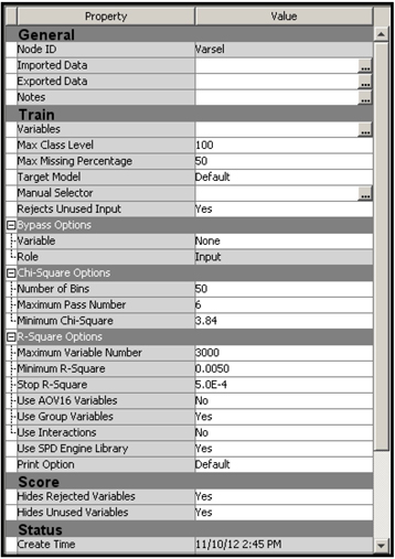
For this demonstration, I created a data source by selecting Advanced for the Metadata Advisor Option. Then I customized the properties, as shown in Display 3.1.

Display 3.1

The SAS data set used in the data source in this example is NUMERI_NTARG_B. The settings shown in Display 3.1 resulted in the following metadata.

Display 3.2

You can see that there are 227 interval scaled inputs and one binary input.

The Variable Selection node created 227 binned variables (AOV16 variables) from the interval-scaled variables, and then included all 455 variables in the selection process. At the end of the variable selection process, the Variable Selection node selected two original variables, NVAR133 and NVAR239, and three binned variables, AOV16_NVAR133, AOV16_NVAR049, and AOV16_NVAR239.

The following is a description of the variables that were selected.

NVAR133		average balance in the customer’s checking account for the 12-month period prior to the promotional increase in the interest rate at the hypothetical bank.
NVAR049		number of transactions during the past 12 months by the customer.
NVAR239		other deposit balance 3 months prior to the promotional rate change.

Note that variables NVAR133 and NVAR239 are selected in both their original form and in their binned form. As discussed in Chapter 2, only AOV16 variables are passed to the next node if you set the Use AOV16 Variables property to Yes. Because the Use AOV16 Variables property to Yes in this example, NVAR133 and NVAR239 are not passed to the next node as inputs. If you set the Hide Rejected Variables property (in the Score section of the Properties panel) to No, you can see the selected AOV16 variables and all the original variables in the list of variables passed to the successor node.

As we discussed in Chapter 2, Section 2.8.6.1, the R-Square method uses a two-step selection procedure. In the first step, a preliminary selection is made, based on Minimum R-Square. For the original variables, the R-Square is calculated from a regression of the target on each input; for the binned variables, it is calculated from a one-way Analysis of Variance (ANOVA).

The default value of the Minimum R-Square property is 0.005, but you can set this property to a different value. The inputs that have R-Square values above the lower bound set by the Minimum R-Square property are included in the second step of the variable selection process.

In the second step, a sequential forward selection process is used. This process starts by selecting the input variable that has the highest correlation coefficient with the target. A regression equation (model) is estimated with the selected input. At each successive step of the sequence, an additional input variable that provides the largest incremental contribution to the Model R-Square is added to the regression. If the lower bound for the incremental contribution to the Model R-Square is reached, the selection process stops. You can specify the lower bound for the incremental contribution to the Model R-Square by setting the Stop R-Square property to the desired value.

In this example, the Minimum R-Square property is set to 0.05 and the Stop R-Square property is set to 0.005. Ninety-two variables, some original and some binned, were selected in the first step and, of these, only five variables were selected in the second step.

The smaller the values to which Minimum R-Square and Stop R-Square properties are set, the larger the number of variables passed to the next node with the role of Input. Letting more variables into the next node makes more sense if there is a Decision Tree or Regression node downstream, as both these nodes can themselves perform rigorous methods of selection. Variable selection is automatic in the Decision Tree node but needs to be explicitly specified for the Regression node.

To use the Variable Selection node for preliminary variable selection only, set the minimum for the Stop R-Square property to a very low value such as 0.00001. This, in effect, bypasses Step 2 of the variable selection process, which is okay since Step 2 can always be done in the Decision Tree or Regression node.

The R-Square for the original raw inputs captures the linear relationship between the target and the original input, while the R-Square between a binned (AOV16) variable and the target captures the non-linear relationship. In our example, NVAR049 was not selected in its original form, but the binned version of it (AOV16_NVAR049) was selected. By plotting the target mean for each bin against the binned variable, you can see whether a non-linear relationship exists between the input and the target.

In the following pages, I show how to set up the properties of the Variable Selection node in SAS Enterprise Miner 12.1. Display 3.3 shows the process flow for the variable selection.

Display 3.3

The first tool in the process flow is the Input Data node, which reads the SAS modeling data set. The data set is then partitioned into Training, Validation, and Test data sets. The partitioning is done in such a way that 50% of the observations are allocated to Training, 30% to Validation, and 20% to Test. The Variable Selection node selects variables using only the Training data set. The selected variables are then passed to a Regression node, with the role of Input.

The selection criterion is specified by setting the Target Model property. Display 3.4 shows the properties panel of the Variable Selection node. In the case of a continuous target variable, only the R-Square method is available. When the Variable Selection node detects that the target is continuous, it selects the R-Square method.

Display 3.4

Because Use AOV16 Variables and Use Group Variables are both set to Yes, the AOV16 variables are created and passed to the next node, and all class variables are grouped (their levels collapsed). The Variable Selection node considers both the original and AOV16 variables in the two-step selection process, but only the selected AOV16 variables are assigned the role of Input and passed to the next node. If you also want to see the all the original inputs along with the selected AOV16 variables in the successor node, you should set the Hides Rejected Variables property in the Score section to No.

Output 3.1 shows a section of the output window in the Results window of the Variable Selection node. The output shows the variables selected in Step 1.

Output 3.1

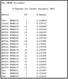
Output 3.1 (continued)

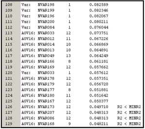
A number of variables have met the Minimum R-Square criterion in the preliminary variable selection (Step 1). Those that have an R-Square below the minimum threshold are not included in Step 2 of the variable selection process.

In Step 2, all the variables that are selected in Step 1 are subjected to a sequential forward regression selection process, as discussed before. In the second step, only a handful of variables met the Stop R-Square criterion, as can be seen from Output 3.2. This output contains a table taken from the output window in the Results window of the Variable Selection node.

Output 3.2

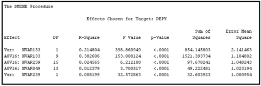
The variables NVAR133 and NVAR239 are selected both in their original form and in their binned forms. All other continuous inputs were selected in only their binned forms. Although many variables were selected in the preliminary variables assessment (Step 1), most of them did not meet the Stop R-Square criterion used in Step 2.

The next node in the process flow is the Regression node. I right-clicked on it and selected Update so that the path is updated. This means that the variables selected by the Variable Selection node are now passed to the Regression node with the role of Input. To verify this, I click located to the right of the Variables property of the Regression node. The Variables window opens, as shown in Display 3.5.

Display 3.5

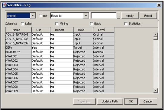
At the top of this window, the selected AOV16 variables are listed. In the Role column, the variables are given the role of Input. To see the role assigned to the variables NVAR133 and NVAR239, scroll down the Variables window. As you scroll, NVAR133 becomes visible. Scroll further to show NVAR239. Both these variables have the role Rejected, despite the fact that they were selected by the Variable Selection node. This is because I set the Use AOV16 Variables property to Yes in the Variable Selection node. Note also that, as Output 3.1 and Output 3.2 show, AOV16_NVAR133 and AOV16_NVAR239 have met both the Minimum R-Square and Stop R-Square criteria and hence are given the role of Input in the Regression node.

3.2.2 Continuous Target with Nominal-Categorical Inputs (Case 2)

The target variable here is the same as in Case 1, and all the inputs are nominal-scaled categorical.¹

Display 3.6 shows the process flow diagram created for demonstrating Case 2.

Display 3.6

In the case of nominal-scaled categorical inputs with a continuous target, R-Square is calculated using one-way ANOVA. Here you have the option of using either the original or the grouped variables. I decided to use only grouped class variables. If a variable cannot be grouped, it is still included in the selection process. Hence, I have set the Use Group Variables property to Yes in the Properties panel (Display 3.7). I made this choice because some of the class variables have too many categories. The term grouped variables refers to those variables whose categories (levels) are collapsed or combined. For example, suppose there is a categorical (nominal) variable called LIFESTYLE, which indicates the lifestyle of the customer. It can take values such as Urban Dweller, Foreign Traveler, etc. If the variable LIFESTYLE has 100 levels or categories, it can be collapsed to fewer levels or categories by setting the Group Variables property to Yes.

Following are descriptions of some of the nominal-scaled class inputs in my example data set:

CVR14		Customer segment, based on the value of the customer, where value is based on factors such as interest revenue generated by the customer. This takes only two values: High or Low.
CVAR03		A segment, based on the type of accounts held by the customer.
CVR13		A variable indicating whether the customer uses the Internet.
CVAR07		A variable indicating whether the customer contacts by phone.
CVAR06		A variable indicating whether the customer visits the branch frequently.
CVAR11		A variable indicating whether the customer holds multiple accounts.

Display 3.7

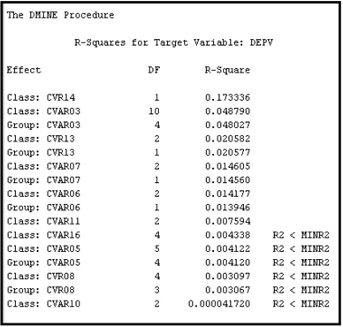
Output 3.3 shows the variables selected in Step 1 of the Variable Selection node.

Output 3.3

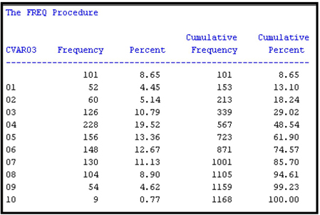
To see how SAS Enterprise Miner groups or collapses categorical variables, let us consider the nominal scale variable CVAR03. By using PROC FREQ in the SAS Code node, we can see that the nominal-scaled variable CVAR03 has 11 categories, including the “missing” or unlabeled category, as shown in Output 3.4.

Output 3.4

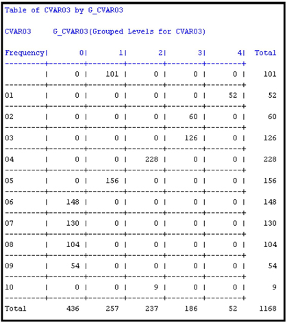
The Variable Selection node created a new variable called G_CVAR03 by collapsing the eleven categories of CVAR03 into five categories. Using PROC FREQ again, we can see the frequency distribution of the categories of G_CVAR03, which is shown in Output 3.5. Output 3.5A shows a cross tabulation of CVAR03 by G_CVAR03.

Output 3.5

Output 3.5A

The SAS code that generated Outputs 3.4, 3.5, and 3.5A is shown below:

Display 3.8 shows which categories of CVAR03 are grouped (collapsed) to create the variable G_CVAR03.

Display 3.8

The grouping procedure that SAS Enterprise Miner uses in collapsing the categories of a class variable can be illustrated by a simple example. Suppose a class variable has five categories: A, B, C, D, and E. For each level, the mean of the target for the records in that level is calculated. In the case of a binary target, if I represent a response by 1 and non-response by 0, then the target mean for a given level of an input variable is the proportion of responders within that level. The levels (categories) are then sorted in descending order by their target means. That is, the category that has the highest mean for the target becomes the first category, the one with the next highest target mean is second, and so on. Suppose this ordering resulted in this ranking: C, E, D, A, and B. Then the procedure combines the categories starting from the top. First it calculates the R-Square between the input and the target prior to grouping. Suppose the R-square is 0.20. Next, the procedure combines the categories C and E and recalculates the R-Square. Now the input has four categories instead of five, and the R-Square between the input and the target is now less than 0.20. If the reduction in R-Square is less than 5%, then C and E remain combined. A reduction of less than 5% in an R-Square of 0.20 means that the newly grouped input must have an R-square of at least 0.19 with the target. If not, C and E are not combined. Then an attempt is made to combine E and D using this same method, and so on. Output 3.3 shows the R-Square between the target and the original inputs before grouping (labeled Class) as well as the R-square between the target and the grouped version of the inputs (labeled Group).

The nominal-scaled variable CVAR03 has an R-Square of 0.048790 with the target before its categories are combined or grouped, and an R-Square of 0.048027 after collapsing the categories (grouping) from 11 to 5. The reduction in R-Square due to grouping is 0.000763 or 1.56%, which is less than 5%.

Both G_CVAR03 and CVAR03 met the R-Square criterion and were selected in Step 1. However, only the grouped variable is kept in the final Step 2 selection, as can be seen in Output 3.6. The R-Square shown in Output 3.6 is an incremental or sequential R-Square, as distinct from the bivariate R-Square (coefficient of determination) shown in Output 3.3.

Output 3.6

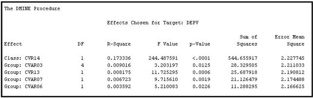
The first variable, CVR14, is a two-level class variable, and hence its levels are not collapsed (see Output 3.3, and note that no Group version of CVR14 appears). As before, the final selection is based on the stepwise forward selection procedure. The procedure starts with the best variable, i.e., the variable with the highest correlation, followed by the other variables according to their contribution to the improvement of the stepwise R-Square.

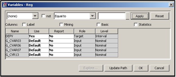
Next the Regression node is connected to the Variable Selection node. Display 3.9 shows the variables that are passed on to the Regression node with the role of Input.

Display 3.9

3.2.3 Binary Target with Numeric Interval-scaled Inputs (Case 3)

In this example, a hypothetical bank wants to cross-sell a mortgage refinance product. The bank sends mail to its existing customers. The target variable is response to the mail, taking the value of 1 for response and 0 for non-response.

The following is a description of some of the inputs in the data set used in this example.

NVAR004		credit card balance
NVAR014		auto loan balance
NVAR016		auto lease balance
NVAR030		mortgage loan balance
NVAR044		other loan balances
NVAR075		value of monthly transactions in checking and savings accounts
NVAR137		number of direct payments by the bank per month
NVAR148		available credit
NVAR187		number of investment-related transactions per month
NVAR193		percentage of households with children under age 10 in the block group
NVAR195		percentage of households living in rented homes in the block group
NVAR210		length of residence
NVAR286		age of the customer
NVAR315		number of products owned by the customer
NVAR318		number of teller-transactions per month

In the case of binary targets, inputs can be selected by using either the R-Square criterion, as in Case 1, or the Chi-Square criterion.

3.2.3.1 R-Square Criterion

When the target is binary then Chi-Square criterion is more appropriate than the R-square criterion especially if your goal is to estimate a logistic regression with the selected inputs. However, the continuous (interval-scaled inputs) have to be “binned” in order to calculate the Chi-Square statistics. This may be time consuming if there are many continuous inputs. Binning may also result in some loss of information. You can avoid binning the continuous variables if you use the R-Square criterion. In practice there is usually overlap between the variables selected under the Chi-Square and R-square criteria. So it is best to pass the union of the two sets of variables selected by these two methods to the next node (such as the Regression node or Decision Tree node) where further variable selection takes place.

When the R-Square criterion is used, the variable selection is similar to the case in which the target is continuous (Case 1). The target variable is treated like a continuous variable, and the R-Square with the target is computed for each original input and for each binned input (AOV16 variable.) Then the usual two-step procedure is followed: In the first step, an initial variable set is selected based on the Minimum R-Square criterion; in the second step, a sequential forward selection procedure is used to select variables from those selected in Step 1 on the basis of a Stop R-Square criterion. Inputs that meet both these criteria receive the role of Input in the subsequent modeling tool, such as the Regression node.

3.2.3.2 Chi-Square Criterion

The Chi-Square criterion can be used only when the target is binary. When the Chi-Square criterion is selected, the selection process does not have two distinct steps, as in the case of the R-square criterion. Instead, a tree is constructed. The inputs selected in the construction of the tree are passed to the next node with the assigned role of Input. In this example, there are 302 inputs, and the Variable Selection node selected 19 inputs. This selection is done by developing a tree based on the Chi-Square criterion, as explained below. A tree constructed using the Chi-Square criterion is sometimes called CHAID (Chi-Squared Automatic Interaction Detection).

The tree development proceeds as follows. First, the records of the data set are divided into two groups. Each group is further divided into two more groups, and so on. This process of dividing is called recursive partitioning. Each group created during the recursive partitioning is called a node. The nodes that are not divided further are called terminal nodes, or leaf nodes, or leaves of the tree. The nodes that are divided further are called intermediate nodes. The node with all the records of the data set is called the root node. All these nodes form the tree. Displays 3.10 and 3.11 show such a tree.

In order to split the records in a given node into two new nodes, the algorithm evaluates all inputs (302 in this example) one at a time, and finds the best split for each input. To find the best split for an interval input the algorithm first divides the input into intervals, or bins, of equal length. The number of bins into which the interval input is divided is determined by the value to which the Number of Bins property is set. The default value is 50. However, suppose you set it to 10 and the interval input to be binned is income, with values that range from $10,000 to $110,000 in the data set. In that case, the 10 equal intervals will be $10,000– $20,000, $20,000–$30,000, $30,000–$40,000...and $100,000–$110,000. Any node split based on this input will be partitioned at one of the split values of $20,000, $30,000, $40,000, etc. A 2x2 contingency table is created for each of these nine split values, and a Chi-Square statistic is computed for each split. In this example, there are nine Chi-Square values. The split value with the highest Chi-Square value is the best split based on the input income. Then the algorithm does a similar calculation to find the best split of the records on the basis of each of the other available inputs. After finding the best split for each input, the algorithm compares the Chi-Square values of all these best splits and picks the one that gives the highest Chi-Square value. It then splits the records into two nodes on the basis of the input that gave the best split. This process is repeated at each node. All those inputs that are selected in this process, i.e. those that are chosen to be the basis of the split at any node of the tree, are passed to the next node with the assigned role of Input.

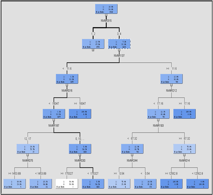
The tree generated by the Variable Selection node for our example data is shown in Displays 3.10 and 3.11. Display 3.10 shows the root node and the half of the tree. Display 3.11 shows the root node and the right half of the tree.

Display 3.10

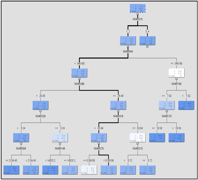
Display 3.11

Display 3.12 shows the relative importance of the selected variables.

Display 3.12

The variables that appear in Displays 3.10 and 3.11 are passed to the next node with the role of Input. You can verify this by first connecting a Regression node to the Variable Selection node, as shown in Display 3.13.

Display 3.13

Then, if you select the Regression node, update the path and click to the right of the Variables property in the Properties panel, a window appears displaying the inputs passed to the Regression node. This is shown in Display 3.14.

Display 3.14

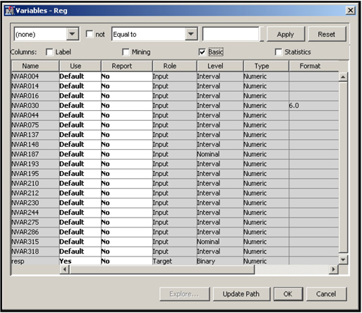
Display 3.14 shows that the role assigned to each of these selected variables is Input. Note that NVAR187 and NVAR315 are numeric, but are treated by SAS Enterprise Miner as nominal (see the column titled Level in Display 3.14) since each of them has fewer than 20 distinct values. NVAR187 has 13 distinct values, and NVAR315 has 7 distinct values.

Unlike the Decision Tree node, the Variable Selection node does not create dummy variables from the terminal nodes under the Chi-Square criterion. The Chi-Square criterion is discussed in more detail in Chapter 4 in the context of decision trees.

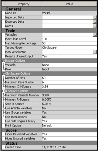
Display 3.15 shows the properties panel where the properties for the Chi-Square criterion are set.

Display 3.15

3.2.4 Binary Target with Nominal-scaled Categorical Inputs (Case 4)

In this case, the target variable is the same as in Case 3, and all the inputs are nominal-scaled categorical. You can use either the R-Square or Chi-Square criterion to select the variables. Here are descriptions of some of the nominal-scaled class inputs in the data set:

CVAR08		dwelling size code
CVAR11		income code
CVAR20		indicator of home ownership
CV30		demographic cluster
CVAR34		indicator of Internet banking
CVAR35		customer type
CVAR40		life cycle code
CVAR47		indicator of Internet usage

Display 3.16 shows the process flow used to demonstrate the examples in this section.

Display 3.16

3.2.4.1 R-Square Criterion

With the R-Square criterion, the selection procedure is similar to the procedure in Case 2 in which two steps are needed. I set the Target Model property to R-Square and ran the Variable Selection node. The variables selected in Step 1 are shown in Output 3.7.

Output 3.7

Output 3.8 shows the results of the forward selection process (Step 2).

Output 3.8

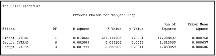
When you compare Outputs 3.7 and 3.8, you can see that the class variables CVAR40 and CVAR35 met the Minimum R-Square criterion in the first step in their original and grouped form. But in the second step, only the grouped variables survived. Display 3.17 shows the variables window of the next node, which is the Regression node.

Display 3.17

3.2.4.2 Chi-Square Criterion

Using the same data set, I selected the Chi-Square criterion by setting the value of the Target Model property to Chi-Square.

Display 3.18 shows the tree constructed by this method.

Display 3.18

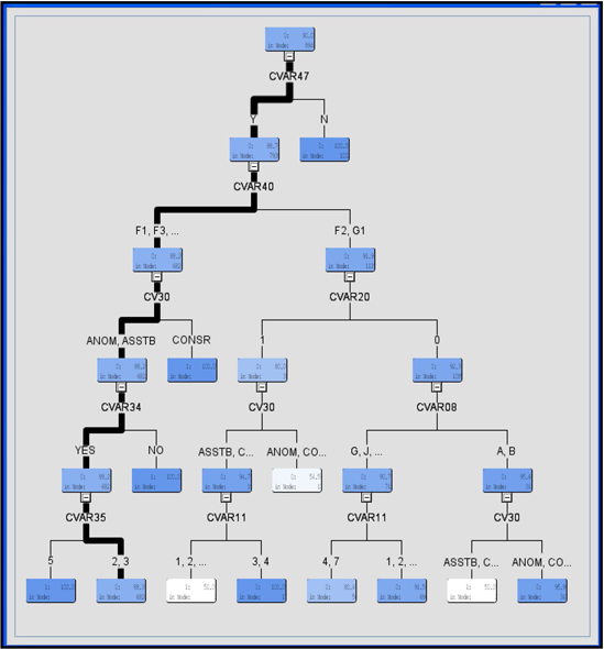
The names of the variables selected appear below the intermediate (non-terminal) nodes of the tree. Display 3.19 shows the variable importance.

Display 3.19

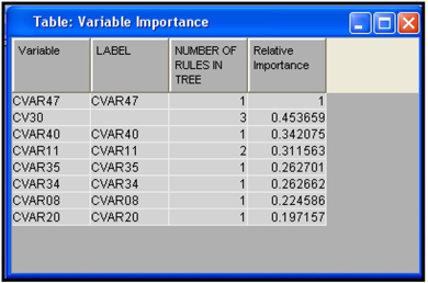
When you compare the variables in Display 3.19 with those in Outputs 3.7 and 3.8, you can see that CVAR47 emerges as the most important variable by both the R-Square and Chi-Square criteria. As you may recall, this variable is an indicator of Internet usage by the customer in the data set.

The variables in Display 3.19 are exported to the next node. In this example, the next node is the Regression node. Open its Variables window to see the same variables with the role of Input. The variables window of the Regression node is shown in Display 3.20.

Display 3.20

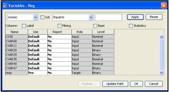
Eight variables were selected—those that produced the best splits in the development of the tree. The selected variables are given the role of Input in the Regression node.

3.3 Variable Selection Using the Variable Clustering Node

In this section, I show how the Variable Clustering node is used for variable (input) selection. The variable selection done by the Variable Clustering node differs from the variable selection done by the Variable Selection node. The Variable Selection node selects the inputs on the basis of the strength of their relationship with the target (dependent) variable, whereas the Variable Clustering node selects the variables without reference to the target variable. The Variable Clustering node first creates clusters of variables, by assigning variables that look similar to the same cluster. Then it selects one representative variable from each cluster. You can also ask for a linear combination of all variables in a cluster, instead of one representative variable from each cluster. The linear combination of the variables that the Variable Clustering node creates from each cluster is called the component of the cluster.

In Chapter 2 we discussed in detail how these clusters are created and how the components are calculated from the clusters. Whether you are using representative variables from the clusters or using the cluster components, you are in effect reducing the number of inputs substantially. In this section, I demonstrate both these methods of input reduction and develop a predictive model with the reduced set of inputs, and compare the resulting models. The model development and model comparison are discussed in detail in Chapters 4, 5, 6 and 7. I hope that the exercise in this section provides a preview of these tasks without causing confusion.

To do this demonstration, I constructed a modeling data set for a sample of 15,000 customers. The data set has 15,000 observations, one for each customer, and 85 columns, 84 of which refer to the inputs or explanatory variables and one of which refers to the target variable named Event. The Event variable shows whether the customer canceled (closed) his/her account during the 3-month observation window. The 84 inputs in the data set include variables that describe the customer’s behavior prior to the observation window, as well as other characteristics such as age and marital status of the customer. If the variable Event takes the value 1 for an account, it means that the account closed during the observation window (0 indicates that the account remained open). From past experience we know that the event (cancellation) rate is 2.4% per 3 months, but since the sample we are using is biased, it shows an event rate of around 16%.

We use the Variable Clustering node to create a number of clusters of inputs. In our example, we use the default settings for all of the properties of the Variable Clustering node—except the Variable Selection property, which we set first to Best Variables and then to Cluster Component.

The Best Variables setting selects one representative input from each cluster, while the Cluster Component setting selects the cluster component (a linear combination of the inputs in a given cluster) of each cluster.

The selected variables or cluster components are then passed to the Regression node, which estimates a logistic regression using the inputs passed to it and the target variable Event. Then we compare the logistic regressions estimated from these two methods of selection.

The Regression Node is discussed in detail in Chapter 6. Here I use it only to illustrate how the variables selected by the Variable Clustering node are passed to the next node and how they can be used in the next node.

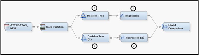
Display 3.21 shows the process flow for demonstrating variable selection by the Variable Clustering node.

Display 3.21

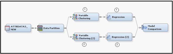
Display 3.21 shows both of the approaches to variable clustering that I want to demonstrate. In the first approach, shown in the upper segment of Display 3.21, I set the Variable Selection property to Best Variables. All other properties are set to their default values. The default value for the Include Class Variables property is No. With these settings, the Variable Clustering node creates clusters of variables, identifies the best variable in each cluster, and passes the best variable from each cluster on to the next node. (Recall from Chapter 2 that the best variable in any given cluster is the one that has the minimum 1-RSquare ratio.) Since the Include Class Variables property is set to No, all of the nominal (class) variables among the inputs are passed to the next node along with the best variables. If the Include Class Variables property is set to Yes instead, the variable clustering algorithm creates dummy variables for each category of each class variable and includes these dummy variables in the process of creating the clusters.

3.3.1 Selection of the Best Variable from Each Cluster

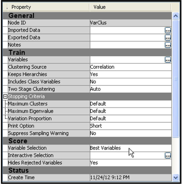
Display 3.22 shows the properties of the Variable Clustering node in the upper section of Display 3.21.

Display 3.22

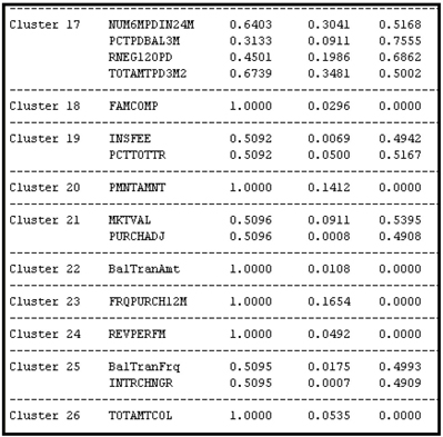
The clusters and the variables in each cluster can be seen in the output window of the Variable Clustering node, as shown in Output 3.9.

Output 3.9

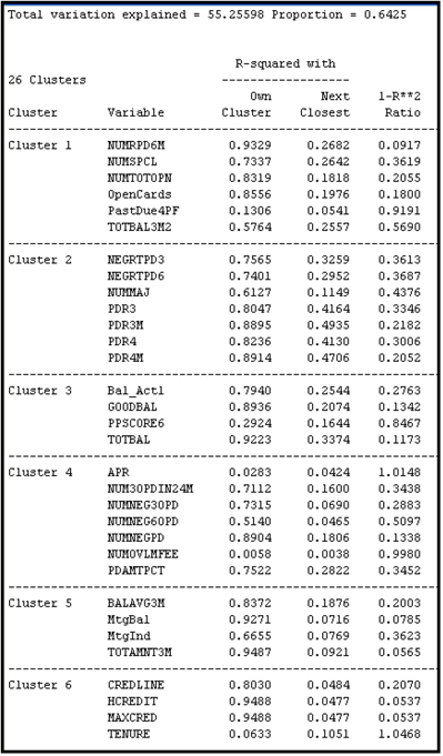
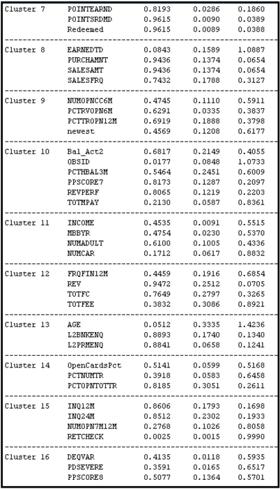
Output 3.9 (cont’d)

Display 3.23 shows the selected variables.

Display 3.23

Next we connect a Regression node to the Variable Clustering node in the upper section of Display 3.21. The variables shown in Display 3.23 and the nominal variables that were excluded from clustering are passed to the Regression node.

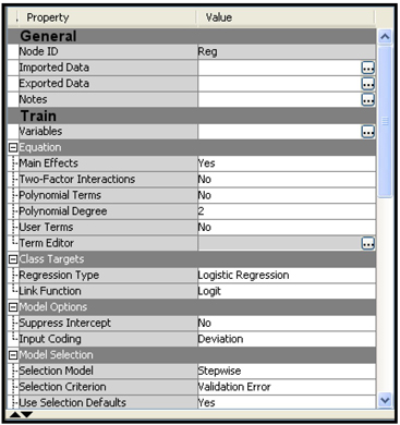
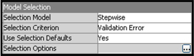
In the Regression node, we make a further selection of these variables by setting the Selection Model Property to Stepwise and the Selection Criterion property to Validation Error. With these settings, the Regression node tests all the variables passed to it and selects the variables to keep based on the Stepwise selection criterion. During this process of variable selection, the Regression node creates a number of models and selects the model that has the smallest error when applied to the Validation sample.

Display 3.24 shows the property settings of the Regression node shown in the upper segment of Display 21.

Display 3.24

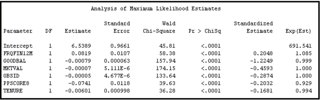
Output 3.10 shows the estimated logistic regression.

Output 3.10

The logistic regression presented in Output 3.10 is part of the output sub-window of the Results window. The inputs included in the logistic regression shown in Output 3.10 can be considered the best of the best because variables entered into the logistic regression were passed through two selection processes. The Variable Clustering node first selected the best interval-scaled input from each cluster and passed them to the Regression node along with all the nominal variables present in the data set. The Regression node then selected the best of these variables through the stepwise selection. Hence, the inputs included in the regression equation presented in Output 3.10 can be considered the best of the best in a statistical sense. In general, you should pay careful attention to the sign of the parameter estimates and make sure that they make business sense.

In order to help assess the regression equation, the Results window also produces a number of charts. You can use two charts described below to compare the logistic regressions estimated from the alternative variable selections that we have made. The first chart is called the Lift chart. In order to create the Lift chart, the Regression node first applies the model to a data set that contains all the inputs used in the estimated regression. Then, for each observation (customer), it uses the estimated regression coefficients and specification to calculate the probability that each customer will close his/her account or “attrit” (cancellation is sometimes referred to as attrition). Then, once this estimated probability of attrition is calculated for each customer, the Regression node sorts the data set in descending order of the calculated probabilities. That is, it ranks all the customers in the database by their probability to cancel their accounts, with those most likely to cancel at the top of the list. Then it divides the data set into 20 equal segments called Percentiles. Since the percentiles are created from the sorted data set based on the computed probabilities, the first percentile (called the top percentile) has the customers with the highest mean probability of cancellation. If the model is accurate, then the first percentile in this ranked list should also have the highest actual observed cancellation rate, where the cancellation rate is defined as the number of cancellations in a given percentile divided by the number of observations in the percentile. The Regression node calculates the observed cancellation rates for each of the 20 percentiles created as described above.

The lift in a given percentile is the actual observed cancellation rate in that percentile divided by the overall actual cancellation rate for the data set. Suppose the top percentile has an actual observed cancellation rate of 55.1% and the overall cancellation rate is 16%; the lift in the top percentile is 55.1/16, or 3.44. Similarly, if the actual observed cancellation rate is 30.67% in the second percentile, then the lift in the second percentile is 30.67/16.0, or 1.92. These lift numbers provide a good measure of the ability of the estimated model to predict which customers will cancel and which will not.

The Regression node calculates the lift for the Training and Validation data sets. The partition of the data into Training, Validation, and Test is done by the Data Partition node, which is the second node in the process flow diagram shown in Display 3.21.

In addition to calculating the lift for each percentile separately, the Regression node calculates the cumulative lift. The cumulative lift calculated above for the first percentile is 3.44. The cumulative lift at the second percentile is the combined lift of the first and second percentiles. The first and second percentiles together contain 10% of the observations in the data set. If the cancellation rate in the first and second percentiles together is 42.89%, then the cumulative lift at the second percentile is 42.89/16.0, or 2.68. If the cancellation rate for the first, second and third percentiles together is 37.63%, then the cumulative lift at the third percentile is 37.63/16.0, or 2.35. The cumulative lift is calculated for each of the 20 percentiles.

Output 3.11 shows the response rate (which is the cancellation rate or attrition rate in this example), cumulative response rate (cumulative cancellation rate), lift, cumulative lift, and other statistics calculated from the Training data set. Output 3.12 shows these statistics calculated from the Validation data set.

Output 3.11

Output 3.12

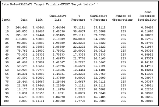
You can find Output 3.11 and 3.12 if you scroll down the output sub-window of the Results window of the Regression node shown in the upper part of Display 3.21.

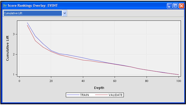
Display 3.25 shows the graphs of the cumulative lift provided by the model when it is applied to the Training data set (see Output 3.11) and to the Validation data set (see Output 3.12.) These charts show the predictive performance of the logistic regression that was based on the best variables selected from each cluster.

Display 3.25

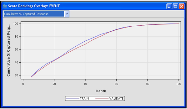
Another measure of the model’s power to discriminate between the bad (cancellations) and the good (no cancellation) is the Cumulative % Captured Response. The Cumulative % Captured Response at a given percentile is the percentage of observed cancellations (events) in that percentile and in all the preceding percentiles. In other words, it is the number of cancellations observed in that percentile and in all the preceding percentiles combined, divided by the total number of cancellations in the data set.

Display 3.26 shows the Cumulative Capture Rate by percentile from the training and validation data sets.

Display 3.26

By selecting Cumulative % Captured Response (see Display 3.26) chart in the Results window and clicking the table icon, you can see the table that shows the numbers behind the chart in Display 3.26. A partial view of this table is shown in Display 3.27.

Display 3.27

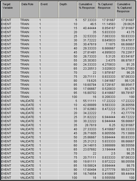
From the chart in Display 3.26 and the underlying table shown in Display 3.27, it is clear that 43.75% of all cancellations in the Training data set are in the top 20 percentiles, and 42.78% of all cancellations in the Validation data set are in the top 20 percentiles. When considering retention programs, you can apply this model to current customers and target only those customers in the top few percentiles, and still reach a large proportion of vulnerable customers, i.e., customers with a high probability of attrition.

3.3.2 Selecting the Cluster Components

In this section, we set the Variable Selection property of the Variable Clustering node (shown in the lower part of Display 3.21) to Cluster Component. We keep all the other property settings of the Variable Clustering node the same as they were in the Variable Clustering node example in section 3.3.1. Then we attach a Regression (2) node to the Variable Clustering (2) node, set its properties to the same values used for the Regression node in section 3.3.1, and then run the whole path.

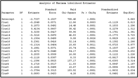
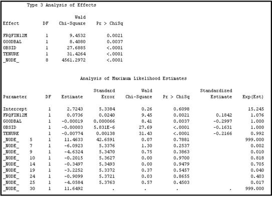
After running the Variable Clustering node, all the components (denoted by Clus1, Clus2…, Clus26) from the 26 clusters plus any nominal variables that were excluded from the clustering process were passed to the Regression node. The stepwise selection procedure of the Regression node resulted in the selection of a logistic regression equation with some of the cluster components, as can be seen in Output 3.13.

Output 3.13

In order to compare the two models, i.e. the model based on the Best Variables option and the model based on the Cluster Component option, a Model Comparison node is attached at the end of the process flow (see Display 3.21). When we run the Model Comparison node, it calculates the cumulative lifts and cumulative capture rates by percentile for both the models.

Display 3.28 shows the Cumulative Lift charts and Display 3.29 shows the Cumulative Capture Rates.

Display 3.28

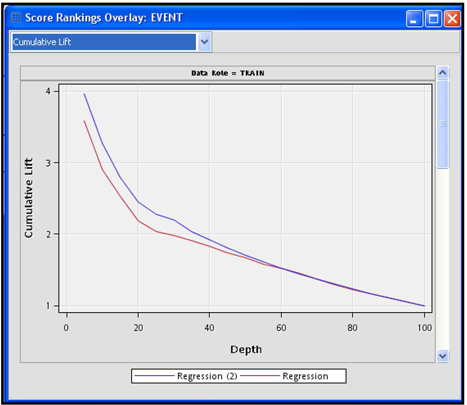
In Display 3.28, the line labeled Regression refers to the logistic regression based on the Best Variables selection, and Regression (2) refers to the logistic regression based on the cluster components. To make it easier, let us call the logistic regression based on the Best Variables option Model 1, and the logistic regression based on the Cluster Components option Model 2.

Display 3.29

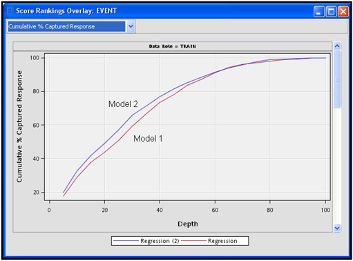
Display 3.29 shows that the cumulative capture rate of Model 2 is above that of Model 1 at each percentile. But the difference between these two models is very small. Since Model 1 uses actual inputs rather than the cluster components that were constructed from the actual inputs, it is easier to interpret the coefficients of Model 1 than those of Model 2.

3.4 Variable Selection Using the Decision Tree Node

In Section 3.3 we used the Variable Clustering node to select inputs by creating groups of inputs called clusters. In this section, we use the Decision Tree node to select the inputs which are most useful in creating groups of customers called segments or leaf nodes. The target variable played no role in variable clustering, whereas it plays an important role in the Decision Tree node.

When you have a very large number of variables, you can first eliminate obviously irrelevant variables using the Variable Selection node, and then use the Decision Tree node for further variable selection.

The Decision Tree node successively splits the observations in the data set into non-overlapping segments by assigning all observations with values for a certain inputs that fall within the same range to the same node of the tree. The ultimate segments that are created at the end of a series of successive splits are called leaf or terminal nodes. Each leaf node or segment is assigned a number. After the partitioning is completed, each observation in the data set belongs to one and only one segment or leaf node. The Decision Tree node creates a variable named _NODE_ that indicates to which leaf (or segment) an observation belongs. The variable _NODE_ is a categorical variable whose values are the leaf or segment numbers.

For creating the segments, the tree node uses the best variables. The inputs that provide good splits are selected. These selected variables are given the model role of Input and passed to the next node. The variables that were not used in the partitioning are assigned the model role of Rejected. The variable _NODE_ is also passed to the next SAS Enterprise Miner node. (Remember that the _NODE_ variable refers to the nodes of the decision tree that you have just estimated, not to the nodes of SAS Enterprise Miner.) You can use the _NODE_ variable as an additional input or use it only for identifying the segment.

In this section, I show how you can use the variables selected by the Decision Tree node in the next node, which is again the Regression node in this example. We develop two Logistic Regression models. In the first model, we use the variables selected by the Decision Tree node, but not the special variable _NODE_, as an input. This is Model A. In the second model, we use the special variable _NODE_ as in input, in addition to all the variables selected by the Decision Tree node. This is Model B. Then, as in Section 3.3, we compare these two models using the Model Comparison node.

Display 3.30 shows the process flow for this example. Model A is created by the sequence of nodes in the upper segment of Display 3.30, and Model B uses the nodes on the bottom.

Display 3.30

For Model A, the Leaf Role property of the Decision Tree node is set to Segment. This setting results in treating the variable _NODE_ as a segment variable (an identifier of the node), and not as a variable that can be used as an input in the subsequent nodes. The Regression node that follows the Decision Tree node will not use the variable _NODE_ as an input.

Output 3.14 shows the equation estimated without using the variable _NODE_ (Model A).

Output 3.14

For Model B, the Leaf Role property of the Decision Tree node is set to Input. This setting results in treating the variable _NODE_ as an input. The Regression node that follows the Decision Tree node will include the variable _NODE_ as a nominal variable in selecting variables and estimating the logistic regression equation.

Output 3.15 shows the equation estimated using the variable _NODE_ (Model B).

Output 3.15

In both models, the properties of the Regression nodes are set such that they make a further selection of variables from the sets of variables that are passed to them from the Decision Tree nodes that precede them. Each Regression node selects, from the sequence of models it creates in the Stepwise selection process, the model that has the smallest validation error. These settings for the properties are shown in Display 3.31.

Display 3.31

Display 3.32 shows the Captured % Response for both models.

Display 3.32

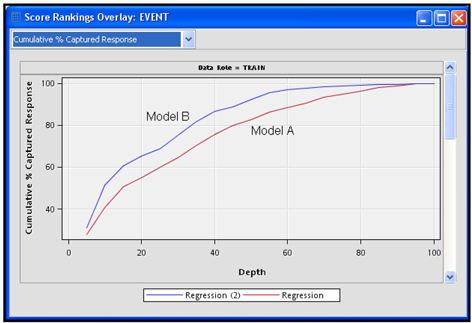
It appears that Model B, which makes use of the special variable _NODE_, is slightly better than Model A in the sense that the Cumulative %Captured Cancellations curve of Model B is higher than that for Model A.

3.5 Transformation of Variables

3.5.1 Transform Variables Node

The Transform Variables node can make a variety of transformations of interval-scaled variables. These were described in Section 2.9.6.1. In addition, there are two types of transformations for the categorical (class) variables.

• Group Rare Levels

• Dummy Indicators Transformation for the categories (see Section 2.9.6.2)

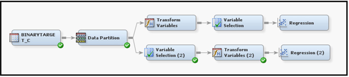
If you want to transform variables prior to variable selection, you can set up the path as Input Data node → Data Partition node → Transform Variables node → Variable Selection node, as shown in the upper path in Display 3.33. If you do not want to reject inputs on the basis of linear relationship alone, you can use this process to capture non-linear relationships between the inputs and the target. However, with large data sets this process may become quite tedious.

When there are a large number of inputs (2000 or more), it may be more practical to eliminate irrelevant variables first, and then define transformations on important variables only. The process flow for this is Input Data node → Data Partition node → Variable Selection node→ Transform Variables node (shown in the lower path of Display 3.33). This section examines the results of both of these sequences with alternative transformations using a small data set. The process flow shown in Display 3.33 does not include the Impute node, but in any given project you might need to use this node before applying transformations or selecting variables.

Display 3.33

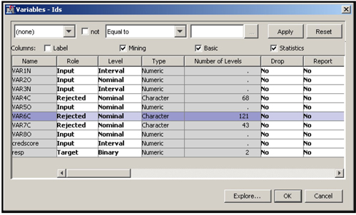
To demonstrate the transformations, I have selected a small number of inputs and the binary target RESP, which represents the response to a solicitation by a hypothetical bank. Here are these inputs, shown in Display 3.34:

VAR1N		number of on-line inquiries by the customer per month
VAR2O		number of ATM deposits during the past three months
VAR3N		number of ATM withdrawals during the past three months
VAR4C		lifestyle indicator
VAR5O		number of asset types
VAR6C		an indicator of wealth
VAR7C		life stage segment
VAR8O		total number of bank products owned by the customer
CREDSCORE		credit score
RESP		target variable; indicates response to an offer

Display 3.34

3.5.2 Transformation before Variable Selection

In the upper path of Display 3.33, the variables are transformed using the Transform Variables node and then passed to the Variable Selection node.

In the Transform Variables node, I selected the Maximum Normal transformation as the default method for all continuous variables by setting the Interval Inputs property to Maximum Normal. The node generates different power transformations of the variable and picks the transformation that transforms the input into a new variable whose distribution is closest to normal, bell-shaped, distribution. (Section 2.9.6.1 gives the details of this process). For class inputs, I selected the Dummy Indicators transformation by setting the Class Inputs property to Dummy Indicators.

This data set has three interval-scaled variables: VAR1N, VAR3N, and credscore. If a numeric variable has only a few values, then SAS Enterprise Miner sets its measurement level to Nominal if you select Advanced for the Metadata Advisor Option when you created the data source (see Displays 2.10 and 2.11). VAR2O, VAR5O, and VAR8O are numeric variables and are set to Nominal by SAS Enterprise Miner. For the variables set to interval-scaled, the node searches and finds the Maximum Normal, as I specified earlier. For the rest of the variables, which are now nominal scaled, it creates a dummy variable for each level. The transformed variables are then passed to the next node in the process flow. In this example, the Variable Selection node follows the Transform Variables node.

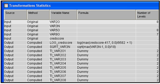
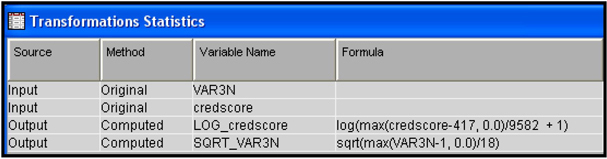
By running the Transform Variables node and opening the Results window, you can see the Transformation Statistics. Display 3.35 shows a partial view of the Transformation Statistics table.

Display 3.35

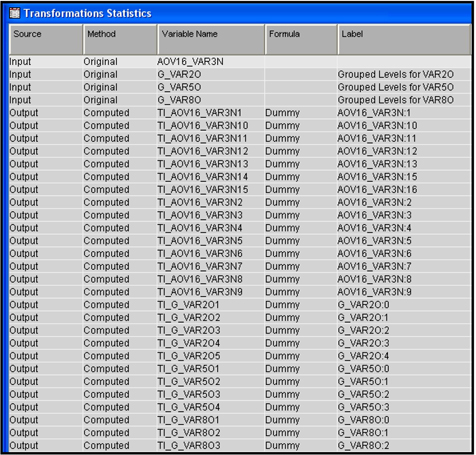
When you open the Variables window of the Variable Selection node, you can see the variables passed to it by the Transform Variables node. A partial listing of these variables is shown in Display 3.36.

Display 3.36

You can see that a log transformation of the credscore variable and a square root transformation of VAR3N made them closest to the normal distribution. No transformation could be found for VAR1N; hence, it is passed to the next node as is. If a transformation is made for a variable, then by default only the transformed variable is passed to the next node, not the original variable. If you set the Hide property to No and the Reject property to No, then both the original and transformed variables are passed to the next node that has the role set to Input.

Some of the dummy variables created for the class variable levels are also shown in Display 3.36. For example, VAR2O has eight categories. They are 0, 1, 2, 3, 4, 5, 6, and 8. Eight dummy variables (binary variables) are created (TI_VAR2O1 through TI_VAR2O8). The variable VAR2O has some missing values but no separate category is created for it. Therefore, no dummy variable is created for the missing values. The dummy variable TI_VAR2O1 takes the value of 1 if VAR2O is 0, and 0 otherwise. TI_VAR2O2 takes the value of 1 if VAR2O is 1 and 0 otherwise. TI_VAR2O3 takes the value of 1 if VAR2O is 2 and 0 otherwise, etc.

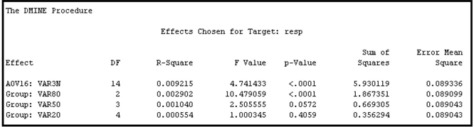
The variables selected by the Variable Selection node are shown in Output 3.16. Note that only three variables were selected, including two group variables created by the transformation. The Variable Selection node created the variable AOV16_SQRT_VAR3N because I set the Use AOV16 Variables property of the Variable Selection node to Yes.

Output 3.16

3.5.3 Transformation after Variable Selection

If you have a very large number of variables in your data set, you may want to first eliminate those that have extremely low linear correlation with the target. To achieve this, I set the values of the Minimum R-Square and Stop R-Square properties of the Variable Selection node to 0.005 and 0.0005, respectively.

The lower segment of Display 3.33 shows the process flow for transforming variables after variable selection. The Transform Variables (2) node follows the Variable Selection (2) node and precedes the Regression node.

After running the Variable Selection (2) node, open the Results window. In the Output sub-window, you can see the variables selected in Step 1 and Step 2. The variables selected in Step 1 of the variable selection are shown in Output 3.17

Output 3.17

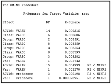
Output 3.18 shows the variables selected in Step 2.

Output 3.18

Display 3.37 shows the variables passed by the Variable Selection (2) node and the transformations done by the Transform Variables (2) node.

Display 3.37

Display 3.37 shows that the Variable Selection node created both the AOV16 variables and grouped class variables (indicated by the prefix G_), while the Transform Variables node created the dummy variables (indicated by the prefix TI) for each level of these AOV16 and grouped class variables.

Display 3.38 shows the variables passed to the Regression node.

Display 3.38

Because I set the Hide and Reject properties of the Transform Variables node to Yes, the original values of the transformed variables are not passed to the next node.

3.5.4 Passing More Than One Type of Transformation for Each Interval Input to the Next Node

3.5.4.1 Passing Two Types of Transformations Using the Merge Node

You can pass two types of transformations for each interval input to the Variable Selection or Regression node by applying two instances of the Transform Variables node. In this example, I pass Maximum Normal and Optimal Binning transformations for each interval input. In the first instance (represented by Transform Variables in Display 3.39) of the Transform Variables node, I transform all the interval inputs using the Maximum Normal transformation by setting the Interval Inputs property to Maximum Normal. In the second instance (Transform Variables (2) in Display 3.39), I transform all interval inputs using the Optimal Binning transformation by setting the Interval Inputs property to Optimal Binning.

I also set the Node ID property for each instance of the Transform Variable node. The Node ID for the first instance is Trans, and the Node ID for the second instance is Trans2.

I use the Merge node to merge the data sets created by the Transform Variables nodes so that I can pass both types of transformation to the Regression node for final selection of the variables considering both types of transformation.

Display 3.39

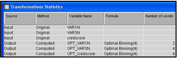
Display 3.40 shows the transformations done by the Transform Variables node in the upper segment of Display 3.39.

Display 3.40

Display 3.41 shows the transformations done by the Transform Variables node in the lower segment of Display 3.39.

Display 3.41

Display 3.42 shows the property settings of the Merge node used to combine the data sets created by the Transform Variables nodes Trans and Trans2.

Display 3.42

The Merging property is set to One-to-One because there is a one-to-one correspondence between the records of the data sets merged. Note that the Node ID property of the first instance of the Transform Variables node is Trans, and that of the second instance is Trans2.

The Variables window of the Regression node is shown in Display 3.43.

Display 3.43

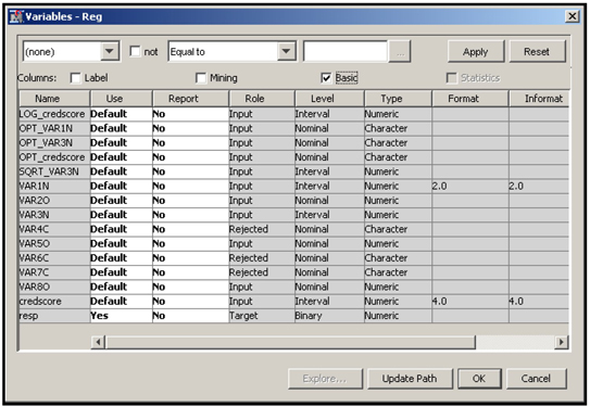
The transformations done by both the Transform Variables nodes are now available to the Regression node. In Display 3.43 you can see that the variable credscore has two types of transformation. The first one is LOG_credscore, which is created by transforming the variable credscore using the Maximum Normal method by the Transform Variables node Trans. The second transformation is OPT_credscore, created by the second instance of the Transform Variables node Trans2. In addition, the original interval variable credscore is also passed to the Regression node with its role assigned to Input since I set the Hide and Reject properties to No in both Trans and Trans2.

We can also see that the variable VAR1N has only one kind of transformation, and that it is an Optimal Binning transformation. The Maximum Normal method did not produce any transformation of VAR1N because the original variable is closer to normal than any power transformation of the original.

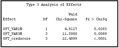
Output 3.19 shows the variables selected by the Regression node. Variable selection by the Regression node is covered in Chapter 6.

Output 3.19

Note that VAR80 is a nominal variable. The Class Inputs property for this case was set to None, so the variable was not transformed.

3.5.4.2 Multiple Transformations using the Multiple Method Property

You can send more than one type of transformation for each interval input to the Variable Selection node or the Regression node by setting the Interval Inputs property to Multiple. I set the Interval Inputs property to Multiple, the Class Inputs property to Dummy Indicators, the Hide property to No, and the Reject property to No in the Transform Variables node shown in Display 3.44.

Display 3.44

If you click located on the right of Variables property of the Regression node, you can see a list of the transformed and original variables passed to the Regression node. The inputs selected by the Stepwise Selection method of the Regression node are shown in Output 3.20.

Output 3.20

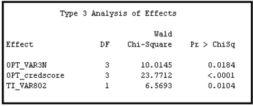
Note that TI_VAR802 shown in Output 3.20 is a dummy variable created from the variable VAR80.

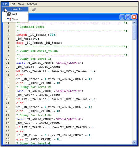
3.5.5 Saving and Exporting the Code Generated by the Transform Variables Node

You can save and export the SAS code generated by the Transform Variables node. Simply open the Results window and select View → Scoring → SAS Code from the menu bar.

To save the SAS code, select File → Save As, and then select a name for the saved file. A partial listing of the SAS code saved in my example is shown in Display 3.45.

Display 3.45

3.6 Summary

• This chapter showed how the Variable Selection node selects categorical and continuous variables to be used as inputs in the modeling process when the target is binary or continuous.

• Two criteria are available for variable selection when the target is binary: R-Square and Chi-Square.

• The R-Square criterion can be used with binary as well as continuous targets, but the Chi-Square criterion can be used only with binary targets.

• The Variable Selection node transforms inputs into binned variables, called AOV16 variables, which are useful in capturing non-linear relationships between inputs and targets.

• The Variable Selection node also simplifies categorical variables by collapsing the categories.

• The Variable Clustering node can be used for variable selection by grouping the variables that look similar in the data set, and selecting a representative variable from each group. It can also be used to combine variables that look similar.

• The Decision Tree node can also be used for variable selection. However, if you have a large number of inputs, you should make a preliminary selection by using the Variable Selection node, and then use the Decision Tree node for further selection.

• The Transform Variables node offers a wide range of choices for transformations, including multiple transformations of an input, and the option of creating dummy variables for the categories of categorical variables.

• If there are a large number of inputs, you can use the Variable Selection node to first make a preliminary variable selection, and then do transformations of the selected variables. If the number of inputs is relatively small, then you can transform all of the inputs prior to variable selection.

• The code generated by the Variable Selection node and the Transform Variables node can be saved and exported.

3.7 Appendix to Chapter 3

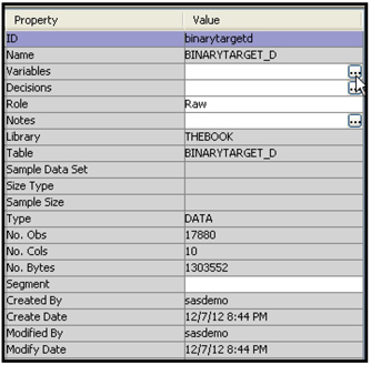
3.7.1 Changing the Measurement Scale of a Variable in a Data Source

A data source is created with the SAS table BINARYTARGET_D. To create the data source, I selected Advanced for the Metadata Advisor Option (see Displays 2.10 and 2.11). SAS Enterprise Miner marks the interval variables with less than 20 distinct levels as Nominal, unless the Class Levels Count Threshold property is set to a value other than 20 (See Display 2.11).

In the example data set BINARYTARGET_D, the variable VAR3N is a numeric variable, and it has 18 unique values. Hence, it is marked as Nominal. To change the measurement scale of this variable to interval, complete the following steps.

Under Data Sources in the Project panel, click the table name BINARYTARGET_D. Then click located in the Value column of the Variables property, as shown in Display 3.46.

Display 3.46

The Variables window appears, as shown in Display 3.47.

Display 3.47

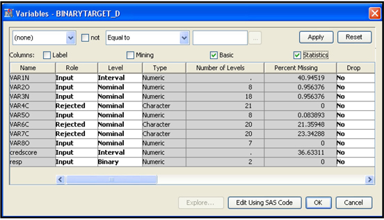
For variable VAR3N, click in the Level cell and select Interval, and then click OK. The measurement scale of the input VAR3N is changed from Nominal to Interval.

For a full discussion of the Metadata Advisor Options when creating a data source, see Section 2.5.

3.7.2 SAS Code for Comparing Grouped Categorical Variables with the Ungrouped Variables

CVAR03 has 11 categories, including the “missing” or unlabeled category, as shown in Output 3.4.

The categories of CVAR03 are grouped to create the variable G_CVAR03 with only five categories. You can compare the frequency distribution of the original variable with the grouped variables and see the mapping of the categories of CVAR03 into G_CVAR03 using the SAS code shown in Display 3.48.

Display 3.48

Exercises

1. Create a data source using the SAS data set Attrdata3_New.

2. Select Basic for the Metadata Advisor Option.

3. Set the model role of the variable Event to Target, and set its measurement level to Binary.

4. Open the Prior Probabilities tab of the Decision Configuration step and enter the following prior probabilities in the Adjusted Prior column: 0.024 for level 1 and 0.976 for level 0.

5. Create the following process flow diagram.

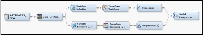
In the Data Partition node, allocate 50% of the observations for Training and 50% for Validation.

In the Variable Selection node located in the upper segment of the process flow diagram, set the Target Model property to R-Square and the Use AOV16 Variables property to No.

In the Transform Variables node located in the upper segment of the process flow diagram, set the Interval Inputs property to Optimal Binning, and set the Class Inputs property to Dummy Indicators.

In the Variable Selection node located in the lower segment of the process flow diagram, set the Target Model property to R-Square and the Use AOV16 Variables property to Yes.

In the Transform Variables node located in the lower segment of the process flow diagram, set the Interval Inputs property to Best, and set the Class Inputs property to Dummy Indicators.

In both the Regression nodes, set the Selection Model property to Stepwise and the Selection Criterion to Validation Error.

Run all the nodes in sequence. Then open the Results window of the Model Comparison node, examine the Cumulative % Captured Response plot, and get a preliminary assessment of which model is better—the one generated by the sequence of nodes in the upper segment of the process flow diagram or the one generated by the lower segment?

Using the following table, calculate % Response, Cumulative % Response, %Captured Response, Cumulative Captured Response, Lift and Cumulative Lift by Bin/Percentile.

Note

1. The SAS manuals often use the term “Class” instead of “Categorical.” I use these two terms synonymously.

..................Content has been hidden....................

You can't read the all page of ebook, please click here login for view all page.

Table of Contents for Chapter 3: Variable Selection and Transformation of Variables

Create new playlist

Sign In

Sign Up

Chapter 3: Variable Selection and Transformation of Variables

3.1 Introduction