
1 On the Principles of Quantum Control Theory
Re-Bing Wu, Jing Zhang and Tzyh-Jong Tarn
CONTENTS
1.2 Mechanism of Quantum Control
1.3 Modeling and Analysis of Quantum Control Systems
1.4 Control Design Methodologies
1.4.1 Open-Loop Control of Quantum Systems
1.4.2 Closed-Loop Control of Quantum Systems
1.1 Introduction
In his 1959 famous lecture "Plenty of Room at the Bottom" [19], Richard Feynman considered the possibility of manipulating and controlling things at microscopic scales in the near future. Now his prediction has become reality with system assembly at the nanoscale level. When such systems are at a sufficiently low temperature, quantum effects will appear. From a cybernetical point of view, quantum control is a very useful theory for solving relevant problems in measurement, information transmittal, and state engineering.
What makes quantum control interesting are the nonclassical features of quantum mechanics. Unlike the classical world, the wave–particle duality sets no explicit boundary between particles and waves. An electromagnetic field can be quantized into particle-like photons, and wavelike properties such as diffraction can be observed with an atom or an electron. This makes it possible to manipulate waves like particles or vice versa. In other words, the essence of quantum control is to manipulate the coherence properties.
Early works on quantum control were motivated by control problems in plasma and laser devices, nuclear accelerators, and nuclear power plants [9–11]. In the 1980s, a serial study was casted to the modeling [46], controllability [24], invertibility [31], and quantum nondemolition filter problems [13]. Meanwhile, in Europe Belavkin started investigating filtering problems in quantum state estimation and feedback control applications [2-4]. Later, photonic control of chemical processes using lasers inspired a large number of quantum control studies that are still active today [1,36,37,43,49]. During this period, optimal control theory (OCT) was introduced to pulse shape design [33,45] based on known quantum Hamiltonians for the controlled molecules. In 1992, model-independent learning optimization algorithms [26] for real laboratory controls were proposed, which has led to over 150 successful experimental applications [7].
In the late 1990s, another tide of quantum control applications was developed by quantum information sciences. Since elementary quantum bits can be physically constructed by natural and artificial atoms (e.g., trapped ions, quantum dots, and superconducting circuits [8,22]), solving typical control problems, for example, state initialization, gate operation, error correction, and networking of quantum computers, is key to hardware implementation of quantum information processors.
The field of quantum control is still growing rapidly. Several monographs have been published on quantum control by authors from chemistry, quantum optics, and control theory [16,37,43,50], and on the state-of-art of quantum control from various review articles [7,17,47]. This chapter sketches fundamental concepts and problems in quantum control theory. In Section 1.2, physical mechanisms behind quantum control theory are discussed. Modeling and analysis problems are introduced in Section 1.3 In Section 1.4, open-loop and feedback control methods are briefly summarized. Finally, perspectives are presented.
1.2 Mechanism of Quantum Control
A nanoscale system can be modeled as either classical or quantum, although the former is nothing but an approximation of the latter under proper physical conditions. Mathematically, the quantum description is quantized from a classical model by replacing physical observables with operators that satisfy certain commutation relationships. In particular, to characterize the dynamics of quantum systems, it is essential to know the Hamiltonian that involves a potential energy function. As shown in Figure 1.1, the value of potential energy of a classical system can be an arbitrary real number. However, in quantum systems, only eigenvalues of the operator corresponding to the Hamiltonian can be recognized by a classical observer; they are called the energy levels. When the potential is a well, the energy levels are usually discrete, and the number of levels can be infinite when the well is infinitely deep (Figures 1.1b,c). The discretization of energy values is where we get the terminology "quantum," but it should be clarified that quantum energy levels are not always discrete, because a continuous spectrum (see Figure 1.1a) can exist when the energy is beyond the top of the potential.
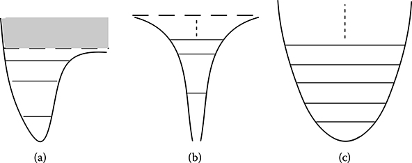
FIGURE 1.1
Spectrum with four different potentials: (a) potential well with finite depth, where both discrete (lower horizontal lines) and continuous levels (upper shaded area) exist; (b) an infinitely deep potential that is lower bounded; (c) an infinitely deep potential that is upper bounded.
These classically discernable levels form an orthogonal basis of the Hilbert space on which the quantum observables operate. Any physically admissible states can be expressed as a linear combination (with complex coefficients) of these basis vectors. In the so-called Schrödinger picture, the coefficients represent the probability amplitude of the corresponding states. For example, suppose a quantum system has only two energy levels, e1 and e2, then any physical allowable state (after normalization) can be expressed as
where |c1,2|2 represents the probability of the system staying at the state e1,2. The phase difference between complex numbers c1 and c2 manifests the wavelike coherence feature of the quantum system.
Any physically measurable quantity can be represented by an operator Ô defined on the same Hilbert space, whose eigenvalues correspond to its recognizable values by a classical observer. Its expectation value under a quantum state Ψ in the Hilbert space is calculated by the quadratic form (Ô) = Ψ†ÔΨ. These notations enable us to describe the famous Heisenberg uncertainty principle,
which reveals that two arbitrary noncommutative observables cannot be simultaneously precisely measured.
Control actions in quantum systems are based on the physical interaction between matter (e.g., atoms, ions, nuclear spins or quantum dots) and field (e.g., x-ray, light, or radio-frequency waves). Accordingly, the object to be controlled can be either a field or some matter. The control of matter is usually done using manipulable electromagnetic fields (see Figure 1.2a), while the control of field is done using a properly designed structure of the waveguide (e.g., photonic crystals, Figure 1.2b). It is also possible to use one field to control another field, but this has to be done with some linear or nonlinear medium because there is no direct interaction between electromagnetic fields.
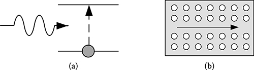
FIGURE 1.2
Schematics for quantum control scenarios based on field-matter interactions: (a) a two-level atom is controlled by a coherent field, and (b) a quantum field going through a bulk optimal medium is controlled by designed structures.
For example, shaped coherent (laser) fields are widely used to manipulate quantum molecular dynamics. When the photon number contained in the field is large (~105/cm3 in each mode), the field amplitude can be approximated with high precision by its average value, which can be taken as a classical electromagnetic field. Moreover, when the size of the matter being radiated is far smaller than the wavelength of the light, the interaction with the field is only dependent on the position of the center of mass. Under properly chosen gauge, the interaction Hamiltonian can be written as
where D is the dipole operator of the quantum system and the control field parameter E(·) is taken to be classical. When the size of the matter is comparable with the wavelength, a coupled Maxwell equation representing the evolution of the field will be required.
To simplify the analysis and design, it is always desirable to separate from the field-matter interacting system a minimal subsystem whose quantum effects cannot be ignored, and treat the rest as a classical system. Generally, a system has to be described by quantum mechanics if the fluctuation of the concerned observable is comparable with the gap between the eigenvalues of the observable. The following criteria are frequently used:
The control precision is comparable with the Heisenberg uncertainty.
An atom (natural or artificial) is taken as quantum when the environment temperature T is so low that the thermal fluctuation kT, where k is the Boltzmann constant, is smaller than the quantum energy gap δE.
An optical field is taken as quantum if it does not contain sufficiently many photons.
Following these rules, in the next section we introduce the general model of quantum control systems and an analysis of its controllability properties.
1.3 Modeling and Analysis of Quantum Control Systems
The evolution of the quantum state Ψ(t) is governed by the following Schrödinger equation:
where is the operator quantized from the classical Hamiltonian defined on the Hilbert space.
Without any classical approximation, the evolution of the joint state Ψtot(t) of the controller and the system can be written as
where the control is a time-dependent operator defined on the controller's Hilbert space. When the control can be treated as a classical variable, we can obtain the following bilinear quantum control system:
where Ψ(t) is the quantum state of the system to be controlled. The operator H0 is the internal Hamiltonian, and Hk is the control Hamiltonian via time-dependent control parameters uk(t). Here, the quantum system to be controlled can be either matter or field.
In quantum information sciences, the implementation of a quantum algorithm requires a directed evolution represented by the unitary operator U(t) such that Ψ(t) = U(t)Ψ(0) for any initial state Ψ(0). The control of U(t) is described as follows:
where U(0) is always an identity operator (i.e., nothing is changed at the beginning of control).
Controllability is referred to as the ability to steer quantum systems between arbitrary states (or evolution operators) by varying the control in Equations 1.3, 1.4, or 1.5. From a practical point of view, it appears that controllability is not so important because not all state transitions are desired. However, a recent study [53] revealed that the loss of controllability may increase the complexity of finding optimal controls (i.e., search efforts)—the more the system is controllable, the easier is the search to reach a global optimal solution. Thus, it is warranted to delve further into the fundamental study of controllability.
First described in the early 1980s, the controllability criterion was proposed in terms of rank conditions of the Lie algebra generated by the system's free and control. Hamiltonians. This was later extended to time-dependent systems [29] and systems with an infinite-dimensional controllability Lie algebra generated by internal and control Hamiltonians in Equation 1.4 [54]. Recently, a geometric analysis [6] showed that a two-level system interacting with a single optical mode is controllable over any finite-dimensional subspace without rotating-wave approximation, which is crucial for understanding the dynamics of strongly interacting quantum systems.
The controllability of infinite-dimensional systems, in particular those with unbounded or continuous spectrum, is extremely difficult because the set of states accessible from a fixed initial state is at the most dense in the Hilbert space. Therefore, the controllability will always have to be studied in a proper domain on which the functional analysis makes sense [24,54]. The results on a finite-dimensional case are much richer. For example, for molecular systems that can be approximated as finite dimensional, there are many studies on controllability with respect to the dipole structure [42] and degeneracies of the levels. With respect to the fully quantum model (1.3), an interesting result [38] shows that the state of a two-level system can be completely controlled by tuning the initial state of a coupled two-level system. Controllability of general systems can be enhanced by enriching the entanglement with the control source (or probe).
The previously mentioned studies assume that the quantum system to be controlled can be well isolated from the environment and can be precisely addressed by the control source. A typical example is the IVR (intramolecular vibrational resonance) that hindered the control of molecular reactions for quite a long time. Such uncontrollable environment interaction should be integrated into the model as a noise or a dissipation term [50], which may drive the system dynamics to its classical limit. Except when the control process can be completed within the decoherence time (e. g., in ultrafast control experiments), active controls should be posed against the decoherence effect. This is a fundamentally important control problem in quantum control theory [14,48,55].
1.4 Control Design Methodologies
The terminology "quantum control" is used rather loosely in the literature, as any attempt to choose a parameter can be called quantum control no matter what method is used. If the model can be precisely constructed and no significant disturbances exist, the open-loop control will be sufficient without having to measure the system output [7]. Otherwise, feedback control needs to be introduced for correcting the errors according to the measured result of the evolving state [17]. According to whether the controller and the plant are quantum or classical, one can classify the structure of the control system into the following four types:
Open-loop control (Figure 1.3a): The controller is treated as a classical system that has unidirectional causal action on the system.
Direct coherent feedback control (Figure 1.3b): The controller is treated as a quantum system with bidirectional causal relation with the system.
Measurement-based feedback control (Figure 1.3c): The controller is treated as a classical system that adjusts itself according to the classical information acquired from the measurement result of the system.
Field-mediated coherent feedback control (Figure 1.3d): The controller is treated as a quantum system with control loop closed by unidirectional field mediation.
1.4.1 Open-Loop Control of Quantum Systems
Open-loop control is the simplest and most broadly used control structure in the literature. Some of the open-loop control strategies were from physical intuition (e.g., dynamical decoupling method learned from the spin-echo phenomena in NMR systems [5,12]), and some were designed by more universal quantum optimal control theory and algorithms. In the following, we introduce the basic idea of quantum optimal control theory in the literature.
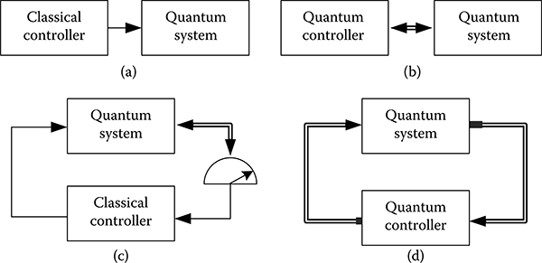
FIGURE 1.3
Types of quantum control: (a) open-loop control; (b) direct coherent feedback control; (c) measurement-based feedback control; and (d) field-mediated coherent feedback control.
Every target of control can be characterized by one or multiple costs as functional(s) of the control function, say J[u(£)]. For example, the length of a chemical bond to be broken in chemical reactions can be taken as a cost to be maximized. Other cost functionals are, for example, the state transition probability [5], gate fidelity [32], coherence degree [55], fluence minimization [15], and the time consumed for control [27]. According to the Schrödinger equation (taken as a restriction on the control and state), one can derive the necessary condition for some u(t) to minimize the cost functional if the control functions are not restricted. Otherwise, the generalized maximum principle [16] must be introduced to deal with the restrictions (e.g., limited field strength or bandwidth).
The optimal control is obtained by resolving the equations set by the necessary condition. When such equations (usually appearing in the form of nonlinear differential equations) are not analytically solvable, iterative algorithms can be designed to search the solution from an initial guess. From the control model Equation 1.4, it is possible to calculate the gradient of the cost with respect to the control function, following which a gradient-type algorithm [28,39,40] can be designed to steer the search of control solutions toward an optimal one. Iterative-type algorithms generally converge quickly, but can easily diverge if the initial guess was improperly chosen. By contrast, gradient-type algorithms are more stable as long as the step-size is sufficiently small, but the drawback is their convergence is very slow especially near the optimal solutions.
Quantum optimal control theory has been proven to be effective for finite-level or simple few-body systems [7]. However, the system Hamiltonians have to be precisely known, which is almost impossible in the laboratory. Even when the Hamiltonian is available, heavy computation will be not realistic on the numerical integration of the time-dependent Schrödinger equation in each iteration. To avoid this difficulty, evolutionary-type algorithms [26,44] were proposed (see Figure 1.4), where only the measurement output is needed for iterating the control function. This actually leaves the most difficult part of computation done by nature. Therefore, although the convergence may be much slower, learning algorithms are advantageous in the laboratory because not every detail of the real system must be known.

FIGURE 1.4
Schematic diagram of iterative learning control. The chemical reaction is controlled by a shaped laser pulse that is iteratively adjusted according to the measurement result. In each iteration, the control is performed on a fresh sample prepared at the same initial state.
In quantum optimal control theory, all algorithms may suffer from the possible existence of false traps, that is, the search may converge to an undesired locally optimal solution that is not globally optimal. When the resource for optimization is not sufficient, the trapping behavior will become more severe. However, quick convergence was observed toward global optimal solutions in most reported simulations, and the reported experimental yields were remarkably improved as well [34]. This implies that traps are rare in practical control of quantum systems. Recently, this conjecture was supported via geometric analyses on the so-called quantum control landscape [34]. It was proven that if the system is controllable, then upon some mild assumptions there exist no obstacles on the landscape for maximization of observable expectation value [52], gate fidelity [35] in both closed and open systems [51]. Quantum control landscape theory has grown into a new research field, from which the details of the geometric landscape structure will provide greater understanding of quantum control and optimization so that more efficient algorithms can be developed.
1.4.2 Closed-Loop Control of Quantum Systems
In contrast to classical control theory, the body of literature on open-loop control is much larger than that of feedback control. This is not because feedback control is disadvantageous, but because the measurement required for feedback is much more difficult than what can be done with the control. The trade-off between inevitable backaction and the obtained information needs to be well understood. Nevertheless, quantum feedback control has already become a worldwide focus, as indicated by the 2012 Nobel Prize in physics awarded to Haroche and Wineland [23,41].
Measurement-based feedback control strategies can be further divided into two classes. The first is Markovian quantum feedback developed by H. M. Wiseman and G. J. Milburn [50], where quantum continuous weak measurement is adopted for feedback. With an idea learned from the quantum trajectory theory developed in quantum optics, the backaction of the measurement on the system is modeled as classical noise (either discontinuous jump noise or continuous Wiener white noise) that disturbs the system dynamics. The other approach is the Bayesian feedback control, initially proposed by A. C. Doherty [18], where the control strategy is determined based on the estimated state from the measurement output. The estimator is also called a "quantum filter" [2]. In principle, Bayesian feedback may outperform the Markovian feedback because more information extracted from the measurement history can be used to determine the control.
In addition to the backaction, the measurement-based feedback approaches are mainly limited by the time scale of quantum dynamics, which is often too fast to be followed by a classical controller. Regarding these difficulties, coherent feedback strategies have received much attention in recent years. As proposed by S. Lloyd [30], the simplest way to introduce coherent feedback is to couple directly the controlled quantum system to the quantum controller (Figure 1.3b). An alternative approach that is closer to measurement-based feedback control is field-mediated coherent feedback, where the quantum signal is carried by an intermediate field from the system to the controller (Figure 1.3d). This approach [21,25] was based on the quantum description of input-output theory developed by Gardiner et al. [20] in the 1980s. Compared with measurement-based feedback, the coherent feedback loop is more easily realized in experiments, thereby making it more suitable for scalable control circuits in future applications.
1.5 Perspectives
Quantum control is a developing field that is open to studies in various areas. Limited by fundamental experimental technologies for manipulating and observing quantum phenomena, experimental application of quantum control is still in its infancy except for the case of learning control. The fusion of control theory and quantum physics calls for collaborations between physicists and engineers. In the past decade, the gap between physicists and engineers has been greatly reduced, along with the rapidly developing experimental technologies and emerging common interests. There will be, undoubtedly, tremendous research opportunities for engineers in nanotechnology in the next decades.
Acknowledgments
The authors acknowledge support from NSFC (No. 60904034, 61134008, 61174084) and the Tsinghua National Laboratory for Information Science and Technology (TNList) Cross-Discipline Foundation.
References
1. Bandrauk, A., Delfour, M., and Bris, C. L. (eds.). Quantum control: Mathematical and numerical challenges, CRM Proceedings and Lecture Notes, vol. 33. American Mathematical Society, Providence (2003).
2. Belavkin, V. Optimal quantum filtration of Markovian signals. Problems of Information Transmission 7(5), 1-14 (1978).
3. Belavkin, V. and Grishanin, B. Optimum estimation in quantum channels by the generalized Heisenberg inequality method. Problems of Information Transmission 9(3), 209-215 (1972).
4. Belavkin, V and Grishanin, B Optimum measurement of quantum variables. Problems of Information Transmission 8(3), 259-265 (1972).
5. Bergmann, K., Theuer, H., and Shore, B. W. Coherent population transfer among quantum states of atoms and molecules. Reviews of Modern Physics 70, 1003-1025 (1998)
6. Bloch, A., Brockett, R., and Rangan, C. Finite controllability of infinite-dimensional quantum systems. IEEE Transactions on Automated Control 55(8), 1797-1805 (2010)
7. Brif, C., Chakrabarti, R., and Rabitz, H. Control of quantum phenomena: Past, present, and future. New Journal of Physics 12, 075,008 (2010).
8. Buluta, I., Ashhab, S., and Nori, F. Natural and artificial atoms for quantum computation. Reports on Progress in Physics 74(10), 104,401 (2011). DOI 10.1088/0034-4885/74/10/104401.
9. Butkovskii, A. and Pustyl'nikova, E. Controlling the coherent states of a quantum oscillator. Automation and Remote Control 43, 1393-1398 (1982).
10. Butkovskii, A. and Pustyl'nikova, E. Control of coherent states of quantum systems with a quadratic Hamiltonian. Automation and Remote Control 45, 1000-1008 (1984).
11. Butkovskii, A. and Samoilenko, Y. Control of quantum-mechanical processes and systems, Mathematics and Its Applications, vol. 56. Kluwer Academic Publishers, Boston (1990).
12. Chelkowski, S. and Bandrauk, A.D. Raman chirped adiabatic passage: A new method for selective excitation of high vibrational states. Journal of Raman Spectroscopy 28(6), 459-466 (1997).
13. Clark, J., Ong, C., Tarn, T.J., and Huang, G.M. Quantum nondemolition filters. Mathematical Systems Theory 18, 33-55 (1985).
14. Clausen, J., Bensky, G., and Kurizki, G. Bath-optimized minimal-energy protection of quantum operations from decoherence. Physical Review Letters 104(4) (2010). DOI 10.1103/PhysRevLett.104.040401.
15. D'Alessandro, D. Optimal control of two level quantum systems. IEEE Transactions on Automatic Control 46, 866-876 (2001).
16. D'Alessandro, D. Introduction to Quantum Control and Dynamics. Chapman & Hall/CRC, Boca Raton (2008).
17. Daoyi, D. and Petersen, I. Quantum control theory and applications: A survey. IET Control Theory and Applications 4(12), 2651-2671 (2010).
18. Doherty, A.C., Habib, S., Jacobs, K., Mabuchi, H., and Tan, S.M. Quantum feedback control and classical control theory. Physical Review A 62, 012,105 (2000).
19. Feynman, R. There's plenty of room at the bottom. Annual Meeting of the American Physical Society, California Institute of Technology, Pasadena, CA (December 29, 1959).
20. Gardiner, C.W. and Collett, M.J. Input and output in damped quantum systems: Quantum stochastic differential equations and the master equation. Physical Review A 31, 3761-3774 (1985).
21. Gough, J. and James, M. The series product and its application to quantum feedforward and feedback networks. IEEE Transactions on Automatic Control 54(11), 2530-2544 (2009).
22. Grigorenko, I. and Rabitz, H. Optimal control of the local electromagnetic response of nanostructured materials: Optimal detectors and quantum disguises. Applied Physics Letters 94(25), 253107 (2009).
23. Hinds, E. and Blatt, R. Nobel 2012 physics: Manipulating individual quantum systems. Nature 492(7427), 55 (2012).
24. Huang, G.M., Tarn, T.J., and Clark, J.W. On the controllability of quantum-mechanical systems. Journal of Mathematical Physics 24, 2608-2618 (1983).
25. James, M., Nurdin, H., and Petersen, I. Control of linear quantum stochastic systems. IEEE Transactions on Automatic Control 53(8), 1787-1803 (2008).
26. Judson, R. and Rabitz, H. Teaching lasers to control molecules. Physical Review Letters 68, 1500 (1992).
27. Khaneja, N., Brockett, R., and Glaser, S. Time optimal control in spin systems. Physical Review A 63(3), 032,308 (2001).
28. Khaneja, N., Reiss, T., Kehlet, C., Schulte-Herbrüggen, T., and Glaser, S.J. Optimal control of coupled spin dynamics: Design of NMR pulse sequences by gradient ascent algorithms. Journal of Magnetic Resonance 172, 296-305 (2005).
29. Lan, C., Tarn, T.J., Chi, Q.S., and Clark, J.W. Analytic controllability of time-dependent quantum control systems. Journal of Mathematical Physics 46(5), 052102 (2005).
30. Lloyd, S. Coherent quantum feedback. Physical Review A 62, 022,108 (2000).
31. Ong, C., Huang, G., Tarn, T., and Clark, J. Invertibility of quantum-mechanical control systems. Mathematical Systems Theory 17(4), 335-350 (1984).
32. Palao, J.P. and Kosloff, R. Quantum computing by an optimal control algorithm for unitary transformations Physical. Review Letters 89, 188,301 (2002).
33. Peirce, A., Dahleh, M., and Rabitz, H. Optimal control of quantum-mechanical systems: Existence, numerical approximation, and applications. Physical Review A 37, 4950-4964 (1988).
34. Rabitz, H., Hsieh, M., and Rosenthal, C. Quantum optimally controlled transition landscapes. Science 303(5666), 1998-2001 (2004).
35. Rabitz, H., Hsieh, M., and Rosenthal, C. The landscape for optimal control of quantum-mechanical unitary transformations. Physical Review A 72, 52,337 (2005).
36. Rabitz, H., de Vivie-Riedle, R., Motzkus, M., and Kompa, K. Whither the future of controlling quantum pheonomena? Science 288, 824-828 (2000).
37. Rice, S. and Zhao, M. Optical Control of Molecular Dynamics. John Wiley & Sons, New York (2000).
38. Romano, R. and D'Alessandro, D. Environment-mediated control of a quantum system. Physical Review Letters 97, 080,402 (2006).
39. Rothman, A., Ho, T.S., and Rabitz, H. Observable-preserving control of quantum dynamics over a family of related systems. Physical Review A 72(2), 023416 (2005).
40. Rothman, A., Ho, T.S., and Rabitz, H. Quantum observable homotopy tracking control. Journal of Chemical Physics 123(13), 134104 (2005).
41. Sayrin, C., Dotsenko, I., Zhou, X., Peaudecerf, B., Rybarczyk, T., Gleyzes, S., Rouchon, P., Mirrahimi, M., Amini, H., Brune, M., Raimond, J.M., and Haroche, S. Real-time quantum feedback prepares and stabilizes photon number states. Nature 477(7362), 73-77 (2011).
42. Schirmer, S.G., Fu, H., and Solomon, A. I. Complete controllability of quantum systems. Physical Review A 63(6), 063,410 (2001).
43. Shapiro, M. and Brumer, P. Principles of the Quantum Control of Molecular Processes. Wiley-Interscience, Hoboken (2003).
44. Shir, O., Beltrani, V., Bäck, Th., Rabitz, H., and Vrakking, M. On the diversity of multiple optimal controls for quantum systems. Journal of Physics B 41(7), 074,021 (2008).
45. Tannor, D., Kosloff, R., and Rice, S. Coherent pulse sequence induced control of selectivity of reactions: Exact quantum mechanical calculations. Journal of Chemical Physics 85(10), 5805-5820 (1986).
46. Tarn, T.J., Huang, G.M., and Clark, J. Modelling of quantum mechanical control systems. Mathematical Modelling 1, 109-121 (1980).
47. Vandersypen, L. and Chuang, I. NMR techniques for quantum control and computation. Reviews of Modern Physics 76(4), 1037-1069 (2004).
48. Viola, L. and Lloyd, S. Dynamical suppression of decoherence in two-state quantum systems. Physical Review A 58(4), 2733-2744 (1998) DOI 10 1103/PhysRevA 58 2733.
49. Warren, W., Rabitz, H., and Dahleh, M. Coherent control of quantum dynamics: The dream is alive. Science 259, 1581-1588 (1993).
50. Wiseman, H. Quantum Measurement and Control. Cambridge University Press, Cambridge (2010).
51. Wu, R., Pechen, A., Rabitz, H., Hsieh, M., and Tsou, B. Control landscapes for observable preparation with open quantum systems. Journal of Mathematical Physics 49, 022,108 (2008).
52. Wu, R., Rabitz, H., and Hsieh, M. Characterization of the critical submanifolds in quantum ensemble control landscapes. Journal of Physics A 41, 015,006 (2008).
53. Wu, R.B., Hsieh, M.A., and Rabitz, H. Role of controllability in optimizing quantum dynamics. Physical Review A 83, 062,306 (2011).
54. Wu, R. B., Tarn, T.J., and Li, C. W. Smooth controllability of infinite-dimensional quantum-mechanical systems. Physical Review A 73, 012,719 (2006).
55. Zhang, J., Li, C.W., Wu, R.B., Tarn, T.J., and Liu, X.S. Maximal suppression of decoherence in Markovian quantum systems. Journal of Physics A: Mathematical and General 38(29), 6587 (2005).