9 Hybrid Control for Micro/Nano Devices and Systems

Search in book...
Toggle Font Controls
Create new playlist

Name your new playlist

Playlist description (optional)
Sign In

Email address

Password

Forgot Password?

or

Continue with Facebook

Continue with Google
Sign Up

Full Name

Email address

Confirm Email Address

Password

or

Continue with Facebook

Continue with Google

Xiaobo Li, Xinghua Jia and Mingjun Zhang

9.1 Introduction

9.2 Problem Formulation

9.3 Control Framework, Control Design, and Analysis

9.3.1 Control Framework

9.3.2 Feedforward Control Design

9.3.3 Design of Time-Driven and Data-Driven Planners

9.3.4 Planners Switching Control Mechanism

9.3.5 Robustness Analysis

9.1 Introduction

Regulation mechanisms in biological systems usually employ two basic control structures: feedback and feed- forward [1]. Hybrid feedback and feed-forward control structures are common in biological systems. Biological regulation mechanisms can also be categorized as having either data-driven control or time- driven control. Compared to the prevalence of feedback and time- driven controls, theoretical investigations and practical applications of feed- forward and data- driven controls are not new [2–9]. One work was presented in Reference 10, where the inversion- based feed- forward control design was introduced for output tracking of nonlinear systems. It is applicable to multiple- input and multiple- output (MIMO) nonminimum phase systems through calculating the noncausal inverse. For the nonminimum phase systems, a preview- based feed- forward output tracking control was proposed and used for scanning tunneling microscopy control [11]. However, these methods did not take advantage of the feedback measurement. Data- driven control has also been proposed in robotic trajectory planning, regulation of the outputs of biological systems by controlling microenvironement, etc. [8,9,11]. Motivated by the need in gene therapy, a data- driven feed- forward control mechanism that integrates the feed- forward control and data-driven control has been proposed in Reference 12. However, the method proposed is only for single- input– single- output (SISO) minimum- phase systems with continuous measurement. It may not work when the measurement is in a hybrid format, a case that prevails in biological cellular systems and multi- scale engineering systems.

Inspired by regulation mechanisms of biological systems, we propose in this chapter a hybrid time- data- driven control framework for micro-/nanoscale devices or systems with hybrid sensing signals. This is significant for developing a control theory for manipulation of cellular systems and for controlling micro-/nanoscale engineered systems. In this work, we first develop an inverse- based feed- forward control to track the reference trajectory that is generated by either a time- driven or data- driven reference generator (this is due to the nature of biological cellular systems, so that we need the hybrid combination). Depending on the real- time availability of the measurement, the control system is able to switch itself between the data-driven control and the time- driven control.

This study aims to make several original contributions in controlling micro-/nanoscale systems. First, compared to the data- driven feed- forward control proposed previously [12], this new approach can be applied to MIMO biological cellular system control. In addition, compared to the standard time- driven and data- driven approach [12], the proposed control is applicable to measurements with any hybrid format. In principle, each channel can accommodate signals in different formats, including no signal, continuous-time signal, discrete- time signal, and hybrid signal in cases where that signal is either continuous or discrete.

This work is motivated by the need to externally control biological cellular systems for bioengineering applications, where the need is fast emerging from nanomedicine and molecular and cellular engineering. However, there is no control theory available for the purpose. For cellular control, accessible measurement is not always persistent, but often exhibits a hybrid characteristic. In addition, to control biological cellular systems requiring rapid response in nanoscale, a feedback control is not guaranteed to be effective due to relatively slow measurements.

9.2 Problem Formulation

Most micro/nanoscale devices and systems can be modeled as MIMO nonlinear dynamic systems, where partial inputs can be externally manipulated and partial outputs may be measured in real time [1,13]. Here we can use the following generic MIMO nonlinear dynamical model to describe biological systems.

\begin{matrix} \dot{x} & = & f (x) + g (x) u \\ y & = & h (x) \end{matrix} (9.1)

$\begin{matrix} \dot{x} & = & f (x) + g (x) u \\ y & = & h (x) \end{matrix} (9.1)$

where x ÎRⁿ, u Î R^q and y ÎR^q are the state, the input, and the output, respectively, and f(x), g(x), and h(x) are smooth vector fields with compatible dimensions. Without loss of generality, we assume that f(0) = 0 and h(0) = 0. The control objective is to design a control input u, using the available measurement y, such that the output y tracks a reference signal y_d(t). Here, the tracking control problem means that the trajectory of y follows y_d(t) in terms of the data space. This control problem is critically needed in cellular system control [1,13]. We make two assumptions.

Assumption 1. The origin of the linearized system

\dot{x} = {\frac{d f (x)}{d x} |}_{x = 0} x = : A x

$\dot{x} = {\frac{d f (x)}{d x} |}_{x = 0} x = : A x$

is stable.

Assumption 2. The system (Equation 9.1) has a well-defined relative degree r = (r₁, r₂, …, r_q) at the origin [14].

Remark 1. Assumption 1 is straightforward, since cellular systems are stable in the health state, which was assumed as origin in almost all practices of cellular system modeling. Assumption 2 requires thatβ be nonsingular. This requirement can be relaxed by adding integrators [40].

Remark 2. Devasia et al.’s paper [10] requires the assumption that the system (9.1) has a minimum phase. However, this assumption is not required in this study. Specifically, if the system (9.1) is a nonminimum phase, the noncausal inverse can be employed to compute the internal dynamics through the integration of a backward differential equation [10].

Images

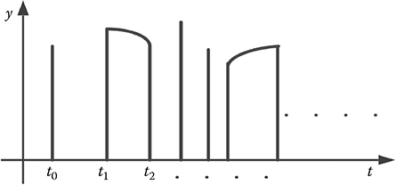
FIGURE 9.1
Illustration of the signal formats of different measurements.

Images

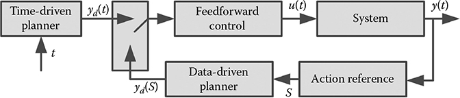
FIGURE 9.2
The proposed hybrid time– data- driven control framework.

9.3 Control Framework, Control Design, and Analysis

9.3.1 Control Framework

Figure 9.1 shows the general measurement format. It includes three possible cases: (1) no measurement, (2) continuous measurement, and (3) isolated measurement. It is common in cellular system control in which persistent measurement is not easy due to the measurement technique. In addition, for a MIMO system with multiple output channels, each channel could have its own measurement format.

The proposed hybrid time– data- driven control framework is shown in Figure 9.2. The inverse-based feed- forward control is to make the output y track the reference trajectory y_d. The reference trajectory is produced by either the time- driven planner or the data- driven planner. The two independent planners are able to be switched, depending on the real- time form of the measurement outputs. When no measurement is available, the time- driven controller will be used. When continuous- time measurement is available, the data- driven controller will be used if certain conditions can be met. Thus, when the measurement arrives in a discrete- time manner, or hybrid form, then the hybrid time– data- driven control is obtained. The data- driven planner is triggered by an event. This control approach covers the classical time- driven and data- driven controls as two special cases.

9.3.2 Feedforward Control Design

The idea is to take the inverse of the original system (9.1) as the feed- forward control [14], based on the exact linearization. Define

r = Σ_{i = 1}^{q} r_{i}

$r = Σ_{i = 1}^{q} r_{i}$

By Assumption 2, y_i(·) can be differentiated r_i times so that one u_j(t) appears explicitly [10]. Define $ξ_{k}^{i} (t) = y_{i}^{(k - 1)} (t)$ $ξ_{k}^{i} (t) = y_{i}^{(k - 1)} (t)$ and i = 1, 2, …, q, and denote

\begin{matrix} ξ (t) & = & [\begin{matrix} ξ_{1}^{1} (t) & ξ_{2}^{1} (t) & \dots & ξ_{r}^{1} (t) & ξ_{1}^{2} (t) & \dots & ξ_{r 2}^{2} (t) & \dots & ξ_{r_{q}}^{q} (t) \end{matrix}]^{T} \\ = & [\begin{matrix} y_{1} (t) & \dot{\begin{matrix} y_{1} \end{matrix}} (t) & \dots & y_{1}^{(r_{1} - 1)} (t) & y_{2} (t) & \dots & y_{2}^{(r_{2} - 1)} (t) & \dots & y_{q}^{(r_{q} - 1)} \end{matrix} (t)]^{T} \end{matrix}

$\begin{matrix} ξ (t) & = & [\begin{matrix} ξ_{1}^{1} (t) & ξ_{2}^{1} (t) & \dots & ξ_{r}^{1} (t) & ξ_{1}^{2} (t) & \dots & ξ_{r 2}^{2} (t) & \dots & ξ_{r_{q}}^{q} (t) \end{matrix}]^{T} \\ = & [\begin{matrix} y_{1} (t) & \dot{\begin{matrix} y_{1} \end{matrix}} (t) & \dots & y_{1}^{(r_{1} - 1)} (t) & y_{2} (t) & \dots & y_{2}^{(r_{2} - 1)} (t) & \dots & y_{q}^{(r_{q} - 1)} \end{matrix} (t)]^{T} \end{matrix}$

Chooseη, an n−r- dimensional function on Rⁿ, so that [ξ^T, η ^T]^T = φ(x) forms a change of coordinates withφ(0) = 0. With these new coordinates, the system dynamics (9.1) leads to

{\dot{ξ}}_{r_{i}}^{i} (t) = α_{i} (ξ, η) + β_{i} (ξ, η) u (9.2)

${\dot{ξ}}_{r_{i}}^{i} (t) = α_{i} (ξ, η) + β_{i} (ξ, η) u (9.2)$

\dot{η} = s_{1}^{i} (ξ, η) + s_{2}^{i} (ξ, η) u, i = 1, 2, \dots, q (9.3)

$\dot{η} = s_{1}^{i} (ξ, η) + s_{2}^{i} (ξ, η) u, i = 1, 2, \dots, q (9.3)$

where Equations 9.2 and 9.3 can be written in a compact form

\begin{matrix} y^{(r)} (t) & = & α (ξ, η) + β (ξ, η) u \\ \dot{η} & = & s_{1} (ξ, η) + s_{2} (ξ, η) u \end{matrix} (9.4)

$\begin{matrix} y^{(r)} (t) & = & α (ξ, η) + β (ξ, η) u \\ \dot{η} & = & s_{1} (ξ, η) + s_{2} (ξ, η) u \end{matrix} (9.4)$

where y(t) = [y₁, …, y_q]^T, u(t) = [u₁, …, u_q]^T, α (ξ,η) = L^r_fh(φ^–1(ξ,η)) and $β (ξ, η) = L_{g}^{1} L_{f}^{r - 1} h (φ^{- 1} (ξ, η))$ $β (ξ, η) = L_{g}^{1} L_{f}^{r - 1} h (φ^{- 1} (ξ, η))$ . Since f(0) = 0, it follows that α(0,0) = 0.

By Assumption 2, β is nonsingular, and then we can define the following feedforward control law:

u = β^{- 1} (ξ_{d} (t), η_{d}) [y_{d}^{(r)} (t) - α (β_{d} (t), η_{d})] (9.5)

$u = β^{- 1} (ξ_{d} (t), η_{d}) [y_{d}^{(r)} (t) - α (β_{d} (t), η_{d})] (9.5)$

where $ξ_{d} (t) ≔ [ξ_{d 1}^{1} (t), ξ_{d 2}^{1} (t) \dots, ξ_{d r q}^{1} (t)]^{T} = [y_{d 1 (t)}, {\dot{y}}_{d 1} (t), \dots, y_{d q}^{(r_{q} - 1)} (t)]^{T}$ $ξ_{d} (t) ≔ [ξ_{d 1}^{1} (t), ξ_{d 2}^{1} (t) \dots, ξ_{d r q}^{1} (t)]^{T} = [y_{d 1 (t)}, {\dot{y}}_{d 1} (t), \dots, y_{d q}^{(r_{q} - 1)} (t)]^{T}$ , and η_d, the states for the feedforward control, can be characterized by the dynamics:

{\dot{η}}_{d} (t) = s (ξ_{d}, η_{d}, y_{d}^{(r)}) ≔ s (η_{d}, γ_{d})

${\dot{η}}_{d} (t) = s (ξ_{d}, η_{d}, y_{d}^{(r)}) ≔ s (η_{d}, γ_{d})$

where $s (η_{d}, γ_{d}) ≔ s_{1} (ξ_{d}, η_{d}) + s_{2} (ξ_{d}, η_{d}) (β^{- 1} (ξ_{d} (t), η_{d}) [y_{d}^{(r)} (t) - α (ξ_{d} (t), η_{d})])$ $s (η_{d}, γ_{d}) ≔ s_{1} (ξ_{d}, η_{d}) + s_{2} (ξ_{d}, η_{d}) (β^{- 1} (ξ_{d} (t), η_{d}) [y_{d}^{(r)} (t) - α (ξ_{d} (t), η_{d})])$ and Y_d(·) represents ξ_d and y_d^(r).

For the general system: $\dot{x} = f (x, u)$ $\dot{x} = f (x, u)$ and y= h(x), the above derivation of feedforward control still works, but Equations 9.2, 9.3, and 9.4 will not be in the affine form. Specifically, Equation 9.4 can be replaced by the general form: y^(r)t = α(ξ, η, u) and $\dot{η} = s (ξ, η, u)$ $\dot{η} = s (ξ, η, u)$ , where u is not explicitly present. Obviously, if the solution for u exists, i.e., u = γ(y^r, ξ, η), then the feed-forward control can take $u = γ (y_{d}^{(r)}, ξ_{d}, η_{d})$ $u = γ (y_{d}^{(r)}, ξ_{d}, η_{d})$ . To our knowledge, the general condition for solving this equation is unknown, but the condition for the affine systems is Assumption 2. In addition, the solution exists, if the original system is SISO, which will be demonstrated by the example in Section 9.4.

9.3.3 Design of Time- Driven and Data-Driven Planners

As can be seen from Section 9.3.2, the feed- forward control (9.5) relies on the reference y_d and its derivatives. The reference trajectory can be set or optimized according to practical requirements. For a given smooth trajectory, we focus on the procedure of constructing the corresponding time-driven and data-driven planners to generate the required reference trajectory. This will be further illustrated by an example in Section 9.4.

For the time- driven planner, the reference signal y_d(t) is generated by a reference model:

{\dot{y}}_{d} = v (y_{d} (t)), y_{d} (t_{0}) = y_{d 0} (9.6)

${\dot{y}}_{d} = v (y_{d} (t)), y_{d} (t_{0}) = y_{d 0} (9.6)$

where v(⋅) represents a specific function. With the above equation, we can construct other derivatives y_dⁱ, all of which form the time-driven signal Y_d to drive the feed-forward control (9.5). For example, consider the following presetting reference trajectory

y_{d} (t) = (y_{T} - y_{0}) (1 - e^{- a t}) + y_{0} (9.7)

$y_{d} (t) = (y_{T} - y_{0}) (1 - e^{- a t}) + y_{0} (9.7)$

where y₀ is the initial value for reference, y_T is the final value, and a is a parameter. This corresponds to a linear dynamical system

\dot{y_{d}} = - a (y_{d} - y_{T}), y_{d} (0) = y_{0} (9.8)

$\dot{y_{d}} = - a (y_{d} - y_{T}), y_{d} (0) = y_{0} (9.8)$

The construction of the data- driven planner has been investigated [14]. To obtain the data- driven planner, an appropriate event must be defined such that all the reference inputs and their derivatives are described by the function of this event. For specific control tasks, we need to choose appropriate events [9,12]. For the above trajectory (Equation 9.7), we define an event S = y − y_T, and thus obtain y_d(S) = y(S) = S + y_T and y_d⁽ⁱ⁾(S) = (−1)ⁱ aⁱ S, i > 1. All the above expressions are the data-driven signals, which are used to drive the feed- forward control (9.5). Since the data-driven signal relies on the event S that is derived from the measurement, the data-driven planner will lead to a feedback loop, as shown in Figure 9.2. In addition, the time-driven control system can be thought of as evolving under the time reference. A data- driven control system can be thought of as evolving under the data reference.

9.3.4 Planners Switching Control Mechanism

We use a switching control mechanism to switch planners. When no measurement is available in a time interval of (t_i, t_i+1), we use the time- driven feed- forward control (9.5). When the measurements arrive at an interval of [t_i, t_i+1], the data- driven feedforward control will be

\begin{matrix} u = β^{- 1} (ξ_{d} (S), η_{d}) [y_{d}^{(r)} (S) - α (ξ_{d} (S), η_{d})] & if & \frac{d s}{d t} > 0 \end{matrix} (9.9)

$\begin{matrix} u = β^{- 1} (ξ_{d} (S), η_{d}) [y_{d}^{(r)} (S) - α (ξ_{d} (S), η_{d})] & if & \frac{d s}{d t} > 0 \end{matrix} (9.9)$

At the isolated time instant, the time- driven feed- forward control will be

\begin{matrix} u = β^{- 1} (ξ_{d} (S), η_{d}) [y_{d}^{(r)} (S) - α (ξ_{d} (S), η_{d})] \end{matrix} (9.10)

$\begin{matrix} u = β^{- 1} (ξ_{d} (S), η_{d}) [y_{d}^{(r)} (S) - α (ξ_{d} (S), η_{d})] \end{matrix} (9.10)$

If at some time instant

\frac{d s}{d t} > 0

$\frac{d s}{d t} > 0$

is not satisfied, the time- driven control is still used. Note that in the above forms, ξ(S) and y_i(S) are not meant to replace time t by S, but are driven by the event. In addition, when the control is switched from data-driven control to time- driven control, the time- driven planner is retriggered, i.e., to set a new initial condition. In fact, we let y_d0 = y_d(t+) = y(t−), where t+(t−) represents the time instant immediately after (before) the jump. It shows one benefit of the proposed control: it is able to adjust the path planner strategy based on the real- time measurement. If there is no measurement, the hybrid control turns out to be a special case of the time- driven feed- forward control (9.5) proposed in Reference 9. If the measurement is available all the time, then the hybrid control becomes the data- driven feed- forward control as proposed in Equation 9.9. The following theorem guarantees the required tracking of the nonlinear system under the hybrid control.

Theorem 1. Consider the nonlinear system (9.1) where the measurement data arrive in a hybrid manner, and the nonlinear system (9.1) is stable with the control (9.5), (9.9), and (9.10), if the dwell time for the switching from no measurement to measurement is large enough. In addition, the output trajectory driven by u_d will locally track the reference trajectory for all the states in the open ball around the origin.

Prior to the proof of Theorem 1, we consider a special case where the measurement data arrive at a time series. The following lemma shows that the system (9.1) has the required tracking by the given hybrid time– data- driven controls (9.5) and (9.10), under certain conditions.

Lemma 1. Consider nonlinear system (9.1) with measurements arriving in a discrete- time manner, then if the dwell time (time from one isolated time to the next one) is large enough, it is stabilized by the control (9.5) and (9.10). In addition, the output trajectory driven by u_d will locally track the reference trajectory y_d for all x in the open ball Bⁿ around the origin.

Proof. Assume that the measurement data arrive at a time series, that is, t₀, t₁, t₂, …, with corresponding outputs y(t₀), y(t₁), y(t₂), …. It means that there is no measurement available at time interval (t_i, t_i₊₁). At this interval, the feedforward control (9.5) corresponds to a nonlinear system

\begin{matrix} \dot{x_{d}} & = & f (x_{d}) + g (x_{d}) u \\ y_{d} & = & h (x_{d}) \end{matrix}

$\begin{matrix} \dot{x_{d}} & = & f (x_{d}) + g (x_{d}) u \\ y_{d} & = & h (x_{d}) \end{matrix}$

We define the error signal e = x − x_d

\begin{matrix} \dot{e} & = & f (x) - f (x_{d}) + (g (x) - g (x_{d})) u \\ = & \frac{d f}{d x} (x_{d}) e + l_{1} (x_{d}) O (‖ e ‖_{2}^{2}) + l_{2} (x_{d}) O (‖ e ‖_{2}) u \\ = & \frac{d f}{d x} (0) e + l_{3} (x_{d}) O (‖ x_{d} ‖_{2}) e + l_{1} (x_{d}) O ({‖ e ‖}_{2}^{2}) \\ + l_{2} (x_{d}) O (‖ e ‖_{2}) u \\ = & A e + W (e) \end{matrix}

$\begin{matrix} \dot{e} & = & f (x) - f (x_{d}) + (g (x) - g (x_{d})) u \\ = & \frac{d f}{d x} (x_{d}) e + l_{1} (x_{d}) O (‖ e ‖_{2}^{2}) + l_{2} (x_{d}) O (‖ e ‖_{2}) u \\ = & \frac{d f}{d x} (0) e + l_{3} (x_{d}) O (‖ x_{d} ‖_{2}) e + l_{1} (x_{d}) O ({‖ e ‖}_{2}^{2}) \\ + l_{2} (x_{d}) O (‖ e ‖_{2}) u \\ = & A e + W (e) \end{matrix}$

where $W (e) = l_{3} (x_{d}) O (‖ x_{d} ‖_{2}) e + l_{1} (x_{d}) O ({‖ e ‖}_{2}^{2}) + l_{2} (x_{d}) O (‖ e ‖_{2}) u$ $W (e) = l_{3} (x_{d}) O (‖ x_{d} ‖_{2}) e + l_{1} (x_{d}) O ({‖ e ‖}_{2}^{2}) + l_{2} (x_{d}) O (‖ e ‖_{2}) u$ and l₁(x_d) = 1/2 · (d²f/dx²) (x_d), l₂(x_d) = 1/2 · (dg/dx)(x_d) and l₃(x_d) = (d²f/dx²)(x_d) are smooth and bounded.

Since x_d and u are bounded [10], then w(e) is also bounded. Specifically, for any ε> 0, there exists δ(ε) > 0 such that||e||_∞ < δ(ε) and||u||_∞ < δ(ε),||x_d||_∞ < δ(ε) implies||w(e)||₂ < ε||e||₂.

By Assumption 1, we can choose a Lyapunov function V_t(e, t) = e^T Pe, where P is the positive definite solution of the Lyapunov equation PA + A^T P = −Q for a positive definite matrix Q. Given thate ɛ < λ_min(Q)/(2λ_max(P)), the deriva-tive of V_t (e, t) is

\begin{matrix} \dot{V_{t} (e, t)} & = & e^{T} (P A + A^{T} P) e + 2 e P W (e) \\ = & e^{T} Q e + 2 e P W (e) \leq - [λ_{\min} (Q) - 2 ε λ_{\max} (P)] ‖ e ‖_{2}^{2} < 0 \end{matrix}

$\begin{matrix} \dot{V_{t} (e, t)} & = & e^{T} (P A + A^{T} P) e + 2 e P W (e) \\ = & e^{T} Q e + 2 e P W (e) \leq - [λ_{\min} (Q) - 2 ε λ_{\max} (P)] ‖ e ‖_{2}^{2} < 0 \end{matrix}$

where λ_min and λ_max stand for the minimum and maximum eigenvalues, respectively. So we have

{\dot{V}}_{t} (e, t) \leq \frac{- λ_{\min} (Q) - 2 ε λ_{\max} (P)}{λ_{\max} (P)} V_{t} (e, t) < 0

${\dot{V}}_{t} (e, t) \leq \frac{- λ_{\min} (Q) - 2 ε λ_{\max} (P)}{λ_{\max} (P)} V_{t} (e, t) < 0$

which implies that

V_{t} (e, t_{i} + t_{τ}) \leq e^{\frac{- λ_{\min} (Q) - 2 ε λ_{\max} (P)}{λ_{\max} (P)} t_{τ} V_{t} (e, t_{i})}

$V_{t} (e, t_{i} + t_{τ}) \leq e^{\frac{- λ_{\min} (Q) - 2 ε λ_{\max} (P)}{λ_{\max} (P)} t_{τ} V_{t} (e, t_{i})}$

if t_i + t_τ ∊ (t_i,t_i+1].

At each jump instant t_i₊₁, the data- driven control (9.10) is used, which may cause the jump of signals since it may have y_d(t−) ≠ y_d(t+). It further may cause the jump of the Lyapunov function V_t(e, t). We assume that there exists a positive scalar κ such that V_t(e, t_i+1+) ≤ V_t(e, t_i+1−). Then, we have

V_{t} (e, t_{i + 1} +) \leq κ V_{t} (e, t_{i + 1} -) \leq κ e^{\frac{- [λ_{\min} (Q) - 2 ε λ_{\max} (P)]}{λ_{\max} (P)}} V_{t} (e, t_{i} +) .

$V_{t} (e, t_{i + 1} +) \leq κ V_{t} (e, t_{i + 1} -) \leq κ e^{\frac{- [λ_{\min} (Q) - 2 ε λ_{\max} (P)]}{λ_{\max} (P)}} V_{t} (e, t_{i} +) .$

Thus,

t_{τ} \geq \frac{λ_{\max} (P) \ln κ}{[λ_{\min} (Q) - 2 ε λ_{\max} (P)]}

$t_{τ} \geq \frac{λ_{\max} (P) \ln κ}{[λ_{\min} (Q) - 2 ε λ_{\max} (P)]}$

implies

κ e^{- \frac{[λ_{\min} (Q) - 2 ε λ_{\max} (P)]}{λ_{\max} (P)} t_{τ}} < 1,

$κ e^{- \frac{[λ_{\min} (Q) - 2 ε λ_{\max} (P)]}{λ_{\max} (P)} t_{τ}} < 1,$

which leads to

V_{t} (e, t_{i + 1} +) - V_{t} (e, t_{i} +) \leq κ e^{\frac{- [λ_{\min} (Q) - 2 ε λ_{\max} (P)]}{λ_{\max} (P)} t_{τ}} V_{t} (e, t_{i} +) - V_{t} (e, t_{i} +) < 0.

$V_{t} (e, t_{i + 1} +) - V_{t} (e, t_{i} +) \leq κ e^{\frac{- [λ_{\min} (Q) - 2 ε λ_{\max} (P)]}{λ_{\max} (P)} t_{τ}} V_{t} (e, t_{i} +) - V_{t} (e, t_{i} +) < 0.$

Therefore, if the dwell time is large enough, that is,

t_{τ} \geq \frac{λ_{\max} (P) \ln κ}{[λ_{\min} (Q) - 2 ε λ_{\max} (P)]},

$t_{τ} \geq \frac{λ_{\max} (P) \ln κ}{[λ_{\min} (Q) - 2 ε λ_{\max} (P)]},$

we have the Lyapunov function decreasing at jump time instants. The error dynamical system is then stable at e= 0. The output y(t)→y_d(t) as t goes to infinity due to the smoothness of the function of h(x).

Proof of Theorem 1. The hybrid control is to replace the control u(t) with u(S) at the intervals and isolated points, depending on the availability of measurement,

\frac{d S}{d t} > 0

$\frac{d S}{d t} > 0$

and sufficiently large dwell time. Consider the same Lyapunov function V_t(e,t) as given in the proof of Lemma 2. We investigate how V_t(e, t) varies with time t. According to the available measurement and the switching strategy, there are five cases for the measurements.

Case 1: The time- driven control (9.5) is used. It happens mainly when there is no measurement. So V_t(e, t) decreases along with time, according to the proof of Lemma 2.
Case 2: Isolated measurement can be obtained and the data- driven control (9.10) is used. In this case, the data- driven control is triggered at the isolated point, i.e., u(t) is replaced by u(S). According to the proof of Lemma 2, if the dwell time is large enough, V_t(e, t_i+1+) < V_t(e, t_i+1−). Here, dwell time is from the last jump time to the current jump time. The last jump point could be an isolated point or a transition from continuous data to no data (Case 5).
Case 3: Continuous- time measurement is used for the data- driven control (9.9). We use V_s(e, S) to denote the same Lyapunov function under the data reference. Assume the event is S at a time instant t. Then we have V_t(e, t) = V_S(e,S) and

$\frac{d V_{t} (e, t)}{d t} = \frac{d V_{S} (e, S)}{d S} \cdot \frac{d S}{d t}$ $\frac{d V_{t} (e, t)}{d t} = \frac{d V_{S} (e, S)}{d S} \cdot \frac{d S}{d t}$

Now we replace u(t) by u(S). It means that for the same error system the time reference is replaced by the data reference. It can be thought of as the special case of Case 1, but under the data reference. So if S increases, then V_S(e, S) decreases, too. Since time is always increasing, S also increases because

$\frac{d S}{d t} > 0$ $\frac{d S}{d t} > 0$

Therefore, V_s(e, S) decreases. As V₁(e, t) = V_s(e, S), we have V₁(e, t) decreases. It means the same Lyapunov function decreases in the time reference.
Case 4: Switching from no data to continuous data. This case can be thought of as the combination of Cases 2 and 3. It may cause the jump of the Lyapunov function, since it may have y_d(t−) ≠ y_d(t+). However, according to Case 2, if the dwell time is large enough, then V_S(e,S_i+1+) = V_t(e, t_i+1+) < V_t(e, t_i+1-) at the jump point. In addition, according to Case 3, V_S(e,S“) < V_S(e,S_i+1+) when S“ > S_i+1 +. decreases immediately after jumping.
Case 5: Transition from the continuous data to no data. In this case, u(S) is switched to u(t) and the measurement at the transition time is to retrigger the time planner, that is, to reset the initial condition of time planner (9.6) with y_d(t+) = y(t-). At the jump instant, y_d(t) remains the same, i.e., y(t−) = y_d(t-) = y_d(t+) = y(t+). So we have S(−) = S(+) since the event is constructed based on measurements. Thus, V_t(e, t-) = V_S(e,S-) = V_S(e,S+) = V_t(e, t+). There is no change of V_t(e, t) at the transition time instant.

To sum up, for the hybrid measurement, V_t(e, t) decreases along with times for Cases 1 and 3. For Cases 2 and 4, V_{(e, t)} may have a jump that may cause it to increase. However, when the dwell time is large enough, we have V_t(e, t_i+1+) < V_t(e, t_i+1-), which means that it also decreases from one jump point to the next one. For Case 5, there is no change. Therefore, V_t(e, t)→0, because V_t(e, t) > 0. It follows that e→ 0 as time goes to infinity. Therefore, the nonlinear system (9.1) under the feed- forward control (9.5) and (9.9) is stable. This further implies that the state x(t) goes to x_d(t). Thus, the output y(t) goes to y_d(t) due to the smoothness of the function h(x).

Remark 3. In our proposed framework, the feed- forward controller is for tracking the reference signal, while the feedback control is for rescheduling the planner for better tracking performance. Since the switching affects the stability of systems, the dwell time should not be too short. Biologically, it makes sense. In this framework, it is for stability and tracking purposes, and is used to realize better tracking via a data- driven planner.

Remark 4. The result is applicable even if hybrid signals are present at different channels. For this case, if measurements for all output channels are available and the given condition is satisfied, the control system is switched to the data- driven feedforward control. Otherwise, the time- driven feed- forward control will be chosen.

9.3.5 Robustness Analysis

Assume the nonlinear system (9.1) is under external disturbances, that is,

\begin{matrix} \dot{\begin{matrix} x \end{matrix}} & = & f (x) + g (x) u + g_{d} (x) d \\ y & = & h (x) \end{matrix}

$\begin{matrix} \dot{\begin{matrix} x \end{matrix}} & = & f (x) + g (x) u + g_{d} (x) d \\ y & = & h (x) \end{matrix}$

where x∈Rⁿ, u∈R^q, y∈R^q, and d∈R^p are the state, the input, the output and the disturbance, respectively, and f(x), g(x), h(x) and g_d(x) are smooth vector fields with compatible dimensions. We assume||g_d(x)|| <r||x||, where r is a positive constant. Given that g_d(x) and d are unknown, we can design the feed-forward controller for the system (9.1), which is implemented for the above system. Due to the involvement of the disturbance, the tracking performance may deteriorate. However, the following theorem states that under small disturbance, the tracking still can be guaranteed.

Theorem 2. There exist two positive scalars δ₁ and δ₂ such that if ||d|| < δ₁ and ||y_d|| < δ₂, then the output trajectory driven by feedforward control u locally exponentially tracks the reference trajectory y_d for all x in the open ball Bⁿ around the origin.

Proof. We prove only the time- driven control case. The proof for other cases is similar to that in preceding sections. To define the error signal e = x –x_d, we have

\begin{matrix} \dot{\begin{matrix} e \end{matrix}} & = & \dot{x} - {\dot{x}}_{d} \\ = & f (x) - f (x_{d}) + (g (x) - g (x_{d})) u + g_{d} (x) d \\ = & \frac{d f}{d x} (x_{d}) e + l_{1} (x_{d}) O ({‖ e ‖}_{2}^{2}) + l_{2} (x_{d}) O ({‖ e ‖}_{2}) u {+ g}_{d} (x) d \\ = & \frac{d f}{d x} (0) e + l_{3} (x_{d}) O (‖ x_{d} ‖_{2}) e + l_{1} (x_{d}) O ({‖ e ‖}_{2}^{2}) \\ + l_{2} (x_{d}) O (‖ e ‖_{2}) u + g_{d} (x) d \\ = & A e + W (e) \end{matrix}

$\begin{matrix} \dot{\begin{matrix} e \end{matrix}} & = & \dot{x} - {\dot{x}}_{d} \\ = & f (x) - f (x_{d}) + (g (x) - g (x_{d})) u + g_{d} (x) d \\ = & \frac{d f}{d x} (x_{d}) e + l_{1} (x_{d}) O ({‖ e ‖}_{2}^{2}) + l_{2} (x_{d}) O ({‖ e ‖}_{2}) u {+ g}_{d} (x) d \\ = & \frac{d f}{d x} (0) e + l_{3} (x_{d}) O (‖ x_{d} ‖_{2}) e + l_{1} (x_{d}) O ({‖ e ‖}_{2}^{2}) \\ + l_{2} (x_{d}) O (‖ e ‖_{2}) u + g_{d} (x) d \\ = & A e + W (e) \end{matrix}$

where $W (e) = l_{3} (x_{d}) O ({‖ x_{d} ‖}_{2}) e + l_{1} (x_{d}) O ({‖ e ‖}_{2}^{2}) + l_{2} (x_{d}) O ({‖ e ‖}_{2}) u + g_{d} (x) d$ $W (e) = l_{3} (x_{d}) O ({‖ x_{d} ‖}_{2}) e + l_{1} (x_{d}) O ({‖ e ‖}_{2}^{2}) + l_{2} (x_{d}) O ({‖ e ‖}_{2}) u + g_{d} (x) d$ and l₁(x_d) = 1/2 (d²f/dx²)(x_d), l₂(x_d) = 1/2 (dg/dx)(x_d) and l₃(x_d) = (d²f/dx²)(x_d) are smooth and bounded.

With Lemma 1 and||g_d(x)|| < r||x||, x_d and u are bounded, making w(e) bounded as well. For any ε > 0, there exists δ(ε) > 0 such that ||e||_∞ < δ(ε) and ||u||_∞ < δ(ε), ||x_d||_∞ < δ(ε) and||d|| < δ₁ implies||w(e)||₂ < ε ||e||₂.

By Assumption 1, we can choose a Lyapunov function V_t(e, t) = e^TPe, where P is the positive definite solution of the Lyapunov equation

P A + A^{T} P = - Q

$P A + A^{T} P = - Q$

for a positive definite matrix Q. Given that ε < λ_min(Q)/(2 λ_max(P)), the derivative of V(e) is

\begin{array}{l} {\dot{V}}_{t} (e, t) & = & e^{T} (P A + A^{T} P) e + 2 e P W (e) \\ = & - e^{T} Q e + 2 e P W (e) \\ \leq & - [λ_{\min} (Q) - 2 ε λ_{\max} (P)] ‖ e ‖_{2}^{2} < 0 \end{array}

$\begin{array}{l} {\dot{V}}_{t} (e, t) & = & e^{T} (P A + A^{T} P) e + 2 e P W (e) \\ = & - e^{T} Q e + 2 e P W (e) \\ \leq & - [λ_{\min} (Q) - 2 ε λ_{\max} (P)] ‖ e ‖_{2}^{2} < 0 \end{array}$

where l_min and l_max stand for the minimum and maximum eigenvalues, respectively. The error dynamics is thus exponentially stable at e= 0. That further implies that the state x(t) goes to x_d(t), and thus the output y(t) goes to y_d(t) due to the smoothness of the function h(x).

9.4 Example

Regulating the glucose utilization of the GAL network in yeast, Saccharomyces cerevisiae, externally is a well- accepted test bed for cellular control [10]. The nonlinear model representing the glucose utilization in the GAL network is [15]

[g \dot{l} u] = T_{2} ([g l u], [g l u]_{e}) - \frac{μ_{g l u} [g l u] x_{g l u}}{k_{g l u} + [g l u]} - δ_{d} [g l u] (9.11)

$[g \dot{l} u] = T_{2} ([g l u], [g l u]_{e}) - \frac{μ_{g l u} [g l u] x_{g l u}}{k_{g l u} + [g l u]} - δ_{d} [g l u] (9.11)$

\dot{x_{g l u} = σ_{g l u} m_{g l u} - δ_{g l u} x_{g l u}} (9.12)

$\dot{x_{g l u} = σ_{g l u} m_{g l u} - δ_{g l u} x_{g l u}} (9.12)$

\dot{m_{g l u} = \frac{α_{g l u} + ε_{g l u} {([g l u] / c_{g l u})}^{b}}{1 + ([g l u] / c_{g l u})^{b}}} - γ_{g l u} m_{g l u} (9.13)

$\dot{m_{g l u} = \frac{α_{g l u} + ε_{g l u} {([g l u] / c_{g l u})}^{b}}{1 + ([g l u] / c_{g l u})^{b}}} - γ_{g l u} m_{g l u} (9.13)$

where [glu], m_glu, x_glu, [glu]_c, and

T_{2} = k_{t r 2} x_{g l u} \frac{[g l u]_{e} - [g l u]}{k_{m t r 2} + [g l u]_{e} + [g l u] + a_{t r 2} [g l u]_{e} [g l u] / k_{m t r 2}}

$T_{2} = k_{t r 2} x_{g l u} \frac{[g l u]_{e} - [g l u]}{k_{m t r 2} + [g l u]_{e} + [g l u] + a_{t r 2} [g l u]_{e} [g l u] / k_{m t r 2}}$

are the internal glucose, mRNA, and protein, external glucose concentrations, and the transportation function, respectively. The other relevant variables and parameters as well as their (initial) values can be found in [16]. The external glucose concentration [glu]_e, an externally manipulated variable, is taken as the control input for external regulation. We decide to regulate the mRNA concentration m_glu to a given level (i.e., from 4000 to 8000), where the real- time measurement is practical thanks to the green fluorescent protein (GFP) technique. Then the output equation is y = m_glu.

By linearization we can show that the above nonlinear model is exponentially stable at a given equilibrium (i.e., the equilibrium point corresponding to m_glu^* = 8000), which implies that Assumption 1 is satisfied. It is obvious that (9.13) represents[dotnosp] y. Then we can obtain[dotnosp][dotnosp] ÿ. Define

\begin{matrix} T & ≔ & \frac{ε_{g l u} b ([g l u] / c_{g l u})^{b - 1} (1 + ([g l u] / c_{g l u})^{b}) - b (α_{g l u} + ε_{g l u} ([g l u] / c_{g l u})^{b}) ([g l u] / c_{g l u})^{b - 1}}{c_{g l u} (1 + ([g l u] / c_{g l u})^{b})^{2}} \\ N ≔ \frac{γ_{g l u} {\dot{m}}_{g l u}}{T} + \frac{μ_{g l u} [g l u] x_{g l u}}{k_{g l u} + [g l u]} + δ_{d} [g l u] \end{matrix}

$\begin{matrix} T & ≔ & \frac{ε_{g l u} b ([g l u] / c_{g l u})^{b - 1} (1 + ([g l u] / c_{g l u})^{b}) - b (α_{g l u} + ε_{g l u} ([g l u] / c_{g l u})^{b}) ([g l u] / c_{g l u})^{b - 1}}{c_{g l u} (1 + ([g l u] / c_{g l u})^{b})^{2}} \\ N ≔ \frac{γ_{g l u} {\dot{m}}_{g l u}}{T} + \frac{μ_{g l u} [g l u] x_{g l u}}{k_{g l u} + [g l u]} + δ_{d} [g l u] \end{matrix}$

Then we obtain

{[g l u]}_{e} = \frac{k_{m t r 2} + [g l u] N + k_{t r 2} x_{g l u} [g l u] + [g l u] \ddot{y} / T}{k_{t r 2} x_{g l u} - N - a_{t r 2} [g l u] / k_{m t r 2} - \ddot{y / T}}

${[g l u]}_{e} = \frac{k_{m t r 2} + [g l u] N + k_{t r 2} x_{g l u} [g l u] + [g l u] \ddot{y} / T}{k_{t r 2} x_{g l u} - N - a_{t r 2} [g l u] / k_{m t r 2} - \ddot{y / T}}$

The above derivation also demonstrates that the glucose utilization system has a well- defined relative degree, which implies that Assumption 2 is satisfied. According to our discussion in Section 9.3.2, the feedforward control can be constructed as

{[g l u]}_{e} = \frac{k_{m t r 2} + [g l u] N + k_{t r 2} x_{g l u} [g l u] + [g l u] \ddot{y_{d}} / T}{k_{t r 2} x_{g l u} - N - a_{t r 2} [g l u] / k_{m t r 2} - \ddot{y_{d}} / T} (9.14)

${[g l u]}_{e} = \frac{k_{m t r 2} + [g l u] N + k_{t r 2} x_{g l u} [g l u] + [g l u] \ddot{y_{d}} / T}{k_{t r 2} x_{g l u} - N - a_{t r 2} [g l u] / k_{m t r 2} - \ddot{y_{d}} / T} (9.14)$

It is obvious that the internal dynamics is (9.12), which is stable as σ glu > 0. Thus, the glucose utilization system is a minimum phase. Since the internal glucose concentration [glu] in the controller (9.14) is unknown, we express it in the following form, based on (9.13) (i.e., to replace y and[dotnosp] ÿ by ÿ_d and [dotnosp] y_d, respectively):

[g l u] = c_{g l u} {(\frac{α_{g l u} - {\dot{y}}_{d} - γ_{g l u} y_{d}}{{\dot{y}}_{d} + γ_{g l u} y_{d} - ε_{g l u}})}^{1 / b}

$[g l u] = c_{g l u} {(\frac{α_{g l u} - {\dot{y}}_{d} - γ_{g l u} y_{d}}{{\dot{y}}_{d} + γ_{g l u} y_{d} - ε_{g l u}})}^{1 / b}$

So the feedforward controller (9.14) can be expressed as a function of y_d, ÿ_d, ÿ_d and x_glu.

We take Equations 9.7 as the reference trajectory, in which a represents the regulation speed. Here, y_T = 4000. To set a feasible trajectory, we chose a = 0.01. We also chose y₀ = 2000, which is different from the real initial value for mRNA concentration 4000, because the real initial mRNA concentration is often unknown.

In the first case, we consider the time- driven control without feedback. The reference trajectory and the obtained output are shown in Figure 9.3a. It can be seen that the input to feedforward control m_glu,d is the same as the reference trajectory. It can also be seen that the actual mRNA m_glu approaches the reference trajectory gradually, and ultimately reaches the setting point 8000. However, since the initial state m_glu is unknown from the perspective of the feedforward controller, perfect tracking is not guaranteed.

In the third case, we consider the data- driven control with full feedback. The tracking performance for m_glu from 0 to 300 min is shown in Figure 9.3b. Since we use the data- driven planner all the time, the input to feedforward control m_glu,d is the same as the output m_glu, which means that it can realize perfect tracking.

We assume that the measurement has an isolated point at time instant 30. It also arrives in the continuous- time format from 37.5 to 50, and from 150 to 300. While implementing the proposed hybrid control, we can obtain Figure 9.4a, showing the available measurements at each time instant. Figure 9.4b shows the tracking performance from 0 to 300 min. It can be seen that when the measurement is available, it can realize perfect tracking. For the time instants without the measurement, since the time- driven control is used, it also tracks the trajectory.

9.5 Conclusions

This chapter has proposed a hybrid time– data- driven control framework for controlling micro/nanoscale devices and systems. This is based on the need for developing a control theory for cellular systems to address the challenge in nanomedicine, and cellular and molecular engineering. To limit the drawbacks of the conventional data- driven feedforward control, the proposed control framework is applicable to systems with various types of measurement. Compared to the data- driven feedforward control in the literature, the proposed approach is applicable to MIMO systems. The above makes this work unique for developing a control theory for the emerging needs of nanobiotechnology and systems biology. Simulation results have demonstrated the effectiveness of the proposed control.

Images

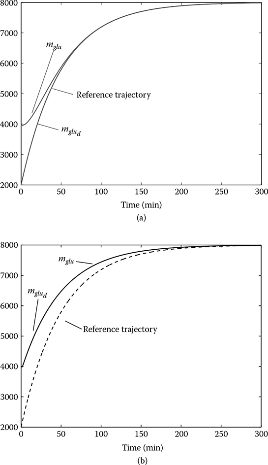
FIGURE 9.3
Tracking performances for time- driven control (a) and data- driven control (b), respectively.

Images

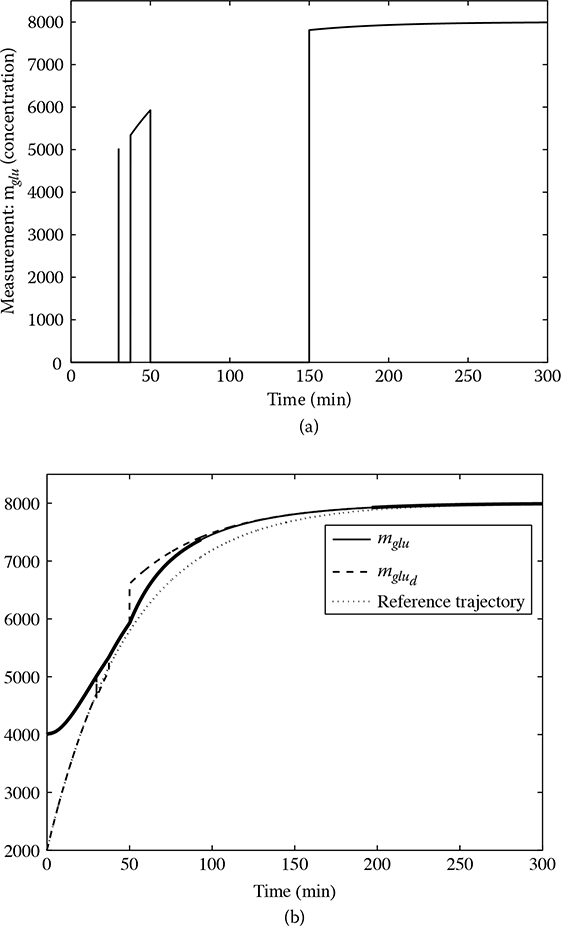
FIGURE 9.4
(a) Available measurement; (b) tracking performance.

Acknowledgment

This research was sponsored by the Office of Naval Research under award number ONR- N00014-11-1-0622. The authors are grateful for the support.

References

1. H. Kitano, “Systems biology: A brief overview,”Science, vol. 295, pp. 1662–1664, March 1, 2002.

2. M. Treuer, T. Weissbach, and V. Hagenmeyer, “Flatness- based feedforward in a two- degree- of- freedom control of a pumped storage power plant,” IEEE Transactions on Control Systems Technology, vol. 19, pp. 1540–1548, 2011.

3. L. Brus, T. Wigren, and D. Zambrano, “Feedforward model predictive control of a non- linear solar collector plant with varying delays,”Control Theory and Applications, IET, vol. 4, pp. 1421–1435, 2010.

4. Z. Hou and S. Jin, “A novel data-driven control approach for a class of discrete-time nonlinear systems,”IEEE Transactions on Control Systems Technology, vol. 19, pp. 1549–1558, 2011.

5. F. Previdi, T. Schauer, S. M. Savaresi, and K. J. Hunt, “Data- driven control design for neuroprotheses: A virtual reference feedback tuning (VRFT) approach,” Control Systems Technology, IEEE Transactions on, vol. 12, pp. 176–182, 2004.

6. M. Song, T. J. Tarn, and N. Xi, “Integration of task scheduling, action planning, and control in robotic manufacturing systems,”Proceedings of the IEEE, vol. 88, pp. 1097–1107, 2000.

7. G. M. Clayton, S. Tien, K. K. Leang, Q. Zou, and S. Devasia, “A review of feed-forward control approaches in nanopositioning for high-speed SPM,”Journal of Dynamic Systems, Measurement, and Control, vol. 131, pp. 061101–061119, 2009.

8. N. Xi and T. J. Tarn, “Stability analysis of non- time referenced Internet- based telerobotic systems,”Robotics and Autonomous Systems, vol. 32, pp. 173–178, 2000.

9. N. Xi, T.-J. Tarn, and A. K. Bejczy, “Intelligent planning and control for multirobot coordination: An event- based approach,”IEEE Transactions on Robotics and Automation, vol. 12, pp. 439–452, 1996.

10. S. Devasia, C. Degang, and B. Paden, “Nonlinear inversion- based output tracking,”IEEE Transactions on Automatic Control, vol. 41, pp. 930–942, 1996.

11. Z. Qingze and S. Devasia, “Preview- based optimal inversion for output tracking: Application to scanning tunneling microscopy,”IEEE Transactions on Control Systems Technology, vol. 12, pp. 375–386, 2004.

12. R. Yang, T.-J. Tarn, and M. Zhang, “Data- driven feedforward control for electro-poration mediated gene delivery in gene therapy,”IEEE Transactions on Control Systems Technology, vol. 18, pp. 935–943, 2010.

13. S. Bewick, R. Yang, and M. Zhang, “Complex mathematical models of biology at the nanoscale,”Wiley Interdisciplinary Reviews: Nanomedicine and Nanobiotechnology, vol. 1, pp. 650–659, 2009.

14. A. Isidori, Nonlinear Control Systems, Third Ed., Springer, London, 1995.

15. R. Yang, S. C. Lenaghan, J. P. Wikswo, and M. Zhang, “External control of the GAL network in S. cerevisiae: A view from control theory,”PLoS ONE, vol. 6, p. e19353, 2011.

16. M. R. Bennett, W. L. Pang, N. A. Ostroff, B. L. Baumgartner, S. Nayak, L. S. Tsimring, and J. Hasty, “Metabolic gene regulation in a dynamically changing environment,”Nature, vol. 454, pp. 1119–1122, 2008.

..................Content has been hidden....................

You can't read the all page of ebook, please click here login for view all page.

Table of Contents for
9 Hybrid Control for Micro/Nano Devices and Systems