7 Modeling Swimming Micro/Nano-Systems in Low Reynolds Number

When the concept of swimming is presented, we naturally envision a high Reynolds number environment, mostly because our environment is that of a high Reynolds number. In this environment, inertial forces dominate and must be overcome in order to produce movement. Bacteria and other microorganisms live in a low Reynolds number environment and are subject to different physical laws.

The Reynolds number is defined as

Re= \frac{ρ U L}{η} (7.1)

$Re= \frac{ρ U L}{η} (7.1)$

where U = the mean velocity of the object relative to the fluid, L = characteristic linear dimension, η= viscosity of the fluid, and ρ = density of the fluid. When Equation (7.1) is multiplied by vL/vL, it becomes [1]

Re= \frac{ρ U L}{η} = \frac{ρ v^{2} L 2}{η v L} = (Inertia forces) / (Viscous forces) (7.2)

$Re= \frac{ρ U L}{η} = \frac{ρ v^{2} L 2}{η v L} = (Inertia forces) / (Viscous forces) (7.2)$

In a low Reynolds number environment, the viscous forces dominate the inertial forces. This effect can be seen in Equation 7.2, and the fluid passively responds to external forces. This means that a nonzero force on an object results in infinite acceleration [2]. As a result, the total net force and torque of an object in a low Reynolds number is always zero. This means that the movement of the object at a given moment is totally determined by the force exerted on it at that moment, and by nothing in the past [3]. Reciprocal motion in this type of environment does not lead to any progress. For an incompressible fluid the Navier– Stokes equations govern fluid movements,

\begin{matrix} ρ (\frac{\partial}{\partial t} + u . Δ) u = - Δ p + η \nabla^{2} u, & \nabla \end{matrix} \cdot u = 0 (7.3)

$\begin{matrix} ρ (\frac{\partial}{\partial t} + u . Δ) u = - Δ p + η \nabla^{2} u, & \nabla \end{matrix} \cdot u = 0 (7.3)$

with u being the flow field of the fluid and p the pressure of the surrounding medium. In low Reynolds number situations, the equation can be simplified to the Stokes equation,

\begin{matrix} - \nabla p + μ \nabla^{2} v = 0, & \nabla \cdot u = 0 \end{matrix} (7.4)

$\begin{matrix} - \nabla p + μ \nabla^{2} v = 0, & \nabla \cdot u = 0 \end{matrix} (7.4)$

Speed does not impact the motion because Equation 7.4 is time independent, so only body movements have an effect on the motion. If the body motion involves reciprocal shapes, which makes the process time reversible, no advancement in position occurs [2].

Bacteria and other micro-swimmers have developed numerous strategies to maneuver and navigate through this sort of environment; for example, prokaryotic cells swim using flagella motility, gliding, and twitching motility, while eukaryotic bacteria swim using flagella, cilia, or pseudopodia.

7.2 Prokaryotic Cell Swimming Strategies

7.2.1 Prokaryotic Flagella

Prokaryotic flagella are filamentous helical protein structures used for swimming in aqueous environments. Swimming speeds vary greatly between species. Escherichia coli swim at a rate of 25–35 μm/s, while Bdellovibrio bacteriovorus can reach up to 160 μm/s [4]. The flagellum is made up of the basal body, filament, and hook. The basal body acts as a motor. The motor, a reversible one, converts energy into useful mechanical motion similar to the motor found in cars and other mechanical devices. The flagella filament is rotated by this motor thus allowing the cell to swim. The hook couples the filament and the basal body. The energy for rotation is received from the gradients of ions across the cytoplasmic membrane; these ions are either protons or sodium. The motor works similar to a turbine, driven by the flow of ions [5]. These motors are exceptionally fast and have been reported to have speeds of up to 100,000 rpm. The hook connects the basal body and the filament and acts as a universal joint [4]. Most prokaryotic flagella can rotate both counterclockwise and clockwise, which contributes to their ability to change direction during swimming.

7.2.2 Twitching Motility

Twitching motility is a form of bacteria motility over moist surfaces that is independent of the use of the flagella. It occurs by extension, tethering, and then retraction of polar type IV pili, which operate in a manner similar to a grappling hook. It is mediated by type IV pili located at one or both poles of the cell and differs from flagella motility, which is mediated by the rotation of unipolar flagella [6]. Twitching motility is controlled by an array of signal transduction systems, including two- component sensor- regulators and a chemosensory system [6].

This type of motion was coined “twitching” because when it was first discovered in 1961, the cells appeared to move in a jerky fashion that resembled twitching [7].

Twitching motility is used by a wide range of bacteria, the best studied of which are Pseudomonas aeruginosa, Neisseria gonorrhoeae, and Myxococcus xanthus, where it is referred to as “social gliding motility” [6].

Twitching motility is used predominantly as a means for bacteria to travel in a low water content environment and to colonize hydrated surfaces, as opposed to free living in fluids [6]. It is vital for colonial behaviors such as the formation of biofilms and fruiting bodies [8].

7.2.3 Gliding Motility

Gliding motility is defined as a smooth translocation of cells over a surface by an active process that requires the expenditure of energy. It is flagella independent and follows the long axis of the cell [9]. Gliding bacteria live in environments as diverse as the human mouth, ocean sediments, and garden soil.

Studies have shown that gliding motility cannot be explained by a single mechanism. It appears that several different types of motors have evolved that allow movement over surfaces; some bacteria use type IV pilus extension and retraction, possibly powered by ATP hydrolysis, to propel themselves [9]. This process is sometimes put into the category of twitching motility, and it is a matter of debate if this system of motion should be considered twitching or gliding. Twitching is normally used to describe discontinuous cell movements, while gliding is used to describe smooth, continuous movements. A source for further confusion is that an organism that appears to twitch under certain conditions might appear to glide under other conditions [9]. Other forms of gliding that do not use pili exist. One example is mycoplasmas that depend on their well- developed cytoskeleton and surface adhesion proteins to crawl over surfaces. Some filamentous cyanobacteria’s gliding motility may be powered by polysaccharide extrusion [9].

7.3 Eukaryotic Cell Swimming Strategies

7.3.1 Eukaryotic Flagella

Eukaryotic flagella are whiplike appendages that have a “9 + 2” structure, which is referred to as the axoneme; it has nine pairs of microtubule doublets surrounding two central single microtubules. At the base, it has a basal body that is the microtubule organizing center. The outer nine doublet microtubules extend a pair of dynein arms to the neighboring microtubule. The dynein arms cause flagella beating; through ATP hydrolysis, a force is produced by the dynein arms and results in the microtubule doublets sliding against each other and the whole flagellum bending. This mechanism is unlike the prokaryotic flagella working by a motor rotating the flagella. The eukaryotic flagella motion is usually planar and in the form of a traveling sinusoidal wave.

As an example of how the swimming of eukaryotic flagellum can be modeled, we will present an overview of the local resistive force theory and use it to understand Gray and Hancock’s work on the propulsion of the sea urchin spermatozoa [10]. In order to model swimming in low Reynolds number situations, Equation 7.4, Stokes’ equation, must be solved. Using Green’s function for Stokes flow with a dirac-delta forcing of the form δ(x – x′)F, the fundamental solution to Stokes’ equation is

u (x) = G (x - x^{'}) \cdot F (7.5)

$u (x) = G (x - x^{'}) \cdot F (7.5)$

The Oseen tensor (G tensor) is

G (r) = \frac{1}{8 π η} (\frac{1}{| r |} + \frac{| r | r |}{r |^{3}}) (7.6)

$G (r) = \frac{1}{8 π η} (\frac{1}{| r |} + \frac{| r | r |}{r |^{3}}) (7.6)$

Equations (7.5) and (7.6) are referred to as a stokeslet, which represents a flow field due to F, a point force acting on the fluid at the position x′ as a singularity [11]. To better understand the local drag theory we will use a representative model by Lauga and Powers [11]. The goal of the model is to find an approximate form for the resistance matrix of the flagella with errors controlled by the small parameter a/L, with a as the radius and L as the length [11]. The model assumes the flagellum to be a rod with length L and radius a subjected to an external force F_ext (uniformly distributed over the length of the rod); the rod is divided into equally spaced N points along the x-axis with the positions x_j = (jL/N, 0, 0). These points are considered to be stokeslets, the far field flow induced by a short segment of the rod [11]. The velocity of each segment of the rod without taking into consideration the effects of other segments on it is u = F_ext/ξ_seg, where ξ_seg∝ηa is the resistance coefficient of a segment. But since the flow induced by a segment affects all the other segments as well, the hydrodynamic interactions of the segments have to be included. The velocity of a segment u_j as a result of the j th segment is

u_{i} (x) = \frac{1}{8 π η | x - x_{j} |} (1 + e_{x} e_{x}) \cdot [\frac{F_{e x t}}{N}] (7.7)

$u_{i} (x) = \frac{1}{8 π η | x - x_{j} |} (1 + e_{x} e_{x}) \cdot [\frac{F_{e x t}}{N}] (7.7)$

So the velocity of a segment (ith segment) is a combination of the flows resulting from other segments and its velocity without the consideration of other segments,

u (x_{i}) = \frac{F_{e x t}}{ξ_{s e g}} + Σ_{j \neq i} u_{j} (x_{i}) (7.8)

$u (x_{i}) = \frac{F_{e x t}}{ξ_{s e g}} + Σ_{j \neq i} u_{j} (x_{i}) (7.8)$

The sum over i is replaced by an integral taking into account that the density of the spheres is L/ N and excluding a small region around x_i from the region of integration. This results in

u (x_{i}) = \frac{F_{e x t}}{ξ_{s e g}} + \frac{1}{8 π η} \int^{'} \frac{1}{| x_{i} - x |} (1 + e_{x} e_{x}) \cdot F_{e x t} \frac{d x}{L} (7.9)

$u (x_{i}) = \frac{F_{e x t}}{ξ_{s e g}} + \frac{1}{8 π η} \int^{'} \frac{1}{| x_{i} - x |} (1 + e_{x} e_{x}) \cdot F_{e x t} \frac{d x}{L} (7.9)$

The prime above the integral signifies that the region of integration is between −L/2 to L/2 except for a region with size order a around x_i. With the end effects disregarded because |x_i| << L, the preceding Equation 7.9 becomes

u (x_{i}) = \frac{F_{e x t}}{ξ_{s e g}} + \frac{1}{4 π η} \ln (\frac{L}{4 a}) (1_{e_{x} e_{x}}) \cdot (\frac{F_{e x t}}{L}) (7.10)

$u (x_{i}) = \frac{F_{e x t}}{ξ_{s e g}} + \frac{1}{4 π η} \ln (\frac{L}{4 a}) (1_{e_{x} e_{x}}) \cdot (\frac{F_{e x t}}{L}) (7.10)$

Keeping only the terms that are leading orders in (L/a) and using the fact that u(x_i) is constant for a rigid rod, the equation becomes

u = \frac{\ln (L / a)}{4 π η} (1 + e_{x} e_{x}) \cdot (\frac{F_{e x t}}{L}) (7.11)

$u = \frac{\ln (L / a)}{4 π η} (1 + e_{x} e_{x}) \cdot (\frac{F_{e x t}}{L}) (7.11)$

An assumption of the model is that there is no internal cohesive force acting between any pair of segments; only the hydrodynamic force is present. So the drag per unit length is f = –F_ext/L and

\begin{matrix} f_{N} = - ξ_{N} u_{N,} f_{T} = - ξ_{T} u_{T} \\ ξ_{N} = 2 ξ_{T} = 4 π η / \ln (L / a) \end{matrix} (7.12)

$\begin{matrix} f_{N} = - ξ_{N} u_{N,} f_{T} = - ξ_{T} u_{T} \\ ξ_{N} = 2 ξ_{T} = 4 π η / \ln (L / a) \end{matrix} (7.12)$

with N and T expressing the components normal and tangential to the x-axis. The movement of a thin filament in a viscous fluid elicits resistive forces in the normal and tangential directions of motion; an example of this phenomenon is illustrated in Figure 7.1.

Images

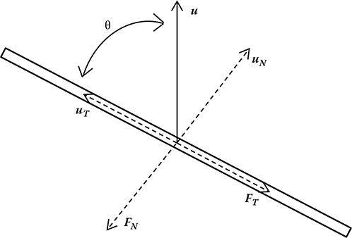
FIGURE 7.1
Representation of drag experienced by a slender body in a viscous fluid moving at a velocity u (see text for notation).

The resistive force theory does have its limitations. Lauga and Powers [11] use the example of the sedimentation rate of a ring in a highly viscous fluid of radius R and rod diameter 2a (plane is horizontal) versus a straight rod of length L= 2piR [11]. Even though the length of both rods is the same, the ring should fall faster because the segments of the ring are closer together, but using the drag coefficients of Equation 7.12 would have both falling at the same rate. This is because the above derivation assumes zero deformation in the filament. In filaments with a small curvature, it is assumed that the viscous force per unit length is the same as a rigid rod of the same length. So the theory does not take into account the significant curvature of the ring. A way to improve this theory is to implement a combination of a smooth distribution of stokeslets and source dipoles to make a better approximation for the flow induced by the motion of the rod [11]. Gray and Hancock (henceforth referred to as G– H) used this approach to a sine wave with wavelength λ and derived the following equations for the resistive coefficients [10,12]

ξ_{N} = 2 ξ_{T} = \frac{4 π η}{n (2 λ / a) - \frac{1}{2}} (7.13)

$ξ_{N} = 2 ξ_{T} = \frac{4 π η}{n (2 λ / a) - \frac{1}{2}} (7.13)$

G– H implemented this to analyze the propulsion of sea urchin spermatozoa. Their findings, recorded in the paper titled “The Propulsion of Sea Urchin Spermatozoa” [10], have since served as a basis for further work in flagellated microorganism propulsion studies.

The paper’s objective was to investigate the forces the surrounding medium applied on the flagellum as the whole sperm swam and to relate the propulsive speed of the whole sperm to the form and speed of propagation of the bending waves generated by the tail. A spermatozoan’s propulsion relies on the fact that the propulsive forces acting normally to the surface of the body offset the retarding tangential forces acting along the body. G– H use the forces elicited from the transverse displacement (V_y) impacted on a short element (δs) during the passage of a wave (Figure 7.2).V_y has two components: the tangential displacement V_y sin(θ), and the displacement normal to the surface of the element V_y cos(θ). The surrounding medium acts as a retarding force to both these displacements and as a result V_y causes reactions normal to the tangential and normal to the surface of the element similar to the phenomenon in Figure 7.1. The component of the force δN_y that acts along the axis of propulsion (δN_y sin(θ)) counteracts the retarding effect of all the forces acting tangentially to the surface.

Since dimensions of an element are minuscule and the displacement speed low, the reactions from the medium can be assumed to be directly proportional to the velocity of displacement, and to the viscosity of the medium. The velocity of displacement tangential to the body is V_y sin(θ), the tangential drag (δL_y) isξ_TV_y sin(θ)δs, and the normal force (δN_y) to the surface is ξ_NV_y cos(θ)δs.ξ_T and ξ_N are the drag coefficients of Equation 7.13. The resultant forward thrust (δF_y) along the axis of propulsion is (ξ_N –ξ_T)V_y sin θcos θδs. This equation shows that the only way the displacement of the element will result in a forward thrust in the axis of propulsion is if ξ_N > ξ_T. The sperm is moving not only transversely across the axis of propulsion but also along the latter axis at V_x, which is dependent on how the entire sperm is moving through the medium. V_x also has two components: the tangential displacement V_x cos(θ), and the displacement normal to the surface of the element V_x sin(θ), which results in the forces acting tangentially and normally to the surface (δL_x and δN_x, respectively). δL_x = ξ_TV_x cos(θ)δs, andδN_x = ξ_NV_x sin(θ)δs.

Images

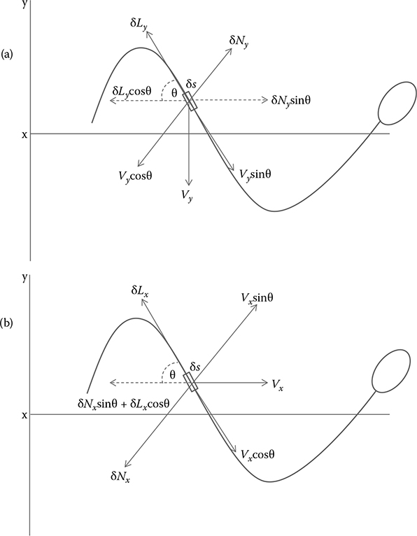
FIGURE 7.2
Representation of Gray and Hancock’s swimming sea urchin spermatozoa. (a) Forces impressed on an element δs moving transversely with a velocity of V_y; (b) Forces impressed on the elementδs when swimming along the x axis with a velocity of V_x.

The total forces acting on the surface because of the elements’ transverse and forward displacements are

\begin{matrix} δ N = ξ_{N} (V_{y} \cos (θ) - V_{x} \sin (θ)) δ s, & δ L = ξ_{T} (V_{y} \sin (θ) + V_{x} \cos (θ)) δ s \end{matrix} (7.14)

$\begin{matrix} δ N = ξ_{N} (V_{y} \cos (θ) - V_{x} \sin (θ)) δ s, & δ L = ξ_{T} (V_{y} \sin (θ) + V_{x} \cos (θ)) δ s \end{matrix} (7.14)$

The resultant forward thrust is

δ F = δ N sin θ - δ L \cos θ (7.15)

$δ F = δ N sin θ - δ L \cos θ (7.15)$

since the propulsive components of δN and δL are δN sin θ and δL cos θ, respectively. So

\begin{matrix} δ F & = & [(ξ_{N} - ξ_{T}) V_{y} \sin θ \cos θ - V_{x} (ξ_{N} \sin^{2} θ + ξ_{T} C o s^{2} θ)] δ s \\ = & [((ξ_{N} - ξ_{T}) V_{y} \tan θ - V_{x} \tan θ - V_{x} (ξ_{T} + ξ_{N} \tan^{2} θ)) / (1 + \tan^{2} θ)] δ s \end{matrix} (7.16)

$\begin{matrix} δ F & = & [(ξ_{N} - ξ_{T}) V_{y} \sin θ \cos θ - V_{x} (ξ_{N} \sin^{2} θ + ξ_{T} C o s^{2} θ)] δ s \\ = & [((ξ_{N} - ξ_{T}) V_{y} \tan θ - V_{x} \tan θ - V_{x} (ξ_{T} + ξ_{N} \tan^{2} θ)) / (1 + \tan^{2} θ)] δ s \end{matrix} (7.16)$

From Equation 7.14, we can see that a forward thrust is possible only if V_y > V_x tanθ and Equation 7.16 shows that the forward thrust happens only if ξ_N > ξ_T. Now the propulsive speed can be expressed in terms of the wave speed as long as the propulsive speed remains constant during the whole cycle of the element’s motion. The above principles can be applied to an undulating filament driving an inert head by setting the transverse velocity of an element (δs) to dy/ dt. The tangent of its angle of inclination is dy/ dx, so Equation 7.16 becomes

d F = [((ξ_{N} - ξ_{T})) \frac{d y}{d t} \frac{d y}{d x} - V_{x} (ξ_{T} + ξ_{N} (\frac{d y}{d x})^{2}) / (1 + {(\frac{d y}{d x})}^{2})] δ s (7.17)

$d F = [((ξ_{N} - ξ_{T})) \frac{d y}{d t} \frac{d y}{d x} - V_{x} (ξ_{T} + ξ_{N} (\frac{d y}{d x})^{2}) / (1 + {(\frac{d y}{d x})}^{2})] δ s (7.17)$

The total force along the length of the flagellum over one wavelength is

F = \int_{0}^{λ} d F (7.18)

$F = \int_{0}^{λ} d F (7.18)$

The equation for a filament propelling an inert head is

n \int_{0}^{λ} d F - ξ_{H} \bar{V_{x}} = 0 (7.19)

$n \int_{0}^{λ} d F - ξ_{H} \bar{V_{x}} = 0 (7.19)$

with $\bar{V_{x}}$ $\bar{V_{x}}$ being the average velocity of forward propulsion over a complete cycle of activity, ξ_H is the drag coefficient of the head (for a sphere ξ_H = 6πaη, with a being the radius of the sphere and η being the viscosity of the medium), and n is the number of waves exhibited by the whole tail.

This work has served as a basis for further work in flagellated microorganism propulsion studies. Lighthill [13] has conducted further analysis on this problem and provided more accurate values for ξ_N and ξ_T. Even though there are still limitations to the local drag theory, it has been shown to be useful for calculating and predicting characteristics of flagella- based propulsion of microorganisms. The local drag theory has since been expanded upon by using the slender body theory for a more accurate analysis.

7.3.2 Cilia

Similar to the eukaryotic flagellum, cilia consist of a “9 + 2” structure but are shorter than the flagella. Eukaryotic flagella and cilia are structurally identical and the distinctions between them are often made based on their function and length. Together cilia and flagella are known as a group of organelles called undulipodia[14,15]. The motile cilia enable cells to move by moving liquid past the surface of the cell. The cause of cilia movement is similar to that of the eukaryotic flagella; ATP hydrolysis creates forces in the dynein arms that cause the structure to bend. Unlike eukaryotic flagella, cilia perform 3D motion and consist of a power and recovery stroke [16].

7.3.3 Pseudopodia

The next swimming strategy for eukaryotes to be discussed is the pseudopodia mechanism. Pseudopodia are temporary extensions of eukaryotic cell cytoplasm. They are used by sarcodine protozoans, some flagellated protozoans, some cells of animals, and amoeba as a means of locomotion. They extend and contract by the reversible assembly of actin subunits into microfilaments; projections occur when there is an interaction between myosin and filaments near the cell’s end [17]. The projections continue until actin reassembles into a network. In the case of amoeba, the amoeba extends multiple pseudopodia and then drags itself toward the direction of one of them. Four of the best known types of pseudopodia are axopodia, filopodia, lamellipodia, and reticulopodia. Axopodia are characteristically stiff, slender, and have internal rods consisting of an array of microtubules. Filopodia are also slender but do not have microtubules (in most protists); instead, they contain actin filaments. The lamellipodia, which are characteristic of Amoeba, are broad flat protrusions, and reticulopodia are slender and anastomosing pseudopodia that form a cross-connecting net that is stiffened by both microtubules and filaments [18].

7.4 Dynamics Modeling and Analysis of a Swimming Microrobot for Controlled Drug Delivery

This section discusses possible design and control of a swimming microrobot. We specifically use the work of Li, Tan, and Zhang in their “Dynamics Modeling and Analysis of a Swimming Microrobot for Controlled Drug Delivery” [19,20]. In the paper, a swimming robot composed of a spiral type head and an elastic tail modeled with the resistive force theory previously discussed is proposed. The microrobot is designed for optimal drug delivery, and thus suitable for low Reynolds number swimming. External rotating magnetic fields drive the head of the swimming robot, which allows it to be remotely controlled wirelessly. The head serves as a base for the elastic tail and houses the communication and control units. When a rotating magnetic field is applied, the head rotates in unison with the field, and a driving torque is propagated to the straight elastic tail. Deformation of the tail occurs when a threshold level of the driving torque is reached resulting in the tail transforming into a helix, and generating propulsive thrust. The tail also serves as a drug reservoir in controlled drug delivery operations.

The modeling and analysis of the microrobot were split into analysis before and after the bifurcation of the tail. Bifurcation is the remarkable deformation of rotating filaments [20]. Li et al.’s previous studies had shown that applying increasing driving torque to straight elastic polymers that are clamped at one end and open at the other results in a strongly discontinuous shape deformation at a finite torque (N_C) and a finite rotation frequency (ω_C). In order for significant propulsion to be achieved, the driving torque or rotation frequency has to reach the above thresholds (N_C and ω_C).

7.4.1 Before Bifurcation

Prior to the deformation, the tail is relatively straight and propulsion is negligible, and the tail can be regarded as pure payload [20]. For the entire system to rotate the viscous friction resulting from the head and tail has to be overcome by the driving torque. The resistive torque (T_R) equation is

T_{R} = T_{H} + T_{T} (7.20)

$T_{R} = T_{H} + T_{T} (7.20)$

T_H and T_T are resistive torques from the head and tail, respectively. T_H is then decomposed into

T_{H} = T_{P + T_{S}} (7.21)

$T_{H} = T_{P + T_{S}} (7.21)$

T_P is the resistive torque of the payload, while T_S is the resistive torque from the spiral head. So the moment balance equation of the microrobot is

T_{D} + T_{T} + T_{P} + T_{S} = 0 (7.22)

$T_{D} + T_{T} + T_{P} + T_{S} = 0 (7.22)$

T_D is the driving torque on the head from the external magnetic field, and it is represented as

T_{D} = m H \sin β (7.23)

$T_{D} = m H \sin β (7.23)$

where m is the magnetized moment of the magnetized head, H is the magnetic field’s amplitude, and β is the angle between them. The payload in the head is modeled as a sphere with radius d. The resistive torque of a sphere according to Stokes’ law is

T_{P} = D_{R} ω (7.24)

$T_{P} = D_{R} ω (7.24)$

with D_R a sphere’s rotational drag coefficient,

D_{R} = 8 π η d^{3} (7.25)

$D_{R} = 8 π η d^{3} (7.25)$

where d is as the radius of the sphere. The tail is modeled as an elongated rod, so the axial rotational resistance torque can be represented as

T_{T} = E_{R} L_{T b} ω (7.26)

$T_{T} = E_{R} L_{T b} ω (7.26)$

where L_Tb is the length of the tail before bifurcation, ω is the swimming velocity of the microrobot, and E_R is the rotational resistance of an elongated rod

E_{R} = 4 π μ η d^{2} (7.27)

$E_{R} = 4 π μ η d^{2} (7.27)$

a_S is the cross-sectional radius of the elastic tail.

The viscous force per length along the y direction due to the spiral head is assumed to be F_Y. So T_S is represented by

T_{s} = A_{H} F_{γ} L_{H} (7.28)

$T_{s} = A_{H} F_{γ} L_{H} (7.28)$

where A_H is the helical amplitude of the head and L_H is the length of the head. So the moment balance equation from Equation 7.22 can be rewritten as

T_{D} + E_{R} L_{T b} ω + D_{R} ω + A_{H} F_{γ} L_{H} = 0 (7.29)

$T_{D} + E_{R} L_{T b} ω + D_{R} ω + A_{H} F_{γ} L_{H} = 0 (7.29)$

Similarly, the force balance equation is

F_{T} + F_{P} + F_{S} = 0 (7.30)

$F_{T} + F_{P} + F_{S} = 0 (7.30)$

where F_T is the translational resistive force brought by the circular tail, F_P is the translational resistive force brought by the payload, and F_S is the translational resistive force brought by the head itself.

Since the elastic tail is treated as an elongated rod before bifurcation, F_T can be obtained from

F_{T} = E_{L} V (7.31)

$F_{T} = E_{L} V (7.31)$

where V is the velocity of the microrobot, and E_L is the translational resistance of the elastic tail, and according to [21]

E_{L} = \frac{2 π η L_{T b}}{\ln (\frac{L_{T b}}{2 a_{b}}) + \ln 2 - \frac{1}{2}} (7.32)

$E_{L} = \frac{2 π η L_{T b}}{\ln (\frac{L_{T b}}{2 a_{b}}) + \ln 2 - \frac{1}{2}} (7.32)$

Next, F_P is defined as

F_{P} = D_{L} V (7.33)

$F_{P} = D_{L} V (7.33)$

where D_L is the translational drag coefficient of a sphere,

D_{L} = 6 π η d (7.34)

$D_{L} = 6 π η d (7.34)$

The viscous force per length along the x direction due to the spiral head is assumed to be F_X. So F_S is represented by

F_{S} = F_{X} L_{H} (7.35)

$F_{S} = F_{X} L_{H} (7.35)$

Therefore, the translational force balance equation is

E_{L} V + D_{L} V + F_{X} L_{H} = 0 (7.36)

$E_{L} V + D_{L} V + F_{X} L_{H} = 0 (7.36)$

The paper uses resistive force theory (RFT) to approximate F_X and F_Y as long as the radius of the microrobot body is extremely small compared to other relevant lengths.

ξ_L and ξ_N are given by [22]:

ξ_{T} = \frac{2 π η}{(\ln (\frac{2 P_{H}}{b} - 2.90))}, ξ_{N} = \frac{4 π η}{(\ln (\frac{2 P_{H}}{b}) - 1.90)} (7.37)

$ξ_{T} = \frac{2 π η}{(\ln (\frac{2 P_{H}}{b} - 2.90))}, ξ_{N} = \frac{4 π η}{(\ln (\frac{2 P_{H}}{b}) - 1.90)} (7.37)$

where b is the cross- sectional radius of the wire of the helical head, and P_H is the pitch of the helical head. The local velocities are decomposed into tangential and normal velocities; the relationships between velocities and forces along these directions are

F_{L} = ξ_{T} (ω A \sin θ - V \cos θ), F_{N} = ξ_{N} (ω A \cos θ + V \sin θ) (7.38)

$F_{L} = ξ_{T} (ω A \sin θ - V \cos θ), F_{N} = ξ_{N} (ω A \cos θ + V \sin θ) (7.38)$

where F_L and F_N are the tangential and normal forces, respectively. θ is defined as

\tan θ = 2 π A_{H} / P_{H} (7.39)

$\tan θ = 2 π A_{H} / P_{H} (7.39)$

The forces along the x and y directions are represented by F_L and F_N:

F_{X} = F_{L} \cos θ - F_{N} \sin θ, F_{γ} = F_{L} \sin θ + F_{N} \cos θ (7.40)

$F_{X} = F_{L} \cos θ - F_{N} \sin θ, F_{γ} = F_{L} \sin θ + F_{N} \cos θ (7.40)$

The translational velocity of the microrobot can be solved by combining Equations 7.36–7.40 into

V = \frac{ω A_{H} L_{H} \sin θ \cos θ (ξ_{N} - ξ_{T})}{D_{L} + E_{L} - L_{H} (ξ_{N} \sin^{2} θ + ξ_{T} \cos^{2} θ)} (7.41)

$V = \frac{ω A_{H} L_{H} \sin θ \cos θ (ξ_{N} - ξ_{T})}{D_{L} + E_{L} - L_{H} (ξ_{N} \sin^{2} θ + ξ_{T} \cos^{2} θ)} (7.41)$

The force along the x direction is

F_{X} = - V (E_{L} + D_{L}) / (L_{H}) = \frac{ω A_{H} \sin θ \cos θ (ξ_{T} - ξ_{N}) (D_{L} + E_{L})}{D_{L} + E_{L} - L_{H} (ξ_{N} \sin^{2} θ + ξ_{T} \cos^{2} θ)} (7.42)

$F_{X} = - V (E_{L} + D_{L}) / (L_{H}) = \frac{ω A_{H} \sin θ \cos θ (ξ_{T} - ξ_{N}) (D_{L} + E_{L})}{D_{L} + E_{L} - L_{H} (ξ_{N} \sin^{2} θ + ξ_{T} \cos^{2} θ)} (7.42)$

And the angular velocity of the microrobot is

ω = - \frac{T_{D}}{\frac{A_{H}^{2} L_{H}^{2} \sin^{2} θ \cos^{2} θ (ξ_{N} - ξ_{T})^{2}}{D_{L} + E_{L} - E_{H} (ξ_{N} \sin^{2} θ + ξ_{T} \cos^{2} θ)}} (7.43)

$ω = - \frac{T_{D}}{\frac{A_{H}^{2} L_{H}^{2} \sin^{2} θ \cos^{2} θ (ξ_{N} - ξ_{T})^{2}}{D_{L} + E_{L} - E_{H} (ξ_{N} \sin^{2} θ + ξ_{T} \cos^{2} θ)}} (7.43)$

where $S = E_{R} L_{T b} + D_{R} + A_{H}^{2} L_{H} (ξ_{T} \sin^{2} θ + ξ_{T} \cos^{2} θ)$ $S = E_{R} L_{T b} + D_{R} + A_{H}^{2} L_{H} (ξ_{T} \sin^{2} θ + ξ_{T} \cos^{2} θ)$

The system has zero total moment because the driving torque is balanced by the resistive torque from the head and the tail.

7.4.2 After Bifurcation

The elastic tail is assumed to be a circular cylinder with two geometric quantities, radius a and contour length L_Tb, and two material quantities: the bending modulus B and twist modulus T. The twist behavior was ignored because it does not directly relate to the bifurcation. Before bifurcation, the angular velocity ω of the microrobot is proportional to the driving torque. When ω is low, the tail remains straight while twisting along its centerline. When ω reaches its bifurcation frequency, the straight elastic tail shape turns into a helix. The bifurcation frequency of the tail is

ω_{c} = \frac{B}{E_{R} (L_{T b})^{2}} (7.44)

$ω_{c} = \frac{B}{E_{R} (L_{T b})^{2}} (7.44)$

When B is larger, the tail is stiffer and more resistant to bending; when E_R and L_Tb are larger, the tail experiences greater friction from the fluid and makes the tail easier to bend.

The torque and force balance Equations 7.22 and 7.30 still hold after bifurcation with one exception: the tail is no longer just payload but is a propulsive unit. The balance equations are

T_{D} + A_{T} F_{γ}^{*} L_{T a} + D_{R} ω + A_{H} F_{γ} L_{H} = 0 (7.45)

$T_{D} + A_{T} F_{γ}^{*} L_{T a} + D_{R} ω + A_{H} F_{γ} L_{H} = 0 (7.45)$

F_{X}^{*} L_{T a} + D_{L} V + F_{X} L_{H} = 0 (7.46)

$F_{X}^{*} L_{T a} + D_{L} V + F_{X} L_{H} = 0 (7.46)$

A_T is the amplitude of the tail after bifurcation, L_Ta is the length of the tail after bifurcation, F_X^* and F_Y^* and are the viscous force per unit length in the x and y directions due to the elastic tail. V and ω are related by

V = P ω (7.47)

$V = P ω (7.47)$

where

\begin{matrix} P & = & \frac{M + M *}{D_{L} - N - N^{*}} \\ M & = & A_{H} L_{H} \sin θ \cos θ (ξ_{N} - ξ_{T}) \\ N & = & L_{H} (ξ_{N} \sin^{2} θ + ξ_{T} \cos^{2} θ) \\ M^{*} & = & A_{T} L_{T a} \sin θ^{*} \cos^{*} (ξ_{N}^{*} - ξ_{T}^{*}) \\ N^{*} & = & L_{T a} ξ_{N}^{*} \sin^{2} θ^{*} \\ ξ_{T}^{*} & = & \frac{2 π η}{(\ln (\frac{2 P_{T}}{a}) - 2.90)}, ξ_{N}^{*} = \frac{4 π η}{(\ln (\frac{2 P_{T}}{a}) - 1.90)}, \end{matrix}

$\begin{matrix} P & = & \frac{M + M *}{D_{L} - N - N^{*}} \\ M & = & A_{H} L_{H} \sin θ \cos θ (ξ_{N} - ξ_{T}) \\ N & = & L_{H} (ξ_{N} \sin^{2} θ + ξ_{T} \cos^{2} θ) \\ M^{*} & = & A_{T} L_{T a} \sin θ^{*} \cos^{*} (ξ_{N}^{*} - ξ_{T}^{*}) \\ N^{*} & = & L_{T a} ξ_{N}^{*} \sin^{2} θ^{*} \\ ξ_{T}^{*} & = & \frac{2 π η}{(\ln (\frac{2 P_{T}}{a}) - 2.90)}, ξ_{N}^{*} = \frac{4 π η}{(\ln (\frac{2 P_{T}}{a}) - 1.90)}, \end{matrix}$

P_T is the pitch of the helical tail, A_T is the amplitude, and L_Ta is the length. The asterisk denotes components of the tail after bifurcation. F_Y and F_Y^* in Equation 7.45can be represented as Qω and Q^*ω, respectively.

\begin{matrix} Q & = & A_{H} (ξ_{T} \sin^{2} θ) + P \sin θ \cos θ ({ξ_{N} - ξ}_{T}) \\ Q^{*} & = & A_{T} (ξ_{T}^{*} \sin^{2} θ^{*}) + P \sin θ^{*} \cos θ^{*} (ξ_{N}^{*} - ξ_{T}^{*}) \end{matrix}

$\begin{matrix} Q & = & A_{H} (ξ_{T} \sin^{2} θ) + P \sin θ \cos θ ({ξ_{N} - ξ}_{T}) \\ Q^{*} & = & A_{T} (ξ_{T}^{*} \sin^{2} θ^{*}) + P \sin θ^{*} \cos θ^{*} (ξ_{N}^{*} - ξ_{T}^{*}) \end{matrix}$

Substituting F_Y and F_Y^* into Equation 7.45, the angular velocity can be written as

ω = - \frac{T_{D}}{A_{T} L_{T a} Q^{*} + A_{H} L_{H} Q + D_{R}} (7.48)

$ω = - \frac{T_{D}}{A_{T} L_{T a} Q^{*} + A_{H} L_{H} Q + D_{R}} (7.48)$

Through simulations, the preceding model of a microrobot was shown to be able to move more freely in a constrained area due to the flexible dimensions and was more efficient when compared to a rigid body spiral- type microrobot [20]. Li et al. also asserted that the elastic tail could lead to easier formation of a flagella bundle which in turn would produce greater thrusts than a single one. Also, because the tail is not just pure payload, it helps generate additional thrust and increase the energy efficiency of the microrobot. Li et al. proposed that this design could be used for a wide range of medical applications.

Acknowledgment

The authors are grateful for the support of the Office of Naval Research under award number ONR- N00014-11-1-0622.

References

1. Batchelor, G.K. An Introduction to Fluid Dynamics. Cambridge, UK: Cambridge University Press, pp. 211–215.

2. Cohen, N. and J.H. Boyle, Swimming at low Reynolds number: A beginners guide to undulatory locomotion. Contemporary Physics, 2010,51(2): pp. 103–123.

3. Purcell, E.M. Life at low Reynolds number.American Journal of Physics, 1977, 45(1): pp. 3–11.

4. Jarrell, K.F. and M.J. McBride. The surprisingly diverse ways that prokaryotes move. Nature Reviews Microbiology, 2008,6(6): pp. 466–476.

5. Blair, D.F. and S.K. Dutcher. Flagella in prokaryotes and lower eukaryotes. Current Opinion in Genetics and Development, 1992,2(5): pp. 756–767.

6. Mattick, J.S. Type IV pili and twitching motility.Annual Review of Microbiology, 2002,56: pp. 289–314.

7. Henrichsen, J. Twitching motility. Annual Review of Microbiology, 1983,37: pp. 81–93.

8. O’Toole, G.A. and R. Kolter. Flagellar and twitching motility are necessary for Pseudomonas aeruginosa biofilm development.Molecular Microbiology, 1998, 30(2): pp. 295–304.

9. Mcbride, M.J. Bacterial gliding motility: Multiple mechanisms for cell movement over surfaces. Annual Review of Microbiology, 2001, 55: pp. 49–75.

10. Gray, J. and G.J. Hancock. The propulsion of sea-urchin spermatozoa. Journal of Experimental Biology, 1955,32: pp. 802–814.

11. Lauga, E. and T.R. Powers. The Hydrodynamics of Swimming Microorganisms. Reports on Progress in Physics, 2009, 72(9) 096601.

12. Hancock, G.J. The self- propulsion of microscopic organisms through liquids Proceedings of the Royal Society of London Series Mathematical and Physical Sciences, 1953. 217(1128): pp. 96–121.

13. Lighthill, J. Flagellar Hydrodynamics: The John von Neumann Lecture, 1975. SIAM Review, 1976. 18(2): pp. 161–230.

14. Gibbons, I.R. Cilia and flagella of eukaryotes. Journal of Cell Biology, 1981. 91(3): pp. S107–S124.

15. Margulis, L. Undulipodia, flagella and cilia.Biosystems, 1980.12(1–2): pp. 105–108.

16. Walczak, C.E. and D.L. Nelson. Regulation of dynein-driven motility in cilia and flagella. Cell Motility and the Cytoskeleton, 1994.27(2): pp. 101–107.

17. Sadava, D.E.Life: The Science of Biology 2011, Sunderland, MA: Sinauer Associates.

18. Davidovich, N.A. et al. Mechanism of male gamete motility in araphid pen-nate diatoms from the genus Tabularia (Bacillariophyta). Protist, 2012, 163(3): pp. 480–494.

19. Huaming, L., T. Jindong, and Z. Mingjun. Dynamics modeling and analysis of a swimming microrobot for controlled drug delivery. In ICRA 2006. Proceedings 2006 IEEE International Conference on Robotics and Automation.

20. Li, H.M., J.D. Tan, and M.J. Zhang. Dynamics modeling and analysis of a swimming microrobot for controlled drug delivery. IEEE Transactions on Automation Science and Engineering, 2009, 6(2): pp. 220–227.

21. Lighthill, J.S.Mathematical Biofluiddynamics, 1975, Philadelphia: Society for Industrial and Applied Mathematics.

22. Nakano, M., S. Tsutsumi, and H. Fukunaga. Magnetic properties of Nd- Fe- B thick- film magnets prepared by laser ablation technique. IEEE Transactions on Magnetics, 2002, 38(5): pp. 2913–2915.

..................Content has been hidden....................

You can't read the all page of ebook, please click here login for view all page.

Table of Contents for
7 Modeling Swimming Micro/Nano-Systems in Low Reynolds Number