Table Basics

Tables are the sine qua non of spreadsheet applications, so it’s important that you understand the basics of table handling, whether you’ve never used a spreadsheet program or are accustomed to the Excel or Google Sheets approach where table=spreadsheet=table.

In this chapter, we start with Numbers’ nomenclature for the parts of a table, and then move on to Creating and Controlling Tables and Naming a Table. After a tour of Pop-up and Contextual Table Menus, we’ll move on to Rows and Columns, which includes important skills such as inserting, deleting, resizing, and hiding them.

Anatomy of a Table

When you choose File > New and open a blank Numbers document (with the Blank template, as described in the previous chapter), it has one sheet, with a table on it.

The table is surrounded by various interface elements, and when you select cells in the table, you see even more. Although Apple seems allergic to naming all the interface elements, we need names so we can talk about them. So, I’ve fabricated some for our mutual convenience (Figure 6).

Creating and Controlling Tables

If you didn’t need tables, you wouldn’t need Numbers. And because they will be the crux of the work you do in Numbers, you need to know how to select, move, create, delete, resize, and name them. But to do most of those things, you must be able to recognize a table’s state.

Table States

A table can be in one of four states, depending on what you’re doing with it. What difference does it make? Well, for one thing, if you press Delete when a table is active, you delete the contents of the current cells, while pressing Delete when it’s selected deletes the table. In addition, there are many things you can do only when a table is active, but some work only when it’s selected. Figure 7 shows what the four states look like.

Here’s a rundown of the four states:

• Active: A table is active when one or more of its cells are selected. It has a Table handle and Row, Column, and Row/Column handles. Rows and columns that include selected cells are highlighted in the Row and Column bars.
• Selected: When a table, rather than cells within it, is selected, the combo Row/Column handle disappears. But the real visual giveaway is the appearance of the resize handles in the lower-right corner and at the centers of the last column and row.

• Inactive: A table is inactive when neither the table itself nor any of its cells are selected. You see nothing but the table and its name (if it has one)—no controls or buttons are visible.
• Locked: A locked table can’t be altered, or even moved, unless you unlock it first. It looks the same as an inactive table until you click it, at which point the × symbols appear around its perimeter.

Select a Table

Tables must be selected to be resized, copied, or deleted, or aligned or grouped with other tables or objects on the sheet.

The best way to select a table depends on its state. If the table is active, click the Table handle or press Command-Return. If it’s inactive, choose it from the sheet’s menu in the tab bar (see Sheet-handling Basics), or select it with a quick drag from a bare part of the sheet into the table (you don’t have to drag around the table—just touch it).

You can’t click to select a table because that activates the table and selects the cell you hit. There’s an area a few pixels wide surrounding the table where you can click to select it without activating it, but it’s not worth the painstaking effort of placing your pointer correctly.

To select multiple tables (for formatting, for instance, or identical resizing, or locking), you can:

• Select one and Shift-click on the others. While clicking within a table normally activates it (and selects a cell), when one object is already selected, you can Shift-click anywhere within a table to add it to the selection.
• Drag a rectangle from a bare part of the sheet so that it includes any part of each table you want included.
• Use other standard Mac selection options. For instance, to select five of the six tables you have on a sheet, you can start by choosing Edit > Select All and then Command-click on the table you don’t want.

Move a Table

To move an active or selected table, drag it by the Table handle. An inactive table can be dragged by Naming a Table (which is convenient because it doesn’t have handles).

To fine-tune a selected table’s position, you can nudge it with the arrow keys, or use the Position, Align, and Distribute options in the Format Inspector’s Arrange pane.

Add a Table

As befits the very essence of a spreadsheet app, it’s a cinch to add a table to a sheet, and there are options so you can start with the kind of table you want:

• Table button: Click the Table button in the toolbar for a popover of starting options. Move through its screens, or pages, by clicking the left and right arrows, clicking a dot, or swiping. Each page shows different layouts using the same style; there can be up to six pages, one for each of the first six styles stored in the document (Figure 8). These pages change when you create and reorganize table styles, as explained in Table Formats and Styles.

• Insert > Table submenu: The Insert > Table submenu provides five layout choices for a new table. These are the same as those available from each page of the Table button popover—but now we know their names: Headers, Basic, Plain, Sums, and Checklist. You’ll get a table in the default style for the template you’re working in—the first one in the Format Inspector’s Table pane.

Delete a Table

To delete a selected table, press Delete.

If the table is active (with cells selected), press Command-Return to select it, and then press Delete.

Resize a Table

Resizing a table changes the width of all its columns and/or the height of all its rows. As with individual row and column resizing, this won’t affect the contents of cells; the font size, for instance, doesn’t increase or decrease. So, squeezing a cell’s dimensions when you resize a table too far will obscure its contents.

There are two approaches to resizing a selected table. You can use the precision Position controls in the Format Inspector’s Arrange pane, or eyeball it and drag its selection handles:

• Change just the row heights: Drag the selection handle on the bottom of the table.
• Change just the column widths: Drag the selection handle on the right of the table.
• Change both the row and column sizes: Drag the selection handle in the bottom-right corner (Figure 10).

As you change the height and width of cells, Numbers tries to keep the changes proportional: if one row is three times higher than the others, for instance, it remains larger than the others until you squeeze the table down so far that Numbers gives up and makes that row smaller than it used to be relative to the others. The original relative proportions may not be remembered if you push the issue so far that they disappear—enlarging the table won’t return the differing row heights.

Here are a few tips for resizing tables:

• Constrain the height and width of the entire table so it keeps its original proportions by holding Shift while dragging any one of the selection handles.
• A table is anchored at its upper-left corner as it’s resized. To anchor the table at its center instead, hold Option as you resize it.
• Resize multiple tables to the same size by using the Size options in the Format Inspector’s Arrange pane. You can resize them one at a time to the same numbers, or, if they’re on the same sheet, select them all and then set the size in the pane.

Naming a Table

A new table’s name—which is displayed above the table, but beneath the column bar—defaults to the straightforward Table, appended with a number that increments with every table you add to a sheet (regardless of whether you’ve renamed or deleted earlier ones).

Here’s what you can do with a table’s name:

• Edit it: For a minor change, double-click directly on the name where you want to edit, since that places the insertion point. If you’re changing the entire name, start with a triple-click anywhere in the name area: the first click selects the name area (surrounding it in a blue frame that disappears at the next click); the second places the text insertion point wherever you clicked; and the third selects all the text in the frame so you can just type to replace it.
• Format it: Click the table name, which selects the name area, and use the Format Inspector’s Text pane to apply formatting, as detailed in Tackling Text.
• Hide or show it: You don’t always need a table name, or want it showing, so you can get rid of that gap between the Column bar and the table with either of these methods:
  • Click the Format button to open the Inspector, and select the Table pane. Under Headers & Footer, check or uncheck Table Name.
  • The Hide Table Name command is available from the pop-up menu for the row 1 label, and from contextual menus in the area above that label or anywhere in the table name area—areas highlighted in Figure 11. The Show Table Name command is available from the row 1 label’s pop-up menu.

Pop-up and Contextual Table Menus

The masterful Table menu in the menu bar provides all the commands you need to control table rows and columns. But you’ll likely find Numbers’ various pop-up and contextual menus more convenient, especially if you work on a big screen, where your pointer is frequently far from the menu bar. All of a table’s menus are context-sensitive; commands change based on such things as whether you’ve selected one or multiple rows or columns and if there are any header or footers in the table.

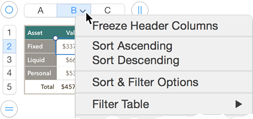
The pop-up menus that you access through the row and column labels are available when a table is active or selected: hover over a label and then click the menu arrow that appears (Figure 12), or Control-click anywhere on the label. I’ll be referring to these as the Row and Column menus from now on.

Although commands for manipulating rows and columns are available in other table menus, these are the safest to use: you’ll always be sure of just which column you might be deleting, or which row is getting three rows inserted above it.

Contextual menus are available from practically anywhere; their commands vary according to whether the table is selected or active, and if there’s a selection within an active table. You can Control-click:

• Table handles: Each of an active table’s four handles—the Table handle, the Column handle, the Row handle, and the Row/Column handle—offers a contextual menu. A selected table has all but the Row/Column handle, and fewer commands available in its remaining menus.
• Inside the table: Control-click anywhere in a selected table, and you get the same menu the Table handle provides. If you Control-click in a cell of an active table, you get a combination of the commands in the Row and Column menus (which makes sense, because a cell belongs to both a row and a column).
• Outside the table: Control-clicking on the background of a sheet always provides a menu with commands for manipulating selected objects; you can, for instance, align them or distribute them evenly across the space (read Manipulating Objects). Commands that are relevant to tables appear in this general contextual menu if a table is selected or active; they are the same as those available from the inside-the-table menu.

Rows and Columns

Whether it’s for looks or a more practical purpose such as moving data into a more logical presentation order, manipulating rows and columns is a basic skill that will serve you well no matter what kind of spreadsheets you create.

Headers and Footers

To make a table’s data understandable, it needs labels, sometimes with subheads, to identify row and column data. And most tables round up aggregate information—even if it’s simply sums—at the bottoms of columns.

A Numbers table can have up to five header rows at the top, five footer rows at the bottom, and five header columns at the left for these purposes. As shown in Figure 13 (ahead a page or so), these are often formatted with fill colors to differentiate them from body rows and columns. But headers and footers are more than just highlighted cells for labels and summaries:

• They are ignored, and rightly so, when a full column or row is referenced in a formula.
• Their content doesn’t show up in autofill suggestions.
• They are not included when you sort your data.
• They can be set to remain visible when you scroll a large table, letting the body rows and columns slide behind them as necessary.
• Their titles can be used in formulas instead of cell references (Rent January instead of B2, for instance), making a formula easier to construct and read.

Add and Delete Headers and Footers

Most, although not all, templates include a header row; some include a column header and/or a footer. It’s easy, however, to create your own headers and footers with one of three basic approaches:

• Format Inspector: This is the most versatile way to add headers and footers, since you can add both in one convenient spot. With the table either active or selected, go to the Table pane of the Inspector and use the pop-up menus in the Headers & Footer section (Figure 13).

• Table menu: The Table menu (on your menu bar) provides many commands regarding header and footers, including submenus from which you can choose the number of header and footer columns/rows that you want. The table can be active or simply selected for these basic commands to be available.
• Pop-up and contextual menus: The Row and Column menus, and a cell’s contextual menu, include header and footer commands when you access them from a spot where headers or footers can be manipulated. So, a menu for an existing header or footer row or column has Add and Delete commands. A menu for a body row, column, or cell that’s next to a header or footer has these commands:
  • Delete: This deletes the adjacent header/footer.
  • Add: This command appears if the table hasn’t reached the header/footer limit.
  • Convert: Choose this to change the row/column to a header/ footer (again, if you haven’t reached the limit).

Freeze Header Rows and Columns

When your table is bigger than your screen (a frequent issue for laptop users), and you scroll to see its far reaches, its headers disappear and you can be left unsure as to what data you’re looking at as it scrolls by.

The solution is to freeze the headers. Choose Table > Freeze Header Rows or Table > Freeze Header Columns (or use a pop-up menu).

If you’d like to see frozen headers in action, open Numbers’ Break-Even Analysis template (in the Business category). Scroll the window contents up and watch the header information disappear. Then, select anything in the table to activate it—even if it’s partially scrolled off the screen—and choose Table > Freeze Header Rows and see what a difference it makes when you scroll the window upward (Figure 14).

Select a Freeze command again to uncheck it and turn off the feature. (I would have preferred a Thaw command.)

Select Rows and Columns

The basic business of selecting rows or columns should be second nature to any Mac user: click on a row label to select the whole row; click on a column label to select the whole column; hold down Shift as you click on cells to add to a selection. But wait, there’s more! I’m referencing only columns in this list to keep your eyes from glazing over at repeated use of the phrase “rows or columns,” but the techniques work for both:

• Select contiguous multiple columns: Drag across their labels in the Column bar.
• Add contiguous columns to a selection: Shift-click another column label to add that column, and all the ones in between; once you click, you can continue dragging to include more columns even if you release Shift. Or, press Shift and an arrow key to add another column.
• Add a non-contiguous column to a selection: Command-click on the column’s label. Add multiple columns by continuing with a drag after the initial Command-click, and the initial gap remains unselected.
• Remove something from the selection: While Command-click is seen as a way to add something to a selection, it’s actually a way to reverse the current selected state. So, Command-click something that’s not selected, and you select it; Command-click a selected item, and it’s deselected.

  For example, if you’ve selected a column because you’re going to format it in italic, or as red text, or as checkboxes, you’ll want to exempt its header cell from that. Command-click the header cell to remove it from the selection before you apply the formatting.

Add and Delete Body Rows and Columns

With cells being the crux of a table and their very existence being dependent upon the intersection of rows and columns, it’s no surprise that there are many ways to add and delete rows and columns. Use the technique that fits your situation—where your pointer is, what your table looks like, what input device you’re using, and so on.

Here are some quick general points:

• When you add rows and columns, the cells inherit text and number formatting from the originating row or column if there’s a selection, or from the last row or column if you add to the edge of a table.
• Alternate-row coloring (applied through the Format Inspector) is automatically adjusted as you add or delete rows.
• There must always be at least one body row and one body column in a table, although there’s no dialog telling you so—nothing at all happens when you try to delete the last of its kind. This is confusing if you have multiple row or column headers that aren’t formatted differently from the body cells—you might not realize you are trying to delete the last body row if you still see five rows in the table.
• General methods for deleting rows and columns, such as those described below, affect only body rows and columns; headers and footers need more direct attention from either the Column and Row menus or the Format Inspector’s cell pane, as described previously in Add and Delete Headers and Footers. If you Option-click to delete a row from the “bottom” of a table, for instance, it’s the last body row that disappears, leaving any footers in place.

Insert or delete at an edge:

• Add at the bottom: Click the Row handle for one row; drag it to add multiple rows.
• Delete from the bottom: Option-click the Row handle to remove one row; Option-drag it to delete multiple rows.
• Add at the right: Click the Column handle to add a single column; drag it to add multiple columns.
• Delete from the right: Option-click the Column handle to delete on column; Option-drag to delete multiple columns.
• Alter the right and bottom simultaneously: Drag the Row/Column handle to add rows and columns; Option-drag it to delete them.

Other ways to insert and delete:

• Row/Column menu: Click a row or column label, and choose a Delete or Add command from its pop-up menu.
• Cell menu: Control-click any cell for a contextual menu that combines the commands from the Row and Column menus (since a cell belongs to both a row and a column).
• Insert command: The Insert > Copied Rows/Columns commands create new rows or columns as necessary to accommodate the copied data, but they have some quirks, as described in Insert Copied Rows and Columns).
• Option-arrow keyboard shortcut: Select a cell, row, or column and then press Option-arrow to add a row or column in the direction of the arrow.

Resize Rows and Columns

There are four convenient approaches to adjusting the size of rows and columns, individually or en masse. I usually refer to only columns here to make the reading easier, but everything also applies to rows.

By dragging:

• Resize one column: Point to the divider line after it in the Column bar (where the letter labels are) to get the resize cursor, and then drag the divider.
• Resize multiple columns: Select them—click and Shift-click, or drag across, the column labels in the Column bar—and then drag either the last or any interior divider. As when resizing the entire table (see Resize a Table), Numbers changes the sizes of the selected columns proportionately, so that if the widest one was twice the size of the others, it will still be twice the size after the resizing.

• Make all selected columns the same width: Option-click the divider after the column whose size you like, and all the selected columns resize to match it. Or, Option-drag the divider after any column to resize it, and the other selected columns resize with it.

By the numbers:

1. Select a single or multiple rows, columns, or cells, and open the Format Inspector’s Table pane.
2. At the bottom of the Table pane, click the Row & Column Size disclosure triangle to expand it if necessary, type or use the arrows to specify the size you want for the row and/or column, and click Fit (Figure 15).

According to cell content:

• Work in the Column bar: Double-click the divider to the right of a column (or at the bottom of a row). If text is not wrapped, a column widens to display all the text; if it’s wrapped (see Text Wrap in Cells), a row expands vertically to display multiple text lines.

  Nothing needs to be selected, as you are specifying the column to adjust by using its divider. If you select multiple columns, double-click on the last divider or any interior one to resize them all.

• Use the Table menu: Select your target column(s) and choose Table > Resize Columns to Fit Content.
• Use the Format Inspector: Select one or more columns and, in the Table pane’s Row & Column Size area, click the Fit button next to Column.

Via even distribution:

• When you want your columns to neatly fill the width of a table, select the table and choose Table > Distribute Columns Evenly (or use one of the table’s menus, described in Pop-up and Contextual Table Menus). This makes all columns the same size.
• If you want only part of a table distributed evenly—say, some columns beneath a mutual, merged-cell header, select the columns first and then use the Distribute command.

Move Rows and Columns

It’s easy to move a row or column to a different spot in the table when you don’t have too far to go. Select it (or them) with a click on its label. Then, click-and-hold the label until the entire row or column seems to lift off the table, and drag it to its new position. (This same procedure is described and illustrated for dragging cells in Five Ways to Create a Table from an Existing Table.)

Keep these points in mind:

• When you’re comfortable with the operation, you’ll notice that you can drag the selection without waiting for the lift-off, although you must briefly release the mouse button (or trackpad) between making the selection and dragging it.
• Dragging a row or column by selecting its label lets you move it to a new spot, but if you select cells in a row or column by dragging across them, and then use the click-and-hold technique to move them, you’ll replace the data where you drop it.
• Formulas update their cell references as necessary when you move rows or columns, just as they do when you copy/paste, autofill cells, or insert new rows, as described in the sidebar slightly earlier, Formula References and Row/Column Adjustments.
• When the new position for the row or column is far away, it’s better to Insert Copied Rows and Columns.

Hide and Show Rows and Columns

There are times when you keep data in a table but don’t need to see it. It’s background information, say, that’s used in a formula but meaningless on its own. Or, you’re going to print (to paper or PDF) and there’s some sensitive data you don’t want to share, such as Social Security numbers in a list of employee information. Alternatively, you might like to see a side-by-side comparison of data that’s separated by intervening rows or columns and want to suppress those interlopers temporarily (Numbers sorely lacks a split-table view!).

In Numbers, you solve these problems with the Hide feature. Hidden rows and columns are out of sight, but not out of mind: if they’re included in a formula, it still uses their content. On the other hand, if you drag across a group of cells and change their format (either cell formats like backgrounds or data formats like the number of decimal places), the formatting isn’t applied to the hidden cells.

For the rest of this section, I’ll refer to only rows, but the same procedures are used for columns.

To hide your data:

• Hide a single row: Choose Hide Row from that row’s Row pop-up menu.
• Hide multiple rows: Select them and choose Hide Selected Rows from the Row pop-up menu for any selected row.

It’s easy to see if rows or columns are hidden when a table is active, since labels will be missing from the Row or Column bar (Figure 16). If you’ve hidden a table’s last row or column, you won’t be able to tell it’s hidden simply by looking at labels; however, if a Row or Column pop-up menu includes the Unhide All command, you’ll know there’s something hiding.

To show your data again:

• Unhide a specific group: Access the Row pop-up menu from a row adjacent to the hidden ones and choose Unhide Rows 6 – 10 (the numbers, of course, are specific to the hidden rows).
• Unhide all rows in the table: Use the Row pop-up menu from any row label and choose Unhide All Rows, or choose Table > Unhide All Rows.

Transpose Rows and Columns

Apple finally added a Transpose command—a standard spreadsheet feature that swaps rows and columns—to Numbers 3.5. To use it on an active or selected table, choose Table > Transpose Rows and Columns. Some formatting might not survive the transposition, as in Figure 17: the bold numbers from the footer row are plain in the transposed table because there’s no such thing as a “footer column,” and the bold formatting came from footer-cell formatting.

Formulas automatically change when necessary on the transposition, but are flagged for your inspection. Click the blue flag to see the original formula; you can compare it to the current, changed formula by looking in the Quick Calculations bar at the bottom of the window (I usually refer to it as the Quick Calc bar), and then clear the warning flag on a per-cell or global basis (Figure 18).