Data Formats

Anyone who uses a spreadsheet is accustomed to typing in text, numbers, or dates and having the spreadsheet automatically recognize what type of data was entered. Ah, would that it were always so simple! In Numbers, there are more than those three categories of data, as well as different ways of displaying identical data types.

Numbers lets you control two kinds of data formatting. There’s the data type: an entry of 3:02 could be a time, or a duration of 3 hours and 2 minutes. And then there’s the data’s look: you enter 2, but it could be displayed as 2.0 or 200%; or, a date could show as December 10, 2001 or 12/10/01 or the European 10 December 2001.

In this chapter, I show you how to use both kinds of data formatting, and how to create Custom Data Formats when Numbers’ built-in options don’t meet your needs.

Standard Data Formats

The Data Format pop-up menu in the Format Inspector’s Cell pane lets you define the type of data in a cell—even overriding a table’s automatic recognition of data types—and control how the data appears no matter how it was entered (Figure 60).

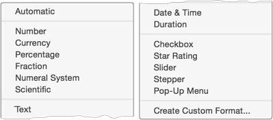
The menu covers five data types, bookended by an all-purpose default and a roll-your-own option:

• Automatic: This is the default. It lets Numbers identify your input so it can right-align numbers, left-align text, automatically format certain things like dates and times, and recognize the equals sign as the beginning of a formula. Based on its identification of cell content, Numbers presents appropriate formatting options in the Cell pane.
• Number formats: These choices control how your numeric entries display. Each has a subset of options so you can tweak things to your satisfaction, such as defining a type of currency or the number of digits in a fraction’s denominator.
• Text: Text has no data-format options; it is what it is.
• Date & Time: As explained a little further on, these are inextricably intertwined, not only metaphysically, but in the way Numbers stores this information.
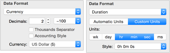
• Duration: This is time from another point of view. Choose from week, day, hour, minute, second, and, yes, millisecond.
• Input controls: These include special items such as Star Ratings and Pop-up Menus.
• Custom formats: These are covered ahead, in Custom Data Formats.

To specify the data type for a cell (or cells), select the cell(s) and then choose a format from the Data Format pop-up menu. From the specifics that appear beneath your choice, define the options for the format, such as how many decimal places to use (Figure 61). You can do this ahead of time, or after the data is entered.

When you type something into a cell that has data formatting applied, you don’t see any formatting until you’ve entered the data by pressing Command-Return or leaving the cell, at which point your formatting magically appears (Figure 62).

When you work in the cell, however, the formatting disappears so you can edit the raw data rather than deal with characters that are inserted as part of the formatting. Double-click the cell to edit it; a single click merely selects the cell, while the second one activates the contents.

Most of the options for the various data types are self-explanatory. And then there are these:

• Automatic data formatting: Cells default to automatic formatting: Numbers decides if you’ve entered a number, text, or date, for instance, and provides options in the Format Inspector’s Cell pane for further formatting. So, type in a number and you’ll get choices regarding decimals and the thousands separator; enter $15.45 and you’ll also get currency-formatting options. But when you keep the Automatic setting in the Cell pane and add formatting, it’s a one-time thing: replace the $15.45 with 12.2 and you’ll have just that unformatted number. To wind up with $12.20, the cell must be specifically formatted for currency.
• Decimals, negative values, and thousands separators: The Number, Currency, and Percentage formats include these options:
  • Decimals: Cells default to showing as many decimal places as you type, but you can set a specific number of places and numbers will be padded out with zeros. The Auto setting in the Decimals section leaves the number as you type it; specify places by typing a number or clicking the up and down arrows next to the field.
  • Thousands separator: If you want commas in your numbers, check this box. If the comma doesn’t display, check The Most Obscure and Annoying Bug Ever, just ahead.
• Dates and times: You can’t really separate these two concepts when it comes to a cell entry; you might use only one side of the coin (a date or a time) but Numbers stores a default for the other. Enter only a time, and Numbers includes the current date; put in a date, and Numbers appends 12:00:00 AM to it behind the scenes. Unless you’ve formatted the cell otherwise, you’ll see only the data you entered—either the time or the date—but if you check the Smart Cell View when the cell is selected, you’ll see the actual contents.

  Define your date and time formats by selecting Date & Time from the Data Format menu. You’ll get separate Date and Time pop-ups that let you show both items in the cell or suppress either one by choosing None from its menu (Figure 63).

Custom Data Formats

While the Format Inspector provides many formatting options for different types of data, it won’t always have the one that you need. Phone numbers and U. S. Social Security numbers aren’t there, for example. But why should you have to type the hyphens for such easily defined patterns? And don’t you want a five-digit zip code whose leading zero won’t drop out? What if you work with a specialized pattern such a membership ID or product number?

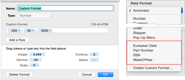
You can handle all these problems and more by creating a custom format through the Format Inspector’s Cell pane, using the Data Format pop-up menu that we’ve covered so far in this chapter as the means for applying pre-defined formats. The menu includes a Create Custom Format command (which opens the Custom Format dialog) and lists your custom formats in their own section (Figure 64).

The basics of creating a custom format are simple:

1. Select one or more cells.
2. Choose Create Custom Format from the Data Format menu in the Format Inspector’s Cell pane.
3. In the dialog that slides out from the window’s title bar, type a name for your format, and choose Number, Date & Time, or Text from the Type pop-up menu.
4. Define your custom format in the Custom Format field. (This, of course, is what the rest of the chapter covers.)
5. Click OK to close the dialog.

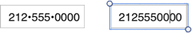
As with standard data formatting applied through the Cell pane, all you have to do is input your data in a custom-formatted cell, and when leave the cell or press Command-Return to deactivate it, the format is applied. Double-click a formatted cell to edit its contents, and you get unformatted data so you don’t have to deal with any formatting characters that are entered automatically (Figure 65).

The other basics you need to know are how to:

• Apply a custom format: Select the cell(s)—before or after you enter data—and choose the format from the Data Format pop-up menu.
• Edit a custom format: Select a cell so that you can access the Format Inspector’s Cell pane; it doesn’t have to be one with the formatting already applied, although Numbers will apply the edited format to the cell. Select the format in the Data Format pop-up menu and then click Edit Custom Format to open the dialog.
• Remove a custom format from a cell: Select the cell and choose Automatic from the Data Format pop-up menu. This removes only the format, leaving any data in its unadorned state.
• Delete a custom format from a document: Select a cell so that you can access the Cell pane, and click the Edit Custom Format button to open the dialog; click Delete Format, and then click Delete again in the confirmation dialog. (File this under There Oughta Be a Better Way.)
• Custom-format availability: If a custom format is in any cell in any table on any sheet of a document, it’s available in the Data Format pop-up menu throughout the document. (Making a Custom-format Library shows you how to use custom formats in other documents without recreating them.)

Custom-format Tokens

Each new version of the Mac OS has made more frequent use of tokens—the little blue lozenges, often with pop-up menus, that stand for some unit of information. They showed up in Finder search fields a long time ago and are used in Apple Mail, too. In Numbers, you can’t build a custom format without them. The tokens in the Custom Format dialog are both crucial and versatile; their versatility means there’s quite a bit to know about them.

To use a token, you drag it from the lower part of the dialog into the Custom Format field (Figure 66).

In the Custom Format field, a selected token appears dark blue; as with selected text, typing replaces a selected token. So, when you want to type something following the token, press the Right arrow to place the blinking insertion point after it, or click anywhere in the format field to deselect the token and place the insertion point.

Most tokens include menus, though that’s not apparent until you’ve dragged one into a format field, at which point the menu arrow appears. So, don’t be fooled by what seems to be a narrow choice of formatting for, say, currency: only the dollar sign shows in the token, but the menu offers two dozen world currencies. You can click directly on the arrow, or Control-click anywhere in the token, to open the menu. (See The Control-click Conundrum for more about tokens and contextual menus.)

A token’s appearance changes in the format field to match the options you choose (Figure 67).

Number Tokens

There’s a plethora of tokens for time and date formats, but their menus are quite straightforward, offering, for instance, a choice of a month format as January, Jan, 1, or 01. Some of the choices for number tokens, however, benefit from some explanation:

• Places for integers or decimals: Change the number of places defined by an Integer or Decimal token with its menu commands (Add Digit, Remove Digit, Number of Digits), or by pressing the Up or Down arrow key when the token is selected (Figure 68).

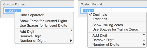
• Commas for thousands: For integers, you can choose to show or hide the thousands separator with the Show/Hide Separator command. If the format is used on cells containing more than three digits, hide the separator if you don’t want a comma. It’s the total number of digits in the final number that counts (no pun intended), not how many are in any one token. So, it’s easy to wind up with a comma in a phone number if you suppress it in only the 4-digit portion of the number.

• Padding with zeros or spaces: For integers, you can choose leading zeros or spaces; for decimals, it’s trailing zeros or spaces.
• Fractions: To display fractions, use the Decimals token and select Fraction from its menu. The menu changes to include a wide array of fractions from which you can choose.

Space Tokens

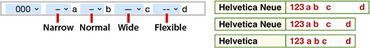
Sometimes you’ll want a space in a custom format—after the parentheses following a phone number’s area code, for instance. You can type it, but it’s hard to see a typed space in the format field. A space token not only makes it clear where a space is, it provides four types of spaces from its menu: Narrow, Normal, Wide, and Flexible. (Not all fonts provide each of the first three or have perceptible differences between them.) A flexible space pushes anything after it to the far end of a cell, no matter how wide the cell, acting as a right tab (Figure 69).

The Data Format Sample

Before we get to actually building some custom formats, let’s take a look at one more area of background information—an ever-so-helpful feature that’s ever-so-confusing until you understand its inner workings: the format sample.

Numbers provides a sample of your format definition in the Custom Format dialog as you design it, and in the Data Format section of the Cell pane afterward. The former can be especially perplexing, because it shows partially defined formatting as you set up your format.

To reduce confusion, select a cell with typical data before you start, since Numbers will use that in the sample instead of a generic default. If the cell you’ve selected:

• Is empty: Numbers uses 1234 as a default number format, 1/5/14 for a default date, or Sample Text for text. If, for instance, you’re creating a format for a ten-digit phone number, the sample 1234 shows this progression as you design the format: 1234-, 1-234, -1-234 (more about that just ahead).
• Has an insufficient number of digits for a number format: You’ll see the same issues as just described, but with your own data (to as many digits as it has) in place of 1234.
• Has “good” sample data: “Good” means it has the expected number of digits, or information that can be interpreted as a date if that’s the format you’re working on. You’ll see the data go through some necessary formatting weirdness, as described next, but when you’ve completed the format definition, it will look fine.

The confusing thing about the sample is that as you design a format, you put elements into the Custom Format field from left to right, while Numbers applies the definition from right to left. As a result, you get peculiar-looking formatting until the last element is in place.

Figure 70 shows the stages of building a simple phone-number format with the correct type of data already in the selected cell. In the first step, the sample is following the pattern as best it can: the hyphen trails the number—so what if there are a lot more digits in the sample? In the second step, there’s a hyphen before and after the last three digits. It isn’t until the last step, with the four-digit token added, that the sample catches up with your reality.

Custom Number Formats

The examples in this section assume you’re already working in the Custom Format dialog: you’ve selected at least one cell, opened the Format Inspector’s Cell pane, and chosen Create Custom Format from the Data Format menu. The first few examples provide more details about working in the dialog; later ones assume you’ve learned those features.

Phone Number

Here’s the step-by-step procedure for the formatting shown in the previous figure:

1. In the Border section of the pane, click the color sample (not the color wheel)—you’ll see a menu arrow appear as soon as your arrow is within the colored area.
2. In the dialog, give the format a name and choose Number from the Type pop-up menu.
3. Format the default integer token in the Custom Format field:
   1. Change it to just three places (so the token has just three pound signs: ###). You can do this with the token selected by pressing Down arrow or you can choose Number of Digits > 3 from the token’s pop-up menu.
   2. From the token’s pop-up menu, choose Hide Separator. (Separators are applied to the total number of digits in a cell, not to the numerals in each token.)
4. Option-drag the token to make a copy, and drop it in the Custom Format field.
5. Type a hyphen between the two tokens, and another one after the second token.
6. Option-drag another token copy, to the far right, and change it to use four places by pressing the Up arrow while it’s still selected.

Your format design looks like this: ###-###-####. If you prefer the parenthetical approach to area codes, type them into the format field with a space after the right parentheses: (#) ###-####.

Social Security Number

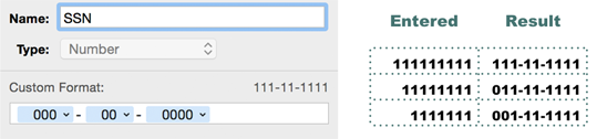
U.S. Social Security numbers are easily formatted: ###-##-####. Here’s how to set that up:

1. In the dialog, name the format and choose Number from the Type menu.
2. Alter the default integer token in the Custom Format field:
   1. Change it to three digits.
   2. Remove the comma by choosing Hide Separator from the token’s pop-up menu.
   3. Here’s the important part: choose Show Zeros for Unused Digits from the token’s pop-up menu so that one or two leading zeros will be preserved if the number starts that way.
3. Type a hyphen after the token.
4. Option-drag the token already in the field to place a copy after the hyphen, and, while it’s still selected from having been dragged, press Down arrow to change it to two digits.
5. Type another hyphen and then Option-drag the second token to after the hyphen; change it to four digits (Figure 71).

Product or Serial Number

Let’s say you’re inputting part numbers that consist of seven digits, used in this pattern: 12-345 [67]. Here’s how to create a custom format for that:

1. Set the first integer token to two places, and hide the separator.
2. Type a hyphen and then Option-drag the token in the field to put a copy after the hyphen; while it’s still selected from having been dragged, press Up arrow to change it to three digits.
3. Type a space and an open bracket [ after the token. (Or, if you’re not comfortable with how a typed space looks in the formatting field, use a space token as I’ve described before.)
4. Option-drag the first token again, and type the closing bracket ].

Note that this does not allow for a leading zero, as you can see in the lower row in Figure 72.

Zip Code

Since I’m assuming you’ve at least read through, the previous examples, we can just zip right through this with a description rather than a step-by-step.

For five-digit U.S. zip codes, use a five-place integer with leading zeros (because the zip codes in my neck of the woods have them). And hide the separator—although this is the last time I’m going to explicitly say that; a comma in your output will be reminder enough from now on.

For nine-digit zip codes, you need two leading-zero tokens separated by a hyphen, so the pattern is simply: 00000-0000. (To see how to handle both kinds of zips in a single format definition, read Alternative Formats with Rules, later in this chapter.)

Custom Date Formats

There’s a wide array of tokens for dates and times, as you can see in Figure 73. Their menus are predictable, providing several formatting choices for each item so you can design formats ranging from 01/05/14 to Sunday, January 5, 2014 and many in between, no matter how a date is entered in the table.

But these formats (and more) are also available in the Cell pane’s Data Format section when you choose Date & Time from the pop-up menu. Of special note in the Custom Format dialog, however, is the second column of tokens for dates, which can effortlessly include date data that is otherwise available only through using Date and Time functions in formulas. So, you can have a date displayed as 04/15/83: Week 16.

Custom Text Formats

Custom text formatting is severely limited in options, and therefore in usefulness. It lets you add text to the text already in a cell, through a single TEXT token that lacks a menu. You can use it to insert labels which, while normally appearing in a column header, could remain with the cell entry when you export data. So, you can “construct” a custom format like the one shown in Figure 74. But since it’s a text format, you can’t append such a label to any number-formatted cell, to get, for instance, SSN: 12-345-6789 or Product: 57-767 [02].

Alternative Formats with Rules

When you create a custom format, you can include alternate formatting to be used if certain conditions—called rules—are met by the data in the formatted cell. So, as in the examples coming up, you can apply formatting to a phone number, but if someone enters a zero, the cell can display N/A. Or, you can format both 5- and 9-digit zip codes in the same cell with one formatting definition.

Set Up a “Not Available” Comment

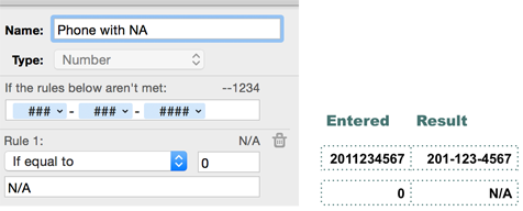
Say you’ve created a custom format for a phone number field that inserts hyphens, as described previously in this chapter. But if a cell is blank in a list of personal information, how could you tell the difference between a cell mistakenly skipped and one for which there was no information available? You’d create a rule inside the custom format definition so that if you enter a zero in the cell it would display N/A:

1. Select a cell and create a custom phone number format for it: ###-###-####.
2. Still in the Custom Format dialog, click Add a Rule, choose If Equal To from the rule’s pop-up menu, and type a zero in the field.
3. In the field beneath the pop-up menu, type what you want to appear if a zero is entered into the field—N/A—and click OK (Figure 75).

Allow for Both 5-digit and 9-digit Zip Codes

Say you need to accommodate two possible inputs—a 5-digit and a 9-digit zip code, for instance. Start by creating a format for a 5-digit zip code. It must allow for the fact that northeastern states have zips that start with a zero (and Puerto Rico a double zero), and if you input numbers with leading zeros, they drop out. So, you use the format 00000 that pads the cell content out to five places.

Next, add a rule that turns more than 5 digits into a format for a ZIP+4 format. Because there’s no way to count the number of digits, you have to think of the zip code as an actual number, and use If greater than 99999 as the condition, and 00000-0000 as the format (Figure 76).

This isn’t stellar, as formatting tricks go, since it’s still not checking for, say, eight digits being mistakenly entered. But custom formatting rules aren’t heavy-duty lifters, and some clever machinations are required when you want to test for more than one condition.

Rule Rules

Now that you know all the basics, here are some of the finer points you should know:

• You can include up to three rules in a format definition.
• Delete a rule by clicking the trash icon in the rule segment.
• Rules are used in order, and when one is met the rest are ignored. So, if your first rule starts with “Less than 100” and the second starts “Less than 10,” the second rule will never be used—because any number less than 10 would also be less than 100, and the rule-processing would end when the first rule is applied.
• You can’t re-order rules. If you want to change the order, you must delete all but the one you want to be first, and then rebuild the others. (Hey, I’m just the messenger!)
• Custom formats live in the spreadsheet where they were created; they are available to every sheet in the document.