Text Functions
Say your friend/brother/boss gives you get an Excel sheet of names and addresses and says: “I need just a list of names (last name followed by a comma and then the first initial); the data came in a little weird and the state abbreviations need to be capitalized; the city, state, and zip code columns need to be combined with a comma (and space) after the city, and a space between the state and zip code, okay? And, oh, can you automatically generate an email address that each person will be assigned—it’s just the last name, the first two letters of the first name, and the company URL?”
Yes, you can do all these things—and easily, since Numbers lets you manipulate text in many ways. In this chapter, after you get acquainted with text terminology, I’ll show you Basic String Manipulations—combining and splitting strings of alphanumeric characters so you can do such things as extract the last name from a cell that holds a full name. Then we’ll look at Other Common Text Tasks such as changing uppercase letters to lowercase, or vice versa, and stripping extraneous spaces out of sloppy data.
Before you reach the end of this chapter, you’ll understand this text-manipulation formula, and why you’d use it:
RIGHT(A2,LEN (A2) - FIND(" ",A2,1)) & ", " & LEFT(A2,FIND(" ",A2,1)-1)
Really. Promise.
Text Terminology
Here’s a turbo lesson in the terms and concepts we use when manipulating text in a spreadsheet:
- A string is any series of characters—letters, numerals, punctuation, and/or symbols. It can be only letters, but doesn’t have to be, and it’s often referred to as a “text string.”
- In formulas, strings appear in quotes: “John” or “Final:” or “.edu”.
- When strings are being compared, everything counts: spaces, punctuation, and case. None of these strings matches any of the others: A well-done steak; A well-done STEAK; A well done steak; a well done steak.
- An empty string is a pair of quotes with nothing inside:
"". It’s often used in a formula to delete unwanted characters (by replacing a character with an empty string—nothing). - You can’t “add” text strings together (how much is “hello” + “there”?). But you can concatenate them by joining them together.
- The ampersand is used to concatenate strings. So, while
2+3equals5, the concatenationhello & thereresults inhellothere. You can type a space on either side of the ampersand to make the formula easier to read, but it’s not necessary; the spaces won’t be used in the calculation. And, as you can see, you need something between the two words, so you’d use a string that’s just a space between quotation marks in the formula:hello&" "&thereresults inhello there.
Basic String Manipulations
Before I provide specific examples, here’s some general guidance for creating your own formulas to handle text strings.
When you need to manipulate text toward a specific outcome, think about the details you need. For instance, for a last name followed by an initial, you need:
last name + a comma + a space + first letter of first name
With a spreadsheet that includes full names, it’s easy to see what the spreadsheet provides (last name and first name) and what you have to add (a comma and a space). Next, you have to think about what function you’d use to extract certain information from what you have (the first letter of the first name). When it comes to figuring that out, the Function Browser can be your best friend (see The Function Browser).
Whether you’re looking at the Function Browser or Apple’s Web site, go to the category that’s most likely to contain what you need (Text, in this case), and scan for a function that sounds like it might serve your purpose. You may be disappointed if you can’t find something that refers to “first,” or some number to find the beginning of a string, but after you see LEFT, RIGHT, and MID in the list, it might occur to you that you need something from the left of the string… and there you have it.
Combine Text Strings
Let’s look at three common text-manipulation procedures that involve combining text information from different cells. You’ll find that using the concatenation operator (&) that glues strings together will quickly become second nature.
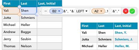
Last Name, First Name
Your table has a column each for first and last name, and your task is to create a column containing lastname, firstname. With the first names in column A and the last names in column B:
- Type an equals sign in
C2(we’re assuming there’s a header inC1) to start the formula. - Click in
B2to put its token in the formula editor. - Type
&", "&(that’s a comma and a space between the quote marks). This begins the concatenation after theB2reference, inserts a comma and a space, and puts in the concatenation operator for the next item you’re entering. - Click in
A2to enter it in the formula, which is nowB2&", "&A2. (OrB2 & ", " & A2, if you prefer a different readability quotient; spaces are ignored unless they’re inside quotes.) - Click Accept
 to enter the formula and see the result.
 - Drag the yellow Autofill handle down in column C to apply the formula to the other names in the list (Figure 108).

Last Name, First Initial
Starting with the same setup as above—first and last names in separate columns—here’s how you construct a last name, first initial column.
There are several text functions that grab specific parts of a text string; in this case, since we want the first letter of a string, we’ll use the LEFT function that lets us specify how many characters we want, starting at the left of the string. The syntax is LEFT(text, number of characters), so that, for example, LEFT("Yonder",2) will resolve to Yo.
Of course, instead of including the text string in the parentheses, you’ll be using a cell reference:
- Start the formula by typing an equals sign in
C2. - Click
B2to reference the last name in the formula. - Type
&","&to add the comma and space after the last name, as well as indicate you’re adding something else to the string. Your formula so far is:B2 &","& - Grab the first letter from the first name in
A2by addingLEFT(A2,1)to this formula. As you start to type LEFT, a token for it appears; press Return to accept the suggested token, and you see the arguments the LEFT function needs: source-string and string-length.Supply them:
- With the source-string token selected, click in
A2(the first-name column), since that’s the source you’re using; the prompt token is replaced by the cell reference. - Select the string-length token with a click or by tabbing to it, and type a 1 to replace it because you want only one letter from the source string.
Your formula is now:
B2 &","& LEFT(A2,1) - With the source-string token selected, click in
- Put a period after the first initial by adding
&"."to the formula (outside the closing parentheses for the LEFT function):B2 &","& LEFT(A2,1) &"." - Press Command-Return to close the formula editor.
- Drag the Autofill handle down from
C2to include your rows of sample data (Figure 109).
Embedded Labels for Output
Back in the Data Formats chapter, I noted that Custom Text Formats are fairly useless in general, and completely so when you need to combine a text format with numeric data for a result such as SSN: 123-45-6789 that you can output in a file that won’t have column labels. It’s easy, however, to make an embedded label for this: concatenate the label and the cell that holds the data. With the Social Security number in B2, the formula is simply: "SSN: "&B2 (note the space included in the label string).
Split Text Strings
Combining text from different cells is relatively simple, but sometimes you have the opposite problem: you need to extract just part of the text that’s in a cell. For instance, you might have a first and last name in a single cell, and want to split them into separate cells so you can sort by last name, or otherwise manipulate them separately.
This gets complicated, because Numbers doesn’t have a function that lets you grab whole words. Instead, you must use the LEFT and RIGHT text functions along with calculations that identify the separating space. If you’re just starting out with Numbers and/or text functions, don’t worry if this is a little confusing at first—it is a little confusing at first, but won’t be for long.
Extract the First and Last Names
Here’s how to build a formula that extracts first and last names from a cell that contains both.
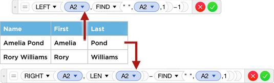
Get the First Name with LEFT
Don’t worry about inputting this formula until you first see how it gets put together, since some of the pieces are a little complicated when you’ve not worked with these concepts before.
The LEFT function gets a specified number of characters starting at the left of a text string. It’s syntax is:
LEFT(this-string, how-many-characters)
Your target string for this example is in A2, where a full name is stored, so this-string is A2. But to get the first name, you need to know how-many-characters it has; to figure that out, you need to first find where the space is between the two names in A2. This is a job for the FIND function:
FIND(this-string, inside-this-string, starting-at-this-spot)
The string you’re looking for is the space between the words; you’re looking inside the text in A2, and you want to start at the first letter, so you use:
FIND(" ",A2,1)
That finds the position of the space, but since you need the number of characters in the first word, which ends just before the space, you need to subtract 1:
FIND(" ",A2,1)-1
That’s the second argument you need for the function:
LEFT(this-string, how-many-characters)
LEFT(A2,FIND(" ",A2,1)−1)
Now that you understand how it’s built, you can put this formula in your example table:
- Click in
B2, the first body cell in the First Name column, and type the equals sign to open the formula editor. - Enter the formula:
- Type
left(until you reach theF, suggestions for other functions will pop up—ignore them), followed by an open parenthesis. - Click in
A2or typeA2to enter its token, and then type a comma. - Type
find, ignoring the suggestions that pop up, and press Return to enter it in the formula. Because FIND is a function that takes arguments, you’ll get tokens for each one it needs, as well as a closing parenthesis. - The search-string token should be selected—it’s darker than the others; if not, click to select it and type
" ". (That’s a space between the quotes.) - Tab to the source-string token to select it, and type
A2or click in that cell. - Tab to the start-pos token and then type
1followed by a closing parenthesis. If you check the Quick Calc bar at this point—it shows the “so-far” results as you create a formula—it seems that you’re finished, because you’ll see the first name there. But what you can’t see is that it’s followed by a space character, which can mess up things later when you try to work with the first name alone. So, make the adjustment I described just before these steps: type-1. Figure 110, a little farther on, shows this formula in a sample table. You can type the final closing parenthesis or let Numbers enter it for you when you close the formula editor. - Click Accept to close the formula editor.
- Type
- Use Autofill to copy the formula down through column B.
Get the Last Name with RIGHT
Extracting the last name is a little more complicated (don’t cringe!) because you can’t slice a string starting from a specific point and going to the end. Nor can you count from the end of a string back to a specific character. But the RIGHT function lets you get characters from the end of a string, going backwards for a specific number of characters:
RIGHT(this-string, this-many-characters-from-the-end)
Once again, this-string is simply the cell that holds the whole name. The second argument needs to use the number of characters in the last name. To find that, we start with the total number of characters in the cell using the LEN (length) function, and subtract everything that’s not the last name: the length of the first name and its trailing space (that part sounds familiar, right?):
LEN(A2) - FIND(" ",A2,1)
The RIGHT function now looks like this (note that the final closing parenthesis belongs to the RIGHT function, not to the FIND function that’s part of the second argument):
RIGHT(A2,LEN(A2)-FIND(" ",A2,1))
This goes in cell C2 of your example table; Autofill it down through column C. Figure 110 shows this and the previous formula at work.
Manipulate the Extracted Names
Once you know how to extract the first and last names from a single cell, you can manipulate them so that, for instance, you can reverse them and use a LastName, FirstName pattern, including the comma. It’s a simple formula:
LastName & ", " & FirstName
But you don’t have to figure the first and last names separately and then use those cells for the formula. Instead, replace LastName and FirstName with the extraction formulas described above to build this whopper—the parts of which you understand completely now, as promised at the beginning of this chapter:
RIGHT(A2,LEN (A2) - FIND(" ",A2,1)) & ", " & LEFT(A2,FIND(" ",A2,1)-1)
Other Common Text Tasks
I’ve been asked many times to manipulate (usually carelessly entered) text in a spreadsheet to standardize it, or make it readable or useable. The most requested fixits, after the text-combining and slicing just described above, fall into the three categories I cover here: letter case, multiple spaces, and the need for email-address generation.
Control Uppercase and Lowercase Letters
The three text functions that let you control upper- and lowercase letters are UPPER, LOWER, and PROPER. The first two give you all capitals or all lowercase letters, and the last capitalizes the first letter of each word in a string and changes the rest to lowercase.
If data comes to you with two-letter state abbreviations either lowercased or with just an initial cap (hey, it happened to me while I was working on this book), use UPPER to capitalize everything:
UPPER("Ma") = MA
Or, if you have a column for “State” in an imported list of addresses, and they’re in all caps (ugh!), you can easily capitalize them properly, whether they’re one or two words, with a single function:
PROPER("OREGON") = Oregon PROPER("NEW JERSEY") = New Jersey
Of course, in usage, the argument for any of these text functions would be a cell reference: PROPER(B2).
As you’ve probably guessed, the LOWER function does just the opposite of the UPPER function; it’s used in the Create an Email Address example a little ahead.
Strip Extraneous Spaces
It boggles my mind that halfway through the second decade of the twenty-first century, so many places still store their data with systems that pad out entries with spaces so that every entry in a category—last name, for instance, or a street name—uses exactly the same number of characters (I’m looking at you, Montclair State University). This is not only so twentieth-century, it’s the first half of the twentieth century. When this data is exported, all those extra spaces come along for the ride. Do a simple calculation like FirstName & " " & LastName and you can get 20 spaces between the names because of FirstName’s trailing spaces—and then there’s LastName’s trailers, too.
To deal with this, use the TRIM function to strip all the spaces from the beginning and end of a string, as well as any extra spaces within a multi-word string so there’s only a single space between the words. For instance (dots indicate spaces):
TRIM("··One·····Two········Three··") results in One·Two·Three
Of course, you’ll have either a cell reference—TRIM(D2)—or another formula as the argument for the TRIM function. So, if you apply the TRIM function to the formula in Last Name, First Name earlier in this chapter—B2 &", " & A2—where B2 holds the last name and A2 the last, it looks like this:
TRIM(B2) & ", " & TRIM(A2)
Notice that TRIM is applied to each data item separately. If you apply it to the original concatenation, like this:
TRIM(B2 & ", " & A2)
you’ll get exactly what you asked for—but not what you wanted. The formula in the parentheses is resolved before TRIM does its work (just as mathematical operations inside parentheses take precedence). If there’s space padding in the original cells, TRIM would be working on:
TRIM(LastName······, FirstName·······)
This results in:
LastName·,·FirstName
You’re stuck with a space before the comma because the comma is an alphanumeric character in the string and is seen as a word; TRIM leaves a space between interior words, so a single space remains in front of the comma.
Create an Email Address
Generating an email address from a last name, the first two letters of a first name, and a company URL is a cinch: you need only two of the text functions already described in this chapter to cobble one together.
Assuming the first names are in column A and the last names are in column B starting in row 2, as described in the Make It note above, your formula would go in C2:
- You’ll want everything in lowercase, so start with the LOWER function:
LOWER() - As LOWER’s argument, concatenate the last name (in
B2) and the two leftmost characters of the first name in column A:B2&LEFT(A2,2). So far, that’s:LOWER(B2&LEFT(A2,2)) - Concatenate the company’s domain name, preceded by the @ symbol, to the string you’ve defined:
&"@example.com". That completes the formula:LOWER(B2&LEFT(A2,2))&"@example.com"
And there’s your email address, as shown in Figure 111.