
2
![]()
Nonlinear Systems and Mathematical Representations
![]()
Dang Van Liet Faculty of Physics, VNU University of Science, Ho Chi Minh City, Vietnam
Le Nguyen Binh
Hua Wei Technologies, European Research Center, Munich, Germany
CONTENTS
2.2 Nonlinear Systems, Phase Spaces, and Dynamical States
2.2.2.1 Fixed Points in One-Dimensional Phase Space
2.2.2.2 Fixed Points in Two-Dimensional Phase Space
2.3.3 Transcritical Bifurcation
2.4.3 Chaotic Nonlinear Circuit
![]()
2.1 Introduction
Nonlinear dynamics have attracted significant research interest and was introduced briefly in Chapter 1. This chapter gives further mathematical details of generic nonlinear dynamic equations and simplified solutions whereby one can generate these nonlinear phenomena in practice.
It is appreciable that nonlinear dynamics can happen due to the nonlinear variations of parameters of physical systems or subsystems in which partial feedback of the outputs of the system reaches an indeterminate state on multistable states at a particular instant. For example in a system consisting of energy storage elements (e.g., inductors and capacitors), the charge and discharge of electrons or currents through or across these elements determine the states of dynamics and stability of the systems, so when both energy storage elements compete for the charges available in the system then chaotic or bistability may occur depending on the rates of storage of energy.
The fundamental rules underlying the shapes and the structures have led to the dynamic study of the nonlinear systems. Especially, modern nonlinear dynamics have focused on analytic solutions of the dynamic equations, and the nonlinearity is determined based on the principles of linear superposition under some approximations such as perturbation techniques. However, fundamental theoretical problems that arise in physics and mathematics as well as in engineering systems can be solved with the assistance of the digital computing techniques.
Solitons and chaos are briefly given, and their potential applications to engineering are given and described in the field of nonlinear optics in the rest of the chapters of this book. In subsequent chapters we will treat soliton and soliton lasers in detail, especially their generation, dynamic behavior, and then transmission over guided optical media.
Surprisingly, simple nonlinear systems are found to have chaotic solutions that remain within a bounded region. In other words, the nonlinearity has been positively considered, and the result has been applied to the analysis and the design in engineering and technology. Thus, nonlinear dynamics in nature have played a key role in physics, mathematics, and engineering, and would be fundamental tools for many branches of future research. This chapter gives a number of mathematical relationships of the principal functions in a nonlinear system and states of the systems in stable or chaotic dynamics bifurcation, as attractors and repellers in such systems. The dynamics of nonlinear systems are also treated in this chapter.
![]()
2.2 Nonlinear Systems, Phase Spaces, and Dynamical States
Nonlinear dynamical systems and chaotic phenomena are used widely in physics and engineering. This section describes some mathematical tools for the analysis of dynamical systems, especially the main pathways to chaos.
2.2.1 Phase Space
Consider a dynamical system represented by a differential equation subject to some initial conditions, for example, a well-known damped oscillation of a mass-spring system, as a mechanical system is governed by the differential equation and initial conditions at t0 [1] given as
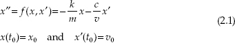
where m is the mass, k is the stiffness of the spring, and c is the damping coefficient. Equation (1.2) is called autonomous because its right-hand side (RHS) does not depend on the time variable. The prime indicates the order of differentiation. In general one can reduce an nth order autonomous ordinary differential equation (ODE) to a system of n first-order DEs then applying the fourth-order Runge–Kutta method to obtain the final solutions of the system.
Let a sinusoidal driving force F exciting on the system, then the DE (2.1) can be rewritten as
![]()
the RHS of (2.2) depends explicitly on time. Equation (2.2) is nonautonomous and can be reduced to a system of (n + 1) first-order DE by replacing the variable t by another dummy variable z. For example, (2.1) can be solved numerically by transforming it into two first-order DEs given by

where x(t) and v(t) represent the displacement and velocity, respectively, and the prime indicates differentiation. In order to examine the behavior of the mass-spring system, the variation of the velocity versus displacement, v(x), is used instead of the time-dependent displacement, x(t). The x-v coordinate system is thus called a phase space, or a two-dimensional (2-D) phase state, of the nonlinear system. Each coordinate represents a variable of the system. The system can thus be represented by an nth-order autonomous differential equation so its phase space has n dimensions. The solutions of the system of (2.3) are subject to a given set of initial conditions under which x(t) and v(t) are determined by a point P in the phase space. When the time t changes then the locus of P follows a curve in the phase space, the phase space trajectory or phase curve. Furthermore, a set of trajectories forms a phase portrait that illustrates the dynamical behavior of the system.
In general, there are three kinds of trajectories in the phase space: fixed points, closed trajectories, and nonclosed trajectories. Figure 2.1 depicts a trajectory of the damped mass-spring system in the phase space operating under the following parameters: m = 1 kg, k = 1.1 Nm–1, c = 0.1 kg–1, x0 = 1, and v0 = 0, t = [0, 20π]. The energy system dissipates its energy in air so the trajectory is a spiral curve toward to the origin O(0,0); the point (0,0) is thus a stable attractor. Figure 2.2 shows the phase portrait of a periodic mass-spring system in the phase space under different initial conditions given by m = 1 kg, k = 1.1 Nm–1, c = 0, x0 = [1, 0.5, 0.3, 0.1], and v0 = 0, t =[0, 20π].

FIGURE 2.1
Trajectory of a damped mass-spring in phase space with an attractor at (0,0).

FIGURE 2.2
Phase portrait of harmonic mass-spring in phase space.
Thus, one can deduce the no-intersecting theorem as follows:
Two distinct state space trajectories can neither intersect (in a finite period of time), nor can a single trajectory cross itself at a phase space at a later time.
2.2.2 Critical Points
The critical point or fixed point in the phase space is the point that corresponds to the equilibrium of the dynamical system. The fixed point can also be the equilibrium point that is an important position, because a trajectory starts at a fixed point and then it stays at this point and the characteristic of the fixed point shows the behavior of trajectories at both its sides.
There are three kinds of fixed points: the attractors, the repellers, and the saddle points. Attractors or nodes or sinks are stable fixed points that attract neighboring trajectories. Repellers or sources are unstable fixed points that repel neighboring trajectories. Saddle points are the semistable fixed points that attract neighboring trajectories on one side and repel those on the other side. Fixed points can be identified without much difficulty. Let’s consider the fixed points in one-dimensional (1-D) phase space which is just a line, we can then extend to those in the 2-D phase space.
2.2.2.1 Fixed Points in One-Dimensional Phase Space
The dynamic equation in 1-D phase space can be written as
![]()
where the prime indicates the differentiation with respect to the position x with respect to time. The fixed points of (2.4) are the locations in the phase space with their value x*′, which must satisfy the condition
![]()
Thus, to find the fixed points, one can solve the equation f(x) = 0, and the solutions x* are the positions of the fixed points. Let’s consider the point xr on the right side and nearby the fixed point x*, if f(xr) > 0 so that x′ > 0, the trajectory starts at xr and moves away from the fixed point; if f(xr) < 0 so that x′ < 0, the trajectory starts at xr moving toward the fixed point, and vice versa for the point xl on the left side and in the neighborhood of the fixed point. If the trajectories at both sides of the fixed point move toward the fixed point, then it can now be called the attractor. On the other hand, if the trajectories at two sides of the fixed point move away from the fixed point then it is termed the repeller. If the trajectory at one side of the fixed point moves toward the fixed point and vice versa for the trajectory at the other side, then the fixed point is classified as the saddle point.
Alternatively, we can use an eigenvalue, λ a characteristic value, to distinguish different types of fixed points that can be obtained by setting
![]()
Then we can approximate this by using the Taylor series to distinguish the kind of fixed point. Let ζ = x – x* and keeping the first two terms of the Taylor series expansion [2,8] in the neighborhood of x*, we have
![]()
On the RHS of this equation the term f(x*) = 0, because x* is defined as the fixed point. So
![]()
The solution of (2.8) is
![]()
ζ is the quantity that measures the distance between a point of the trajectory and the fixed point. The exponential coefficient λ influences the trajectory as follows: (1) If λ < 0, the trajectory moves toward the fixed point exponentially so the fixed point is the attractor; (2) If λ > 0, the trajectory moves away from the fixed point exponentially so the fixed point acts as the repeller; (3) If λ = 0, the fixed point may be the saddle point or the attractor or the repeller. In this case we must compute the second derivative of f(x). If f′′(x) has the same sign at both sides of the fixed point, then that is the saddle point; if f′′(x) > 0 is on the left side of the fixed point and f’(x) < 0 is on the right side of the fixed point, then that is the attractor; otherwise the fixed point is the repeller.
As an example of the attractor and the repeller, consider the equation
![]()
x* = 1 and x* = –1 are the fixed points because f(x*) = 0 ; the eigenvalue at x* = 1 is λ = 2 > 0 so the fixed point at x = 1 is the repeller and its eigenvalue located at x* = –1 with λ = –2 < 0; hence, the fixed point at x = –1 is the attractor (Figure 2.3). The saddle point of the equation x′ = f(x) = x2 is depicted in Figure 2.4 in which the saddle point is located at the origin O(0,0).

FIGURE 2.3
Attractor at (–1,0). Repeller at (1,0).
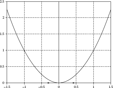
FIGURE 2.4
Saddle point at O(0,0).
2.2.2.2 Fixed Points in Two-Dimensional Phase Space
We can now extend the fixed points in 1-D phase space to 2-D phase space by considering the system of equations
![]()
The phase space is the (x-y) plane, and the behavior of the system is represented by the trajectories in the phase space. Let’s (xc ,yc) be the coordinate of the fixed points satisfying the equations
![]()
The first step is to find the positions of fixed points by solving the system of equations (2.12). Then determine the type of fixed points by finding the characteristic values of the fixed points. The functions f and g depend on the two variables, so the characteristic values depend on their partial derivatives. Similar to the case of 1-D, we are concerned only with the characteristic values in the x and y directions by setting

Thus, we can extend the nature of the eigenvalues in 1-D to classify the types of fixed points in 2-D phase space. We thus consider two distinct cases as follows:
2.2.2.2.1 λ x and λy as Real Numbers
λx < 0 and λy < 0: fixed points are attractors
Considering the equations
![]()
whose solutions can be found as
![]()
We can eliminate the variable t in both x and y to give
![]()
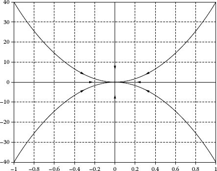
FIGURE 2.5
Attractor in two-dimensional phase space.
The fixed point at the origin O(0,0) and the λx = –1 < 0 and λy = –2 < 0, so O(0,0) is the attractor. We can check this property by inspecting the trajectories. The phase space trajectories are a set of parabolas. For K = 0 the trajectory is the x-axis, when t → 0, x → 0 and y → 0. So all trajectories move toward the origin, and the attractor as indicated in Figure 2.5.
λx > 0 and λy > 0: fixed points are repellers
Considering the equation
![]()
The fixed point is also at the origin O(0,0) and the λx = 1 > 0 and λy = 2 > 0, so O(0,0) is the repeller. The phase space trajectories are the same as the trajectories shown in Figure 2.5, but moving away from the origin, the repeller (Figure 2.6).
λx < 0 and λy > 0. Fixed points as saddle points
In the case that the fixed point on the x-axis is an attractor (λx < 0) and the fixed point on the y-axis is a repller (λy > 0), then the fixed point is the saddle point in the 2-D phase space.
When λx > 0 and λy < 0, we have the opposite situation and the fixed point is now the saddle point.
For example, considering the set of equations
![]()
The variable t can be eliminated in the solution of (2.18), and we have
![]()

FIGURE 2.6
Repeller in two-dimensional phase space.
The phase space trajectories shown in Figure 2.7, are a set of hyperbolae. When K = 0 the trajectory is the x-axis, when t → 0, x → ∞ and y → 0, so the origin is thus the saddle point.
2.2.2.2.2λx and λy as Complex Conjugates
Suppose that
![]()
Then the solutions are
![]()
• If α = 0: the solution x(t) = cosβt and y(t) = sinβt; so the trajectories in the space phase are circles, the fixed point at the origin is called a center (Figure 2.8).
• If α ≠ 0 and β ≠ 0: the fixed point is at the origin that is called a focal point; the solutions are shown by (2.21), and the phase space trajectories oscillate with an angular frequency β. Its amplitudes vary exponentially, so the trajectories move spirally to the origin (attractor) (α < 0) or out of the origin (repeller) (α > 0) (Figure 2.9).
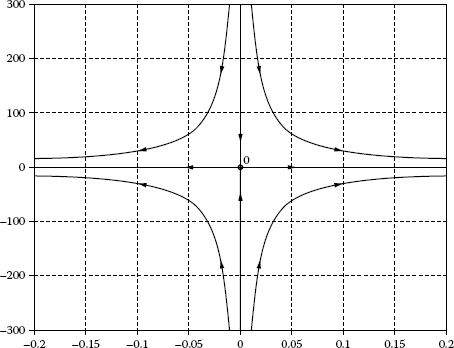
FIGURE 2.7
Saddle point in two-dimensional phase space.

FIGURE 2.8
Center.

FIGURE 2.9
Focus. (a) Attractor. (b) Repeller.
2.2.3 Limit Cycles
In 2-D phase space or higher dimensions, consider a new fixed point that is a limit cycle defined as an isolated closed-loop trajectory in phase space. The neighboring trajectories are opened loops moving spirally in or out of the limit cycle when t → ∞ or t → –∞, respectively. If the neighboring trajectories at both sides move toward the limit cycle, that is a stable limit cycle; on the contrary, the limit cycle is an unstable limit cycle. If the neighboring trajectories at either side of the limit cycle move toward the limit cycle and the others move away, then the limit cycle is a semistable limit cycle. The limit cycle only appears in the nonlinear dynamical system. There are also closed loops in the linear system but they are not isolated, so these closed loops are not limit cycles as shown in Figure 2.2.

FIGURE 2.10
Limit cycle.
Figure 2.10 represents the table limit cycle in phase space (x1 – x2), x1 and x2 are solutions of the equations

where μ is a parameter and the system has a stable limit cycle for μ > 0 like Figure 2.10.
This section can thus be concluded by stating the Poincaré–Bendixson theorem:
• Supposing that there is a bounded region that contains no fixed point, if a trajectory is confined in this region then only either of the following two possible cases can be true: (1) The trajectory is a closed orbit as t → ∞; (2) The trajectory spirals towards a close orbit as t → ∞.
The Poincaré–Bendixson theorem implies that if a trajectory is confined in a closed region that does not contain any fixed point, then at last this trajectory spirals to a closed orbit. For a higher-order dimensional system (n ≥ 3) the trajectories may wander forever in a bounded region. The trajectories are attracted to a complex geometrical object, the strange attractor. This is the characteristic of a chaotic phenomenon. The chaotic trajectories cannot appear in 2-D phase spaces.
![]()
2.3 Bifurcation
As described above, a dynamical system can be represented by a differential equation. If the equation depends on only one or more parameters then the fixed points of the system can be altered accordingly. These qualitative variations of the dynamical system are termed bifurcation. In this section, we briefly present the bifurcation in 1-D and 2-D phase spaces. Further, we restrict our discussion to the most common types: the pitchfork, the saddle-node, the transcritical, and the Hopf bifurcations [1,2,8].
2.3.1 Pitchfork Bifurcation
This bifurcation occurs most commonly in symmetrical systems. As an example of pitchfork bifurcation consider the equation
![]()
where μ is a real parameter. This equation is invariant when x is replaced by –x. To study the bifurcation of this system, we have to find the fixed points and their characteristics.
• The positions of fixed points are determined by
![]()
so there are three fixed points at ![]()
• The characteristics of the fixed points are determined by
![]()

FIGURE 2.11
Pitchfork bifurcation diagram. Solid lines: stable state equilibrium. Dashed line: unstable state equilibrium.
When λ < 0, the fixed point is stable, the attractor. However, if λ > 0, then the fixed point is unstable, the repeller.
• If μ < 0, there is only one fixed point at the origin (x1 = 0) and it is stable (λ = μ < 0).
• If μ > 0, there are three cases: (1) The fixed point at x1 = 0 is unstable (λ = μ > 0); (2) the fixed point at is stable (λ = –2μ < 0); and (3) the fixed point at is stable (λ = –2μ < 0).
We can thus solve the system of equations (2.24) and (2.25) to obtain x = 0 and μ = 0. The origin (x = 0, μ = 0) is the bifurcation point.
The diagram of the pitchfork bifurcation is shown in Figure 2.11, the solid lines indicate the positions of stable fixed points, and the dashed line indicates the positions of unstable fixed points. This case is the supercritical pitchfork bifurcation because the bifurcation branches are stable. The other case is called the subcritical pitchfork bifurcation when the bifurcation branches are unstable.
2.3.2 Saddle-Node Bifurcation
This bifurcation is the basic mechanism. In this case the fixed points are created or destroyed as one or more parameters of the system change. As an example of the saddle-node bifurcation, consider
![]()
with μ a parameter that can take positive, negative, or zero values. The fixed point and its characteristics are determined by
![]()
and
![]()
• If μ < 0 the system has two fixed points, the stable fixed point A at ![]() (l < 0) and the unstable fixed point B at
(l < 0) and the unstable fixed point B at ![]() (l > 0) (Figure 2.12a).
(l > 0) (Figure 2.12a).
• If μ → 0, the parabola moves up and two fixed points A and B move together. When μ = 0 two fixed points A and B add together to be a half-stable fixed point at the origin O (x = 0) (Figure 2.12b).
• If μ > 0 the system does not have any fixed point (Figure 2.12c).

FIGURE 2.12
Saddle-node bifurcation process in the phase space: (a) m < 0; (b) m = 0; (c) m > 0.

FIGURE 2.13
Saddle-node bifurcation diagram.
The system of equations (2.27) and (2.28) can be solved to give solutions x = 0 and μ = 0, so the bifurcation point can be located at the origin (x = 0, μ = 0).
We can now depict the curves of x′ = 0 in the space (μ, x); the curves (C) of function μ = –x2 represent equilibrium positions of x on μ (Figure 2.13). Figure 2.13 shows the saddle-node bifurcation diagram. This is the common way to illustrate the saddle-node bifurcation, which can also be called a fold bifurcation or a turning-point bifurcation because the point of x = 0 and μ = 0 is a turning point.
2.3.3 Transcritical Bifurcation
In this bifurcation the fixed point of the system always exists but its characteristics change as one or more parameters change. As an example of the transcritical bifurcation consider the equation
![]()
where μ is a parameter that can take values of positive, negative, or zero. The fixed point and its characteristics can be determined by
![]()
and
![]()

FIGURE 2.14
Transcritical bifurcation process in the phase space: (a) μ < 0; (b) μ = 0; (c) μ > 0.
• If μ < 0 the system has two fixed points, the stable fixed point at x1 = 0 (λ < 0) and the unstable fixed point ) (λ > 0) (Figure 2.14a).
• If μ = 0 the system has a half-stable fixed point at the origin O (x = 0) (λ = 0) (Figure 2.14b).
• If μ > 0 then the system has solutions of two fixed points, the unstable fixed point at x1 = 0 (λ > 0) and stable fixed point (λ < 0) (Figure 2.14c).
Combining three cases shown in Figures 2.14a, 2.14b, and 2.14c, we see that the fixed point located at the origin (x = 0) always exists but its stability changes as m varies. So this is the case of transcritical bifurcation.
The solution of system of equations (2.30) and (2.31) gives the bifurcation point at the origin (x = 0 and μ = 0). Thus we also use the space (μ, x) to represent the transcritical bifurcation diagram as shown in Figure 2.15.
2.3.4 Hopf Bifurcation
Hopf bifurcation occurs when a limit cycle is taken from a fixed point as one or more parameters of the system vary, and it takes place only in the phase space of higher-order dimensions (≥2). In this section we present the Hopf bifurcation in 2-D phase space. As an illustration of the Hopf bifurcation, consider the system of equations

FIGURE 2.15
Transcritical bifurcation diagram.

where μ is a real parameter. This system is simpler when transformed into polar coordinates (r,θ) by setting x1 = rcosθ and x2 = rsinθ with (2.32), we thus have
![]()
Equation (2.33) shows that there are two fixed points at r1 = 0, because the solution can be eliminated by setting r > 0 and the eigenvalues λ = μ ± i.
If μ < 0 there is only a stable fixed point at the origin that is the focus; the trajectories spiral the origin (Figure 2.16a). If μ = 0, the origin, that is a center, is also a stable fixed point, the trajectories also spiral the origin slowly (Figure 2.16b). If μ > 0 the fixed point at the origin (r = 0) is unstable and the fixed point at ![]() is stable, the trajectories become a stable limit cycle (Figure 2.16c).
is stable, the trajectories become a stable limit cycle (Figure 2.16c).

FIGURE 2.16
The birth of the limit cycle of Hopf bifurcation: (a) m = –0.1 < 0; (b) m = 0; (c) m = 0.3 > 0.
We can see that when μ < 0 the origin is stable and when μ > 0 the origin is unstable and appears to be a stable limit cycle with ![]() So the Hopf bifurcation occurs at μ = 0, and it is called the supercritical Hopf bifurcation because the limit cycle is stable. The diagram of the Hopf bifurcation is depicted in Figure 2.17. We also have the subcritical Hopf bifurcation when the limit cycle is unstable. Hopf bifurcation is also called the oscillatory bifurcation.
So the Hopf bifurcation occurs at μ = 0, and it is called the supercritical Hopf bifurcation because the limit cycle is stable. The diagram of the Hopf bifurcation is depicted in Figure 2.17. We also have the subcritical Hopf bifurcation when the limit cycle is unstable. Hopf bifurcation is also called the oscillatory bifurcation.
Bifurcations play important roles, because in some dynamical systems, when the control parameter increases for a long time, the bifurcations may appear several times. This is then followed by the wandering unpredictably of the system’s trajectories in the phase space. This is the chaotic phenomenon.
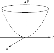
FIGURE 2.17
Hopf bifurcation diagram.
![]()
2.4 Chaos
2.4.1 Definition
There is no exact definition of chaos, but the commonly accepted definition [8] is: “Chaos is aperiodic long term behavior in a deterministic system which is strongly dependent on its initial conditions.”
Under this definition, a chaotic phenomenon appears only when the system evolves for a long time, during which times there are no intersections of different aperiodic trajectories produced by the system represented by a DE associated with some certain deterministic initial conditions. The system is sensitive to its initial conditions meaning that there are two neighboring trajectories beginning at the distance d0, and the time-dependent distance is given by d(t) = d0eλt (λ > 0), with λ is known as the Lyapunov exponent, so two neighboring trajectories can move away with respect to each other exponentially.
E. N. Lorenz (1963) conducted the first experiment on chaos [3]. His model is a simplified model of the fundamental Navier-Stokes equation of the dynamics of fluids given by

where p is the Prandtl number, r is the Rayleigh number, and b > 0 is an unknown parameter. He solved (2.34) numerically and realized that the system was sensitive to its initial conditions, and the system trajectories neither settle at any point nor repeat again but always follow a spiral, and no intersection of trajectories would occur. He then termed this image the Lorenz attractor (Figure 2.18) (p = 10, r = 28, b = 8/3). This is a chaotic phenomenon. Currently this is called the attractor of a chaotic system, which is a strange attractor or chaotic attractor or fractal attractor as shown in Figure 2.18.

FIGURE 2.18
Variation of z with respect to x. Strange attractor.
2.4.2 Routes to Chaos
The trajectories of nonlinear systems may move from a regular to a chaotic route pattern when a control parameter changes. These are the transitional routes to chaos. There are several types of routes to chaos [4]. In this section we review only some main routes to chaos.

FIGURE 2.19
(a) Chua’s circuit. (b) The driving-point characteristic of the nonlinear resistor NR in Chua’s circuit. (Chua’s equations are as given in M. P. Kennedy (1994), “ABC (Adventures in Bifurcations and Chaos): A Program for Studying Chaos,” Journal of the Franklin Institute, 331B(6), 631–658.)
2.4.2.1 Period Doubling
As described in the above sections the limit cycle was born from the bifurcation that relates to a fixed point. As a control parameter changes, the limit cycle would be unstable and onset to periodic-doubling limit cycles. The control parameter continues to change so that the period doubling becomes unstable and a period-four cycle starts to appear. The process will continue to infinite-period cycle, and then trajectories follow the chaotic behavior.
As an illustration of period doubling, consider Chua’s circuit, a simple nonlinear circuit that leads to chaotic behavior:
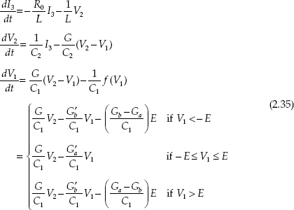
in which the conductance of the elements is given as G = 1/R, G′a = G + Ga and G′b = G + Gb.
Using the Kennedy’s values [5], L = 18 mH, R0 = 12.5 Ω, C2 = 100 nF, Ga = –757.576 μS, Gb = –409.09 μS, E = 1 V, C1 = 10 nF. By changing the control parameter G we have the phase portraits in Figure 2.20. Figure 2.20a shows a single-period limit cycle, G = 530 μS. Figure 2.20b shows a period-doubling limit cycle with G = 537 μS, and Figure 2.20c is a quadrupling period limit cycle, G = 539 μS. Figure 2.20d depicts a spiral Chua’s chaotic attractor with G = 541 μS. Figure 2.20 thus shows the sequence of dynamics leading to the doubling period and thence the route to chaos.

FIGURE 2.20
Phase portraits. (a) T period solution, G = 530 mS. (b) 2T period solution; G = 537 mS; (c) 4T period solution; G = 539 mS; and (d) chaotic solution, G = 541 mS.
2.4.2.2 Quasi-periodicity
The motion of a nonlinear dynamic system that associates with two frequencies is called the quasi-periodic motion, and it appears when the ratio of two frequencies is not a ratio of integers. So the motion does not repeat itself exactly but is not chaotic.
The quasi-periodic route to chaos is connected to the Hopf bifurcation. In Section 2.2 we considered the Hopf bifurcation that associates with the onset and the start of the limit cycle, a periodic motion, from a fixed point. In some nonlinear dynamical systems, the first and then the second Hopf bifurcation appears when the control parameter changes. If the ratio of frequencies of the second and the first motion is not rational, then the motion of the system is quasi-periodic. If the control parameter continues to change, then a chaotic motion would appear. This route is called the Rouelle–Takens route.
Figure 2.21 represented a quasi-periodic signal that is the voltage of the second capacitor in Chua’s circuit using an inductor gyrator (see Figure 2.23).

FIGURE 2.21
Quasi-periodic signal.
2.4.2.3 Intermittency
The intermittency is the motion that is nearly periodic with irregular bursts appearing from time to time. The phenomenon appears pseudo-randomly and not purely random because the system is represented by a deterministic equation. There can be two approaches to the intermittency: (a) the motion of system changes between the periodic motion and the chaotic motion and (b) the motion of system changes between the periodic motion and the quasi-periodic motion.
In some nonlinear dynamical systems, the control parameters of the system change further and the irregular bursts appear frequently so that the intermittency behaviors become chaotic behaviors. We will observe the intermittency motion in the next section.
2.4.3 Chaotic Nonlinear Circuit
The Chua’s circuit using the inductor gyrator was investigated by Bharathwaj Muthuswamy et al. [7]. The schematic of the inductor gyrator is given in Figure 2.22, and its impedance is given:
![]()
In 1992, K. Murali and M. Lakshamanan [6] examined the effect of the external periodic excitation on Chua’s circuit. We can now consider a Chua’s circuit with external driving sinusoidal excitation, and this circuit used the inductor gyrator instead of an inductor because the inductor is cumbersome for the integrated circuit to be used in an experiment.

FIGURE 2.22
Circuit of inductor gyrator. (From B. Muthuswamy, T. Blain, and K. Sundqvist (2009), “A Synthetic Inductor Implementation of Chua’s Circuit,” Technical Report No. UCB/EECS-2009-20. Access date: June 2011, http://www.eecs.berkeley.edu/Pubs/TechRpts/2009/EECS-2009-20.html. With permission.)
Figure 2.23 shows the schematic of Chua’s circuit using an inductor gyrator with a sinusoidal excitation. The state equations for Chua’s circuit (See Figure 2.19a) are given:

FIGURE 2.23
Chua’s circuit using inductor gyrator and sinusoidal excitation.

where is a piecewise-linear function given by
![]()
Ga, Gb, and E were shown in Figure 2.19b, and f is the frequency of the external sinusoidal excitable source connected to the induction gyrator.
From the schematics of Figure 2.22 and Figure 2.23 we can design an electronic circuit as shown in Figure 2.24. Figure 2.24a,b,c shows the circuit diagram, the realization of the electronic Chua’s circuit using the inductor gyrator, and the experimental measurement setup, respectively. A signal generator excites a sinusoidal voltage to the circuit, and an oscilloscope is used to capture the dynamic nonlinear behavior of the output point of the circuit versus the input excitation source.
We fixed the values of all elements of Chua’s circuit and consider F and f as the control parameters. If the amplitude F and frequency f are varied by changing the external excitable voltage, the dynamical behavior of Chua’s circuit can be observed and examined.
2.4.3.1 Simulation Results
Using equations (2.27) and (2.38), setting the values RL = 10 Ω, Rg = 100 kΩ, C = 16 nF, C1 = 9.8 nF, C2 = 100 nF, Ga = –0.756 mS, Gb = –0.409 mS, E = 1.08 V, R = 1770 Ω. The amplitude of excitation voltage F = 275 mV and its frequency can be employed as the control parameters, and we can observe the following cases:
• Case 1: Vf = 0, this is the motion of the Chua’s circuit using the inductor gyrator, and we get the typical Chua’s attractors as in Figure 2.25.
• Case 2: F = 275 mV, f varies from 25 Hz to 500 Hz, we also get the typical double scroll of Chua’s attractor and look like a combination of two single attractors. The motion behaviors are more complex (Figure 2.26).
• Case 3: F = 275 mV and f varies from 516 Hz to 1545 Hz, we get a cascade of period adding when decreasing the frequency of sinusoidal excitation (Figure 2.27).
• Case 4: Keeping F = 275 mV and f increasing from 1800 Hz, we can realize some different cases. At f = 1929 Hz, the dynamical system is represented by a point-attractor (Figure 2.28a) and after that the system will be chaotic. At f = 1967 Hz we get two single scroll attractors and it also exits limit cycles (Figure 2.28b). At f = 3333 Hz, two single scroll attractors extend their sizes and meet together to be a double scroll attractor with limit cycles at the outside. (Figure 2.28c) At f = 4287 Hz, there is a typical double scroll attractor (Figure 2.28d).

FIGURE 2.24
Chua’s circuit experiment: (a) principle diagram with the details of elements, (b) electronic Chua’s circuit using inductor gyrator, and (c) experimental system.

FIGURE 2.25
Typical Chua’s attractor: (a) (v1-v2) phase space, (b) (v1-v3) phase space, (c) (v3-v2) phase space. (In this figure v3 = iL.)
2.4.3.2 Experimental Results
We can set R = 1720 Ω so that the circuit behaves chaotically by itself without any sinusoidal excitation or self-excitation in order to study the dynamical behavior of the circuit when it is excited by an external sinusoidal force.
• Bifurcation diagram

FIGURE 2.26
Attractors at F = 275 mV, (a) f = 27 Hz, (b) f = 275 Hz, (c) f = 400 Hz.
• We change the value of driving source amplitude F from 25 mV to 400 mV with the step of 25 mV; at every amplitude we decrease the driving source frequency f from 9 KHz to 0 KHz with step varying from 5 Hz to 20 Hz. We monitored (v1 − v2) (v1 and v2 are voltages dropped across the capacitors C1 and C2, respectively), the phase space on the oscilloscope depicts the bifurcation diagram in the (F-f) plane. Figure 2.29 is the bifurcation diagram with f changes from 200 Hz to 4000 Hz; the numbers denote the periods (adding periods) of attractors, and the shaded regions denote chaos.
• In the region of the driving source frequencies greater than 4000 Hz, the bifurcation only changes from single-scroll to double-scroll attractors and vice versa as illustrated in Figure 2.30.
• Period doubling

FIGURE 2.27
Period adding at F = 275 mV. (a) Period 1, f = 1545 Hz. (b) Period 2, f = 1017 Hz. (c) Period 3, f = 798 Hz. (d) Period 4, f = 624 Hz.
• A cascade of period doubling bifurcations appears in the middle frequencies from 3000 Hz to 4000 Hz (Figure 2.29). At F = 275 mV, typically one period appears at driving source frequency f = 3582 Hz (Figure 2.31a). We then decrease f to 3333 Hz to obtain a double-scroll attractor (Figure 2.31b). At f = 3040 Hz a Hopf bifurcation appears with an outer limit cycle (Figure 2.31c). However we do not observe any period doubling, period quadrupling, or period octupling trajectories in this cascade structure. This may be due to the fact that the state of the system has reached the limit of the bandwidth of the oscilloscope.
• Period adding

FIGURE 2.28
Attractors at F = 275 mV. (a) f = 1929 Hz. (b) f =1967 Hz. (c) f = 3333 Hz. (d) f = 4287 Hz.

FIGURE 2.29
Bifurcation diagram in (F- f) plane. The numbers are the periods, and the shaded regions are chaos.

FIGURE 2.30
Relation of single-scroll attractors and double-scroll attractors in (v1-v2) phase space. (a) f = 8.29 KHz. (b) f = 6.8 KHz. (c) f = 6 KHz. (d) f = 4.4 KHz (horizontal axis: 1 V/div and vertical axis: 0.5 V/div).

FIGURE 2.31
Period doubling at F = 275 mV. (b) Two-scroll attractor, f = 3333 Hz. (a) and (b) h axis: 1 V/div and v. axis: 0.5 V/div. (c) Limit cycle, f = 3040 Hz, h. axis: 5 V/div, v. axis: 2 V/div.

FIGURE 2.32
A cascade of period doubling in (v1-v2) phase space at F = 275 mV. (a) through (i) from Period 1 to Period 10. (Horizontal axis: 1 V/div and vertical axis: 0.5 V/div.)
• In Figure 2.29, the region of excitable frequencies of less than 1200 Hz is called the region of periodic windows. In this region chaotic behaviors and the period doubling appear sequentially. Figure 2.32 represents a cascade of period doubling at the excitable amplitude F = 275 mV, and the order of period increases when the excitable frequency decreases.
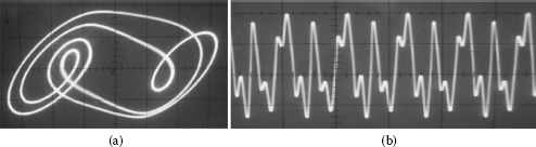
FIGURE 2.33
Quasi-periodicity at F = 100 mV and f = 2954 Hz. (a) Trajectories in (v1-v2) phase space. (Horizontal axis: 1 V/div and vertical axis: 0.5 V/div.) (b) v1 voltage.
• Quasi-periodicity
• With quasi-periodicity, the system has two different frequencies that associate together so the motion of the system is called quasi-periodic motion and it repeats itself inexactly. In our experiment, the quasi-periodic behaviors at the excitable frequencies are less than 3000 Hz according to the excitable amplitude appropriately. Figure 2.33 depicts the trajectories in the phase space (v1-v2) and its signal v1. When the excitable frequency is changed slowly, the quasi-periodic motion alters to chaotic motion.
• Intermittency
• In this experiment, the intermittent behaviors appear in the excitable region with frequency greater than 1000 Hz. Figure 2.34 depicts the trajectories in the phase space (v1 − v2) and its voltage v1 to illustrate the intermittent behavior. We realized that the periodic oscillations are interrupted by the intermittent bursts. Figure 2.35 depicts the intermittent behavior near the boundary crisis region.
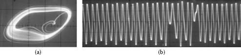
FIGURE 2.34
Intermittency at F = 275 mV and f = 1731 Hz. (a) Trajectories in (v1-v2) phase space. (Horizontal axis: 1 V/div and vertical axis: 0.5 V/div.) (b) v1 voltage with intermittent bursts.

FIGURE 2.35
Intermittency near the boundary crisis region at F = 400 mV and f = 1475 Hz. (a) Trajectories in (v1-v2) phase space. (Horizontal axis: 1 V/div and vertical axis: 0.5 V/div.) (b) v1 voltage with intermittent bursts strongly.
![]()
2.5 Concluding Remarks
In this chapter we presented briefly the main principles of a nonlinear dynamical system. The descriptions of fixed points, bifurcation, and chaos are explained. Further main routes to chaotic states of nonlinear systems are obtained and derived from the mathematical point of view and then experimental demonstration. In the last section Chua’s nonlinear circuit is illustrated experimentally using an inductor gyrator in association with appropriate resistors and capacitors excited with the external sinusoidal source so that the charging and discharging can happen simultaneously so that chaotic behavior can be observed in both simulation and experiment. This chaotic behavior and nonlinear dynamical evolution will be illustrated in the remaining chapters of this book in several fiber optic lasers of different feedback structures in the optical domain.
Bifurcation and chaotic dynamics of fiber laser systems will be illustrated in Chapters 7 and 8 in which the envelopes of the lightwaves behave in nonlinear motions illustrated in the mathematical representations given in the above sections.
The basic mathematical representations of other nonlinear optical systems described by other chapters would be briefly described in their contents.
![]()
References
1. N. V. Dao, T. K. Chi, and N. Dung, An Introduction to Nonlinear Dynamics and Chaos, Vietnam National University Publishing House (in Vietnamese), Hanoi, 2005.
2. R. C. Hilborn, Chaos and Nonlinear Dynamics: An Introduction for Scientists and Engineers, Oxford University Press, New York, 1994.
3. E. N. Lorenz, “Deterministic Nonperiodic Flow,” Journal of the Atmospheric Sciences, 20(2), 1963.
4. T. Kapitaniak, Chaos for Engineers: Theory, Applications, and Control, 2nd edition, Springer, Berlin., 1998
5. M. P. Kennedy, “ABC (Adventures in Bifurcations and Chaos): A Program for Studying Chaos,” J. Franklin Inst., 331B(6), 631–658, 1994.
6. K. Murali and M. Lakshmanan, “Effect of Sinusoidal Excitation on the Chua’s Circuit,” IEEE Trans. Circuits and Systems–I: Fundam. Theory and Appl., 39(4), 264–270, 112, April, 1992.
7. B. Muthuswamy, T. Blain, and K. Sundqvist, “A Synthetic Inductor Implementation of Chua’s Circuit,” Technical Report No. UCB/EECS-2009-20, 2009. Access date: June 2011, http://www.eecs.berkeley.edu/Pubs/TechRpts/2009/EECS-2009-20.html
8. S. H. Strogatz, Nonlinear Dynamics and Chaos: With Applications to Physics, Biology, Chemistry, and Engineering, Westview Press, Boulder, CO, 2000.