Chapter Ten

 

 

Anti-windup for Euler-Lagrange Plants

10.1 FULLY ACTUATED EULER-LAGRANGE PLANTS

This chapter focuses on a specific case study where the model recovery anti-windup (MRAW) construction described in Section6.3 is applied to a class of nonlinear plants consisting of all fully actuated Euler-Lagrange systems. In particular, for all such plants, an anti-windup construction is given here that, provided that some feasibility conditions are satisfied, is able to recover global asymptotic stability of the closed loop with saturation as long as the unconstrained controller guarantees global asymptotic stability and local exponential stability of the unconstrained closed loop.

This case study can be understood as an example of how far the techniques illustrated in this book can reach beyond the linear and arguably simpler situations addressed in the other chapters. Clearly, nonlinear plants require more specific and tailored solutions; however, the model recovery architecture and a carefully designed feedback-stabilizing signal v can guarantee successful anti-windup in most reasonable nonlinear application studies.

Fully actuated Euler-Lagrange systems correspond to mechanical systems characterized by some generalized position variables q ∈ ⁿ, a so-called Raleigh dissipation function (q, ) R(q, ) = 1/2 ^TR(q), and a so-called Lagrangian function (q, ) L(q, ), defined as L(q, ) = T(q, ) – V(q), where T(q, ) is the kinetic energy of the system and V(q) is its potential energy. As usual in classical mechanics, the kinetic energy can be written as T(q, ) = 1/2 ^TB(q), where q B(q), called generalized inertia matrix, is a differentiable function, symmetric positive definite and globally bounded away from zero and from infinity. In other words, there exist positive numbers λ_M and λ_m such that λ_mI ≤ B(q) ≤ λ_MI for all q ∈ ⁿ (where I denotes the identity). For the remaining parameters, it suffices that the potential energy q V(q) and the dissipation matrix q R(q) be differentiable, but weaker conditions would also be compatible with the solution given here.

The dynamics of a fully actuated Euler-Lagrange system can be written as

(10.1)

where u denotes the generalized external forces applied to the system. Fully actuated means that the number of independent inputs u in the previous equation is equal to the number of generalized position variables n.

A special class of the fully actuated Euler-Lagrange systems described above is given by the following equations describing the dynamics of fully actuated robotic manipulators:

(10.2)

where C(q, ) represents the generalized centrifugal and Coriolis terms, h(q) is the vector of gravitational forces and the function R(q) represents the friction forces. The relation between equations (10.1) and (10.2) is easily derived as

Since the matrix B(q) is nonsingular for all values of its argument q, then equations (10.1) and (10.2) can be rewritten as

(10.3)

where F₁(q, q_d, u) := q_d and F₂(q, q_d, u) is uniquely defined by the Lagrangian function and the Raleigh dissipation function. For example, when using the description (10.2),

In the rest of the chapter, the two notations (10.1) and (10.3) will be used interchangeably.

Given the Euler-Lagrange system (10.1), assume that the following unconstrained controller

(10.4)

(where x_c ∈ ^nc is the controller state, u_c ∈ ²ⁿ is the controller input and r ∈ ⁿ is the external reference input) has been designed in such way that for any selection of r within a prescribed set of admissible references, the unconstrained feedback interconnection

(10.5)

guarantees global asymptotic stability and local exponential stability of a point (x^*,x^*_c) where x^* = (q^*,q^*) = (r,0).

Then the anti-windup problem addressed here is that of recovering the possible stability and performance loss due to input saturation, experienced in the following saturated closed-loop interconnection between the plant (10.1) and the controller (10.4):

(10.6)

where sat (·) is the magnitude saturation function with symmetric saturation levels ₁,…,_n

10.2 ANTI-WINDUP CONSTRUCTION AND SELECTION OF THE STABILIZER V

Model recovery anti-windup for the saturated closed loop described in the previous section can be performed by generalizing the compensation scheme for linear plants as outlined in Section 6.3 on page 161. In particular, for the problem analyzed here, where f characterizes the plant with input saturation and F characterizes the plant without input saturation, equation (6.8) characterizing the anti-windup filter dynamics becomes

(10.7)

where the anti-windup state x_aw = (q_aw, q_aw) has the same dimension as the state of the plant. The dynamics (10.7) is used in a model recovery anti-windup framework to enforce modifications on the unconstrained controller, as follows:

(10.8)

where v is the stabilizing signal to be designed in such a way that the anti-windup dynamics (10.7) is driven to zero and model recovery is obtained, as illustrated in Chapter 6.

Similar to the anti-windup solutions for linear plants given in Chapters 7 and 8, also in this case, regardless of the nonlinearity of the plant, the selection of v is a key aspect of successful anti-windup augmentation. The solution proposed next is guaranteed to induce closed-loop global asymptotic stability and performance recovery whenever the following condition holds:

(10.9)

The meaning of equation (10.9) is quite intuitive when looking at the special case of robotic manipulators in equation (10.2). Indeed, since in that case, denotes the gravitational forces, equation (10.9) requires that there be enough input authority to induce any desired steady-state position q = r on the robot. The construction for v given here can also be carried out when condition (10.9) is not satisfied. However, in that case there is only a local asymptotic stability guarantee on the resulting closed-loop system.

Whenever condition (10.9) is satisfied, the selection of v can be done as follows:

(10.10)

where K_q and K_g are diagonal positive definite constant matrices and K_qd(.,.) is a diagonal positive definite matrix function which is constant in a sufficiently small neighborhood of the origin and bounded away from zero,¹ and such that the function (q_aw, _aw)K_qd(q_aw, _aw)_aw is locally Lipschitz in all its arguments. Moreover, K_g is chosen in such a way that

(10.11)

where K_gi are the diagonal entries of K_g. Note that as long as condition (10.9) holds, there always exists a small enough matrix K_g that satisfies constraints (10.11)). If, however, constraints (10.9) do not hold, then it is possible to select K_g without satisfying (10.11) and the resulting anti-windup compensation will not guarantee global properties.

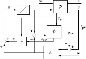
Figure 10.1 Model recovery anti-windup for Euler-Lagrange systems.

The anti-windup construction outlined above is represented in Figure 10.1. Note that as compared to the typical model recovery anti-windup scheme discussed in Chapter 6, full state measurement is required here from the plant because the anti-windup dynamics depends both on x_aw and on x. The anti-windup construction is summarized step by step in the following algorithms, where two possible solutions are given. The first one corresponds to a constant selection of K_qd(·,·) and is therefore a simpler scheme with lower performance. The second one corresponds to to a nonlinear selection of K_qd(·,·) and leads to improved performance.

Algorithm 24 (MRAW for Euler-Lagrange systems with linear injection)

Step 1. Choose a diagonal positive definite n × n matrix K_g whose diagonal entries K_gi, i = 1,…, n satisfy the constraints (10.11). Typically, select the entries K_gi as the maximum allowable within the constraints (10.11). If the compatibility condition (10-9) does not hold, then select any positive definite diagonal K_g and only local asymptotic stability will be guaranteed.

Step 2. Augment the saturated closed-loop system with the anti-windup compensator (10.7) interconnected via (10.8) and where v is given in (10.10) with the constant selection K_qd (q_aw, q_aw) = K₀, where K₀ and K_q are still to be defined.

Step 3. Select the positive diagonal entries K_qi and K_0i, i = 1,…, n of K_q and K_o, respectively, following a standard PD tuning technique at each joint.

The next algorithm provides a further improved action by selecting K_qd(.,.) as a nonlinear function. The idea behind this selection is that it coincides with the linear one proposed in the previous algorithm as long as the saturation function multiplying K_g in equation (10.10) is not active. However, when that saturation becomes active, the nonlinear selection of K_qd(.,.) allows to suitably scale down the right term at the last line of (10.10) as much as the left term at that last line is scaled down by the saturation effect. It will be clear from the simulations reported in the example cases studied next that the nonlinear selection leads to highly improved closed-loop performance.

Algorithm 25 (MRAW for Euler-Lagrange systems with nonlinear injection)

Step 1. Choose a diagonal positive definite n × n matrix K_g whose diagonal entries K_gi, i = 1,…, n satisfy the constraints (10.11). Typically, select the entries K_gi as the maximum allowable within the constraints (10.11). If the compatibility condition (10-9) does not hold, then select any positive definite diagonal Kg, and only local asymptotic stability will be guaranteed.

Step 2. select K_qd(q_e, _e) = γ E(q_e, _e)K₀, where the parameter K₀ is a diagonal positive definite matrix and the diagonal matrix function γE(.,.) = diag {γE1 (.,.),…, γEn(.,.)} has diagonal entries corresponding to

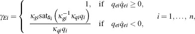
where sat _i(·) is the symmetric scalar saturation function with limits _i.

Step 3. Augment the saturated closed-loop system with the anti-windup compensator (10.7) interconnected via (10.8) and where v is given in (10.10) with the function K_qd(·,·) defined at the previous step, and where K₀ and K_q are still to be deined.

Step 4. Select the positive diagonal entries K_qi and K_0i, i = 1,…, n of K_q and K0, respectively, following a standard PD tuning technique at each joint.

10.3 SIMULATION EXAMPLES

In this section some simulation examples are reported to demonstrate the proposed anti-windup construction. The first two examples will be useful to appreciate the proposed construction in simple linear case studies. The next example shows the performance of the proposed construction in a simple nonlinear robot arm. Finally, the construction is applied to models of two industrial robots, the PUMA robot and the SCARA robot.

Prior to starting to describe the example studies, the following section clarifies some specific unconstrained controller selections carried out in the examples. Note that no constraint is given on the controller selection as long as it stabilizes the nonlinear Euler-Lagrange system without saturation, therefore the two approaches described next could be replaced by any alternative stabilizing selection.

10.3.1 Selection of the unconstrained controller

Since only unconstrained closed-loop stability is required by the unconstrained controller, this could be selected among a large variety of control laws for Euler-Lagrange systems that populate a vast literature on robotics research distributed over the last three decades. It is noteworthy that, due to the model recovery architecture of the anti-windup solution, the anti-windup compensator dynamics and the selection of the parameters in the function γ(·,·) illustrated in Algorithms 24 and 25 are only related to the plant dynamics and are independent of the unconstrained controller.

Among the many possible selections of the unconstrained controller, two most typical approaches are reported next and will be used in the following simulation examples. Detailed descriptions of these and other unconstrained control laws can be found in any classical robot control textbook.

1. Proportional-integral-derivative regulator with a nonlinear gravity compensation (otherwise called PID+h(q)). This controller is typically used for set-point regulation purposes and can be written in the form (10.4) as follows:

(10.12)

where r is the reference input corresponding to the desired joint position, K_p, K_i and K_d are suitable positive deinite diagonal matrices representing the proportional, integral and derivative gains, and V(q) is the potential energy of the system. When using the notation in (10.2), equation (10.12) can be written as

2. Feedback linearization with extra PID action (otherwise called “computed torque” + PID). This control technique employs feedback linearization to linearize the unconstrained Euler-Lagrange system. Then any arbitrary lineardecoupled behavior is imposed on the resulting unconstrained closed loop by means of an extra decentralized PID compensation action, so that decoupled behavior is obtained, in addition to arbitrary linear performance. This controller is typically used for trajectory tracking purposes and the corresponding controller equations in the form (10.4) are given by

(10.13)

where K_p, K_d, K_i are suitable diagonal matrices, B(q) is the generalized inertia matrix, and r and denote a desired reference profile and its derivative with respect to time, respectively. Note that due to the special structure of the Lagrangian function and of the kinetic energy, the second equation in (10.12) is independent of because the term B(q) cancels out with the corresponding term resulting from the first term of the right-hand side. In particular, when using the notation in (10.2), equation (10.12) is equivalent to the following simplified form:

where r and represent the trajectory to be tracked.

10.3.2 Academic examples

The three examples addressed here are simple control systems aimed at illustrating step by step the construction in Algorithm 25.

Example 10.3.1 (Double integrator) Consider a double integrator, which could represent a unit mass moving on a horizontal rail without any friction. Assume that the control input has an input saturation level M = 0.25. Select the unconstrained controller as a stabilizing PID controller with gains (k_p, k_i, k_d) = (8,4,4). Since the Euler-Lagrange equations for this simple system are linear (they actually are = u), then the resulting anti-windup compensator equation is extremely simplified and, based on (10.7), (10.8), corresponds to

with . It should be also noted that in this case, due to the linearity of the plant dynamics, the anti-windup compensator does not require any plant state measurement because the two terms at the right-hand side of equation (10.7) reduce to F (x_aw, u — y_c).

Since the potential energy for this example is constant, the selection of γ(·,·) in (10.10) only depends on x_aw = (q_aw, _aw). Based on the construction in Algorithm 25, the signal v in (10.10) is then selected as

Regarding the selection of the scalar parameters K_g, K_q, and K₀, according to step 1 of the algorithm, K_g is selected as K_g = 0.99, which is the maximum value satisfying equation (10.11). Then the two other gains are selected similarly to the tuning procedure for PD gains with the goal of obtaining a desirable response recovery. This leads to the selections K_q = 80 and K₀ = 100.

Figure 10.2 The double integrator in Example 10.3.1. Responses to a unit reference.

The closed-loop responses to a unit step reference of the unconstrained, saturated, and anti-windup closed loops are represented in Figure 10.2. The unconstrained response (dashed) rapidly converges to the desired steady-state exhibiting a slight overshoot. The saturated response (dotted) diverges in an oscillatory way and the anti-windup response (solid) shows a fast and graceful recovery of the unconstrained response.

Example 10.3.2 (Planar positioning system) Consider a positioning system consisting of a two-link robot, with two linear joints. The model is quite simple: the robot is not subject to the gravitational force, the generalized inertia matrix is linear and decoupled, and so is the matrix containing the friction terms. A schematic diagram of the planar positioning system is reported in Figure 10.3.

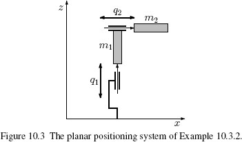
The system model is expressed by the following equations:

(10.14)

where M_i is the total mass of each link (including the actuator's mass), ρ_i is the friction coefficient of the ith link, and u_i is the ith actuator's force. The values of parameters are reported in Table 10.1, where _i is the saturation level of each actuator.

Table 10.1 Parameters of the planar positioning system of Example 10.3.2.

The unconstrained control system is a “computed torque” controller, which is able to induce global exponential stability when saturation does not occur. The performance of the unconstrained controller is obtained choosing suitable values for the diagonal matrices K_p, K_d, K_i. The equations of the unconstrained controller are:

where represents the controller input, so that the unconstrained interconnection corresponds to the saturated interconnection (without anti-windup) corresponds to , and the anti-windup interconnection corresponds to, is the anti-windup compensator's state. The proportional, integral, and derivative gains of the unconstrained controller have been selected as follows: K_p = diag(360,360), K_d = diag(30,30), K_i = diag(8,8).

The anti-windup construction is carried out following Algorithm 25. In particular, the anti-windup compensator dynamics (10.7) become:

where u = [u₁,u₂]^T is the force plant input that, according to equation (10.8), is selected as:

where sat(·) is the saturation function having symmetric saturation limits ₁ = ₂ = 40 and k_qd1 (.,.) and k_qd2 (.,.) are the diagonal elements of the matrix function K_qd(.,.) selected at step 2 of the algorithm.

As for the selection of the diagonal matrix gains K_g, K_q, and K₀, since there is no gravity effect on this model, it is possible to select K_g arbitrarily close to the identity, e.g., K_g = diag(0.99,0.99), which satisfies constraint (10.11). The remaining matrix gains K_q and K₀ should be selected with the goal of improving the performance of the anti-windup law during the transient response. For each entry i = 1,2 on the diagonal of K_q and K₀, the proportional term K_qi is selected so as to guarantee a fast enough convergence of the related component of q_aw to zero, and the derivative term K_0i is selected so as to enforce suitable damping on the terminal part of the trajectory, thus avoiding undesirable oscillations of the anti-windup closed-loop response. Following this approach, the parameters are easily tuned as K₀ = diag(650,250), K_q = diag(2600,1600).

Figure 10.4 Output responses for the planar positioning system in Example 10.3.2.

Figure 10.5 Input responses for the planar positioning system in Example 10.3.2.

The anti-windup construction is tested by simulation by selecting the reference signal as the following step input:

(10.15)

and initializing both the plant and the controller states at zero. The corresponding simulations are reported in Figures 10.4 and 10.5. In Figure 10.4, the bold curves represent the unconstrained output responses. The output responses of the anti-windup closed-loop system (thin solid) reach the reference positions in less than one second, eliminating the undesired oscillations exhibited by the saturated closed-loop system without anti-windup (dotted). Figure 10.5 represents the plant input responses for the same three closed-loop systems. Note that the anti-windup action exploits the full actuator's power available to allow for the fast output responses of Figures 10.4. This fact becomes evident when noticing that the plant input signals become saturated both during the acceleration and during the deceleration phases.

Example 10.3.3 (Two-link planar robot with rotational joints) Consider the planar two-link robot arm represented in Figure 10.6, displaced on a vertical plane so that the gravitational vector is oriented as shown in the figure. Differing from the previous example, the robot dynamics is nonlinear and not decoupled, and the gravitational acceleration affects both links. The aim of this example is to show the quasi-decoupled performance of the anti-windup closed-loop system in the presence of input saturation and the easy selection of the anti-windup parameters.

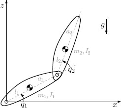
Figure 10.6 The two-link planar robot with rotational joints in Example 10.3.3.

According to the notation used in equation (10.2), the generalized inertia matrix B(q), the matrix C(q, ) related to the centrifugal and Coriolis terms and the gravitational vector h(q) are given next. For simplicity, the friction forces are set to zero. The generalized inertia matrix B(q) corresponds to:

with

where q = [q₁, q₂] contains the two joint variables, (M₁, M₂) are the total masses of the two links (including the actuators’ masses), (a₁, a₂) represent the link lengths, (i₁, i₂) represent the distances of the center of mass of each link from the preceding joint, and (I₁,I₂) represent the rotational inertias at the two joints. The matrix C(q,) can be written as follows:

and the gravitational forces vector corresponds to

where g is the gravitational acceleration value. The physical parameters of the robot have been selected as shown in Table 10.2, where (₁,₂) represent the saturation levels for the torques exerted at the two joints.

Table 10.2 Parameters of the two-link planar robot in Example 10.3.3.

As in the previous example, the unconstrained controller is selected as a computed torque controller, which induces linear and decoupled closed-loop behavior before saturation is activated. The corresponding equations are:

where represents the controller input interconnected to the closed loop in the same way as in the previous example. The proportional, integral, and derivative gains of the unconstrained controller have been selected as K_p = diag(240,255), K_d = diag(45,50), and K_i = diag(4,4).

According to equation (10.7), the anti-windup compensator's dynamics can be written as:

where y_c is the unconstrained controller output and v is selected according to Algorithm 25 as

where σ₁(.) and σ₂(.) denote the two input saturation functions and k_qd1 (.,.) and k_qd2 (.,.) are the diagonal elements of the matrix function K_qd (.,.) defined at step 2 of Algorithm 25.

The diagonal elements of the matrix K_g have been chosen to satisfy the constraint (10.11) as K_g = diag(0.29,0.64). The diagonal elements of the matrices K_q, K₀ have been selected once again following the approach at step 4 of Algorithm 25. The resulting matrices are K₀ = diag(150,400) and K_q = diag(400,400).

Figure 10.7 Output responses for the two-link planar robot in Example 10.3.3.

For the simulation tests, the reference signal has been selected as a step input, assuming the following values:

(10.16)

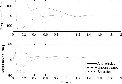
Figure 10.8 Input responses for the two-link planar robot in Example 10.3.3.

and both the plant and the controller states have been initialized at zero.

The corresponding simulations are reported in Figures 10.7 and 10.8. As usual, the dashed curves represent the unconstrained responses, the dotted curves represent the saturated responses (without anti-windup), and the solid curves represent the anti-windup responses. Observe that the undesired undershoot presented by the saturated response is completely eliminated by the anti-windup action. Moreover, the anti-windup compensation is able to almost fully preserve the linear performance at the second joint. This is not the case in the first joint response, which exhibits an inevitable response delay due to the input limitation.

From the input responses reported in Figure 10.8, it appears that the anti-windup compensator makes large use of the available input effort. Nevertheless, the input signal doesn't reach saturation other than for a short time interval during the first 200 milliseconds. This suggests that increasing the anti-windup gains Kq and K0 may lead to a faster response. Additional simulations, which aren't reported here, confirm that increasing the anti-windup gains to the values K₀ = diag(600,400) and K_q = diag(4000,400) allows to reduce the recovery transient on the first joint from approximately 1. 5 seconds to 1 second (the response on the second joint remains the same).

10.3.3 SCARA robot

10.3.3.1 Model description and anti-windup design

The SCARA robot (Selective Compliance Assembly Robot Arm) is a four-link robot, with four joints, all of them having vertical axes. The first two links of the robot reproduce the behavior of a planar two-link robot on a horizontal plane (hence, they are not subjected to gravity due to structural constraints); the third link is connected to a linear joint which is used to impose the tilt of the end effector on the working plane; and the last joint is a rotational joint that allows the roll movement of the end effector for manufacturing purposes.

Table 10.3 Parameters of the SCARA robot.

Based on the physical parameters of the robot, which are selected as shown in Table 10.3, a quantitative Euler-Lagrange model of the form (10.2) can be derived for the SCARA robot. For simplicity of notation, assume that the center of gravity of each link is located at its middle point. Table 10.3 reports, for each link the length l_i of the link, the total mass M_i of the link (including the actuators’ masses), the rotational inertia I_i of the link, and the saturation level _i of each actuator. The viscous friction, corresponding to the matrix R(q) in equation (10.2), is assumed to be zero for the purpose of illustration. In all the following simulations, the performance of the anti-windup closed-loop system has been tested in the case where uncertainties affect the model of the robot. To this aim, the actual masses of the robot have been chosen to be 20% more than the nominal ones listed in Table 10.3. Moreover, to represent a payload held by the end effector, the mass of the last link is 0.5 kg larger than that of the model.

For the SCARA robot, after verifying that this system with the saturation levels in Table 10.3 satisfies equation (10–9), it is possible to apply Algorithm 25 and to design an anti-windup compensator inducing guaranteed global asymptotic stability. In particular, the selection of the parameters of the stabilizing function γ(·,·) is carried out as in steps 1 and 4 of the algorithm, thus resulting in

10.3.3.2 Setpoint regulation

The anti-windup closed-loop system is first tested on a setpoint regulation problem. To this aim, the unconstrained controller is chosen to be the PID + h(q) controller in (10.12). The setpoint simulations carried out correspond to the following selection of the reference input:

(10.17)

In particular, the PID gains of the unconstrained controller are selected as

(10.18)

Moreover, to provide a fair comparison among the different responses, following standard control techniques for industrial robots, the reference signal is smoothened by a cubic interpolation joining the initial zero configuration to the desired vector goal. If the time interval to join the initial configuration to the desired position is large enough, then the corresponding control inputs are regular functions that don't reach the saturation limits, thereby avoiding undesired oscillations and possible stability loss. For the setpoint (10.17), this time interval is chosen as 1.8 seconds, which is the minimum allowable before the occurrence of saturation at the first joint.

On the other hand, the closed-loop system with anti-windup augmentation can be driven directly by the step reference input (10.17) because the anti-windup action ensures closed-loop stability in any operating condition and achieves unconstrained response recovery regardless of the occurrence of saturation. Note that this feature simplifies the regulation task because it doesn't require the computation of the smoothened reference profile, in addition to guaranteeing an improved closed-loop performance, as shown by the following simulations.

The responses of the PID + h(q) controller with smoothened reference and of the PID + h(q) controller with anti-windup action are reported in Figures 10.9 and 10.10. The initial conditions of the plant, controller, and anti-windup blocks are always set to zero. In both figures, the solid curves represent the anti-windup responses while the dotted curves represent the saturated responses with smoothened reference input. As a term of comparison, the dashed curves reproduce the unconstrained responses in the absence of saturation. These responses represent the ideal performance of the system with this unconstrained controller. Indeed, the (virtual) absence of saturation allows driving the closed loop directly with the step input and observing a fast and smooth convergence to the desired steady state. This type of response is, of course, only ideal and not reproducible on the saturated plant. Nevertheless, it represents a good comparison means for evaluating the performance of the two other responses in terms of their mismatch with that unconstrained one.

From the solid and dotted curves in Figures 10.9 and 10.10 it appears that the closed loop with anti-windup compensation, in addition to not requiring the computation of the smoothened reference, guarantees a faster convergence to the desired setpoint. This property is a consequence of the fact that the anti-windup action does not fear the occurrence of saturation but makes use of saturated signals to suitably drive the plant output to the desired values (see Figure 10.10). On the other hand, the reference smoothing strategy deliberately avoids the occurrence of saturation for the closed loop without anti-windup, so that undesired oscillatory behavior may not occur, thereby leading to a slower closed-loop response. Note that the reference smoothing solution is crucial for this particular application because when the saturated closed loop reaches saturation even for a very small amount, persistent and very large oscillations are triggered on the closed loop, thus leading to disastrous effects. This has been preliminarily illustrated in Section 1.2.7 on page 16 and is not reported here due to the choice of using a more industrially relevant smoothed reference solution.

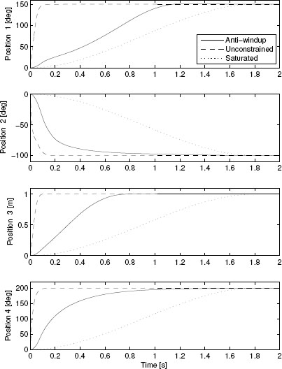
Figure 10.9 Output responses to the reference (10.17) of various closed loops for the SCARA robot.

10.3.3.3 Trajectory tracking

In a second set of simulations, the anti-windup scheme is tested on a trajectory tracking task where the control input demanded by the unconstrained controller persistently transits inside and outside the saturation limits. The trajectory that the robot is supposed to track corresponds to a circle on the horizontal plane centered at (x₀,y₀) = (0.15m, 0.15m) and having radius 0.1 m. The circle should be tracked by the end effector at an angular speed of 0.9π rad/s. To guarantee perfect tracking on the unconstrained plant, the unconstrained controller is selected as the computed torque + PID controller (10.13), which is driven by a suitable reference r(t) and its time derivative (t). For simplicity of exposition, the PID gains of the controller have been chosen as in (10.18). Indeed, experience indicates that the performance of the closed loop is almost independent of the selection of the PID gains. What is

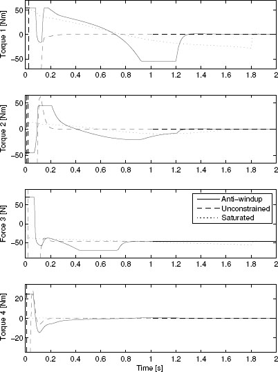
Figure 10.10 Input responses to the reference (10.17) of various closed loops for the SCARA robot.

mostly responsible for bad saturated responses is the feedback linearizing action of the computed torque controller.

Figures 10.11 and 10.12 show the three responses of the anti-windup (solid), unconstrained (dashed), and saturated closed loop. The saturated closed loop is equipped with a simple “integrator shut-off” strategy, which is a well known heuristic used to combat actuator saturation in classical control systems.

Only the responses of the first two joints are reported because they are the most interesting ones. The three closed-loop systems are all initialized at the position (q₁,q₂,q₃,q₄) = (92 deg, -109.23 deg,0 m,0 deg) along the circular trajectory (with zero initial velocity), so that it is possible to appreciate the steady-state behavior, rather than the transient responses, which are well characterized by the previous set of simulations.

Due to the high coupling between the two links and the aggressive control action arising from the feedback linearizing components of the controller, the saturated response is unable to preserve stability and exhibits persistent oscillations of increasing amplitude. This is apparent from the top and mid-lower plots of Figure 10.11, where the dotted curves depart from the two other ones at time t = 1.5. After this time, the saturated response is most of the time out of range in the plots of Figure 10.11. Accordingly, in Figure 10.12 the dotted trajectory leaves the circular trajectory in unpredictable directions. (For graphical purposes, the dotted responses have been limited to the time t ∈ [0,2] seconds on this last figure, as this is sufficient to show its unacceptable behavior that persists in future times.) On the other hand, the anti-windup closed-loop system performs well, due to the fact that the anti-windup compensator is able to rapidly drive the plant state back toward the unconstrained response. This is particularly evident in the two top plots of Figure 10.11, where, from the solid curves, it appears that the control signal is kept in

Figure 10.11 Input and output responses of the first two joints in the reference tracking simulation for the SCARA robot.

Figure 10.12 End effector trajectory on the horizontal plane in the reference tracking simulation for the SCARA robot.

saturation (lower plot) so as to drive the first joint angle toward the unconstrained angular response (top plot). Based on this recovery property, the trajectory is corrected by the anti-windup action at each period immediately after saturation and, as shown in Figure 10.12, the effector position response only slightly deviates from the ideal circular reference path.

10.3.4 PUMA robot

10.3.4.1 Model description and anti-windup design

The PUMA robot (Programmable Universal Machine for Assembly) is a six degrees of freedom robot with six rotational joints. By way of the six degrees of freedom, the end-effector position and orientation can be arbitrarily configured in the three-dimensional space. In particular, the first joint axis is vertical and the second and third joint axes are parallel and horizontal. The remaining joint axes intersect at one point: the center of the spherical wrist. The presence of the spherical wrist allows assigning in a decoupled way the orientation and the position of the end effector.

The physical parameters of the robot have been selected as shown in Tables 10.4 and 10.5 based on the information available from the literature. Based on these physical parameters, a dynamical model of the robot can be written in the form (10.2). For each link, Table 10.4 reports the total mass M_i, including the actuators’ masses (the mass of link 1 is irrelevant because the center of gravity of the first link

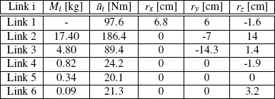
Table 10.4 Parameters of the PUMA robot.

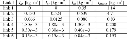
Table 10.5 Diagonal terms of the rotational inertias and motor inertias.

never moves), the maximum motor torque _i, and the coordinates r_x, r_y, r_z of the center of gravity of each link, referred to the corresponding link reference frame according to the Denavit-Hartenberg standard notation. For each link, Table 10.5 also reports the rotational inertias I_xx, I_yy, I_zz and the motor and drive inertia I_m, expressed in terms of the Denavit-Hartenberg reference frame, translated onto the link center of gravity. The viscous friction, corresponding to the matrix R(q) in equation (10.2), is assumed to be zero for the purpose of illustration. To better illustrate the anti-windup effectiveness, assume that the actuator saturation level for the PUMA robot is one-third of the actual values reported in Table 10.4. Under these circumstances, controlling the robot becomes a harder task to accomplish, while on the other hand lighter and cheaper actuators may be mounted on the system. To illustrate robustness, in the following simulations the masses of the robot links have been increased by 20% with respect to their nominal values (listed in Table 10.4). Moreover, to represent a payload held by the end effector, the mass of the last link is 0.5 kg larger than that of the model.

This PUMA robot complies with the requirement in equation (10.9), even when the saturation levels correspond to one-third of the values in Table 10.4. Then it is possible to achieve guaranteed global asymptotic stability following the construction in Algorithm 25. According to this construction, the anti-windup parameters are selected as:

10.3.4.2 Setpoint regulation

The anti-windup performance has been tested on the PUMA robot by simulating the response to a setpoint regulation task. The unconstrained controller has been chosen to be a PID + h(q) controller because it has been noted that alternative choices did not lead to aggressive enough responses and would have appeared too slow as compared to the anti-windup ones. On the other hand, the PID + h(q) controller with a suitably smoothened reference signal via cubic interpolation proved to be the best controller selection among the typical control strategies for set-point regulation of industrial robots. To induce a nice unconstrained response on the six robot joints in the small signal case (i.e., in the absence of saturation), the PID gains of the unconstrained controller have been selected as follows:

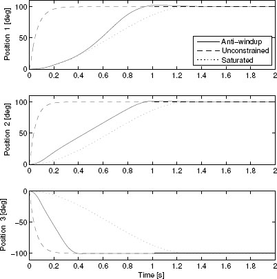
Figure 10.13 Output responses to the reference (10.19) of various closed loops for the PUMA robot.

Figure 10.14 Input responses to the reference (10.19) of various closed loops for the PUMA robot.

To suitably appreciate the effects of the anti-windup action on the PUMA dynamics, a very large setpoint value has been selected as:

(10.19)

and the following closed loops have been simulated comparatively:

1. The unconstrained closed-loop response obtained by interconnecting the controller directly to the Euler-Lagrange system without any input saturation.

2. The saturated closed-loop system corresponding to the interconnection of the unconstrained controller to the plant with saturation while the reference input is smoothed in a similar way as in Section 10.3.3. To obtain improved performance with the saturated closed loop, the PID gains have also been shrunk to the values and based on these values the reference has been smoothed via cubic interpolation to join the initial and final joint configurations in 1.3 seconds.

3. The anti-windup closed-loop system corresponding to the interconnection of the unconstrained controller to the plant with saturation and without any reference smoothing. As in the SCARA example addressed in the previous section, due to the ability of the anti-windup compensator to handle the occurrence of saturation, the anti-windup closed-loop system is driven directly by the bare step reference. The anti-windup action will automatically take care of achieving a closed-loop response, which gracefully converges to the desired steady state regardless of the occurrence of saturation.

The simulation results are reported in Figures 10.13 and 10.14 where the position outputs and the torque inputs of the first three joints are reported. The responses on the remaining three joints are not reported because they are very comparable to the response of the third joint. Indeed, on the last joints the robot dynamics is almost negligible due to the low masses and inertias of the links and it is possible to enforce an almost decoupled behavior on the closed-loop system, which is not of much interest here.

From Figure 10.14 it is evident that the saturated response makes large use of the actuators within the saturated region. This is one of the features that allows achieving the high-performance response of Figure 10.13, where the solid curves converge to the desired set point at a faster speed than the saturated response without anti-windup. It is stressed once again that the high-performance response induced by the anti-windup action corresponds to a control scheme which does not require the extra computational burden arising from determining a cubic interpolant for the reference signal. Also in this case, as in the previous section, the saturated response without reference smoothing is not shown in the figures. That response leads to extremely large and undesirable overshoots and undershoots in the first three joints and is a quite unreasonable solution from an implementation viewpoint.

10.4 NOTES AND REFERENCES

The model recovery anti-windup solution illustrated in this chapter was first outlined in [MR4] and then better illustrated and extended in [MR19], which also contains the SCARA simulations reported here. The remaining examples treated here are taken from [MR18]. As in [MR18] and [MR19], the parameters of the SCARA robot have been taken from [G7], while the parameters of the PUMA robot have been taken from [G2] and [G4]. An explanation of the “integrator shut-off” heuristic used in the simulation of Figure 10.12 can be found, e.g., in [SUR5].

---

¹A diagonal positive definite matrix function K_qd(·,·) is bounded away from zero if there exists a small enough positive scalar k_d such that K_qd(·,·) ≥ k_dI for all values of its arguments.