
Chapter Seven
Linear MRAW Synthesis
7.1 INTRODUCTION
Figure 7.1 represents the model recovery anti-windup (MRAW) scheme introduced in Chapter 6. In that scheme, the upper block P represents the plant, the lower block K represents the unconstrained controller and the intermediate block Pcap, which corresponds to a model of the plant, contains the dynamical states of the anti-windup augmentation. This structure permits recovering information about the unconstrained response, so that unconstrained response recovery is possible through the extra degree of freedom represented by the unspecified compensation signal v.

Figure 7.1 The model recovery anti-windup compensation scheme.
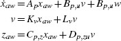
Throughout this chapter, it will be useful to refer to suitable state-space representations of the plant and of the anti-windup compensator dynamics. In particular, assuming that the plant is linear, the following state-space representation will be used:

where xp ∈ ![]() n p is the state, y ∈
n p is the state, y ∈ ![]() n y is the measured output, z ∈
n y is the measured output, z ∈ ![]() n z is the performance output, σ ∈
n z is the performance output, σ ∈ ![]() n u is the control input, and w is the external input gathering references and disturbances. Moreover, since the anti-windup filter F is based on a model of the plant from the input u to the output y, it will have the following state-space representation:
n u is the control input, and w is the external input gathering references and disturbances. Moreover, since the anti-windup filter F is based on a model of the plant from the input u to the output y, it will have the following state-space representation:

The anti-windup closed loop then corresponds to the interconnection of (7.1), (7.2) and the unconstrained controller via the anti-windup interconnection equations
where uc is the measurement input and yc is the output of the unconstrained controller. It follows that the anti-windup compensator (7.2) can be written in the equivalent form

The stability and performance properties induced by MRAW on the closed loop depend on the choice of the feedback signal v. Because of the cascaded structure described in Figure 6.2 on page 159, this signal performs a stabilizing action aimed at driving the actual plant response toward the (ideal) unconstrained responses whose information is captured through the extra dynamics of the anti-windup filter. The MRAW scheme of Figure 7.1 allows for very general selections of the compensation signal v, ranging from linear to nonlinear and sampled-data ones. The natural starting point for the selection of v is the linear feedback
which can be written equivalently as
or
All the linear MRAW algorithms given in this chapter correspond to selecting the linear gains K and L in (7.5) according to different procedures with certain applicability and expected performance. All of them will be specified by giving the final selection for K and L in the compensation scheme given by (7.2), (7.3), (7.5). However, it is useful to emphasize up front that the scheme is fully equivalent to the implementation (7.4), (7.3), (7.5) and also fully equivalent to the use of an external linear anti-windup compensation filter F driven by sat(u) - u as in Section 2.3.6 on page 34 and having state-space representation
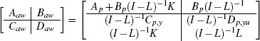
whose output is partitioned in two signals, the first one to be added to the unconstrained controller input and the second one to be added to the unconstrained controller output as indicated in Section 2.3.6. These expressions were given in Section 6.3.3 as well.
The rest of this chapter is dedicated to prescriptive algorithms for generating the feedback matrices K and L. When L ≠0, the equation (7.5), or any of its equivalent forms, contains an algebraic loop that must be solved during implementation. All of the algorithms in this chapter guarantee that this algebraic loop is well-posed.
In Section 7.2, LMI-based synthesis algorithms will be provide for which global stability and performance are guaranteed. These algorithms are not applicable to closed-loop systems with unstable plants. For exponentially stable plants, they do not require a priori information about the size of the disturbances acting on the system. The performance induced by these algorithms can be too conservative for small to medium disturbances. On the other hand, sometimes these algorithms still perform quite well over all disturbance levels.
In Section 7.3, LMI-based synthesis algorithms for regional stability and performance will be provided. These algorithms are applicable to any closed-loop system, but the region over which the algorithms may be applied is limited when the plant is exponentially unstable. Moreover, information about the size of the disturbances acting on the system is required if guarantees on performance are required.
7.2 GLOBAL STABILITY-BASED ALGORITHMS
7.2.1 Global exponential stability
When seeking for global guarantees, a straightforward strategy for selecting the compensation signal v is given by the following Lyapunov-based procedure, where the degrees of freedom available in the design process can often lead to good performance, even though this should be tuned by means of trial-and-error approaches. First the case where the plant is exponentially stable will be addressed and then a generalization of the algorithm will be introduced that also applies to the case when the plant is stable, but not exponentially (namely, it has single poles on the imaginary axis).
The following algorithm requires two parameters to be chosen before being applied. One of them is the positive definite matrix Q, which has an impact on the way the different states of the plant are weighted within the control action. The second one is the positive scalar factor ρ, which is proportional to the aggressiveness of the stabilizing action.
Algorithm 10(Stability-based MRAW for exponentially stable plants)

Comments: Special cases include IMC anti-windup and Lyapunov-based anti-windup, neither of which creates an algebraic loop. Global exponential stability is guaranteed but no performance measure is optimized.
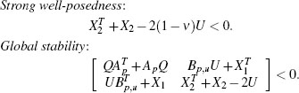
Step 1. Select a constant v > 0 used to enforce a strong well-posedness condition.
Step 2. Solve the following LMI feasibility problem in the free variables Q = QT >0, U >0 diagonal, X 1 and X 2, where X 1 has the same dimension as K and X 2 has the same dimension as L :
Step 3. Using a feasible solution from the previous step, compute the compensation gains as follows:
Step 4. Construct the anti-windup compensation as (7.2), (7.3), (7.5) with the selection (7.9). Equivalently, use the filter (7.8) in an external linear anti-windup compensation scheme.
7.2.1.1 Special classes of feasible solutions
In Algorithm 10, there is no hope of the synthesis LMIs being feasible unless Ap is exponentially stable. When Ap is exponentially stable, there are some obvious solutions to the synthesis LMI.
IMC: One can take X 1 = 0, X 2 = 0, U = I, and Q = ρP –1, where ρ > 0 is sufficiently large and P> 0 satisfies ApTP + PAp > 0. Such a matrix P will always exist when Ap is exponentially stable. These choices lead to picking K = 0 and L =0 in (7.9). In this case, F corresponds to a copy of the plant P. This fact leads to the label “internal model control,” or IMC for short.
Lyapunov-based synthesis: One can take X 1 = —UBTp, X 2 = 0, U > 0 diagonal, and Q =P–1, where P >0 satisfies ApTP + PAp > 0. These choices lead to picking K =—UBTpP, where U is an arbitrary positive definite, diagonal matrix and L =0 in (7.9). Despite its simplicity, in many cases Algorithm 10 with these particular choices is suficiently good to induce highly desirable responses on the resulting closed-loop system.
The following examples illustrate this technique and compare it to the IMC approach.
Example 7.2.1(MIMO academic example) Consider a two-dimensional MIMO plant modeled by the following set of equations:

where sat1 (·) and sat2(·) range between —3 and 3 and —10 and 10, respectively. At time t =0, the outputs x 1 and x 2 are subject to pulse setpoint changes of duration 5 seconds and magnitudes 0.6 and 0.4 respectively. The following PI controller can be used to guarantee zero steady-state error to step references:

where ysp1 and ysp2 represent the setpoints for the outputs.
The two variants of Algorithm 10 can be applied to this academic example:
1. For the IMC approach, nothing needs to be computed: since Ap is exponentially stable (all the eigenvalues have a negative real part), the anti-windup compensation is feasible and corresponds to the selection K =0 and L =0 in (7.2), (7.3), (7.5).
2. For the Lyapunov-based synthesis, the matrix p is selected as the solution of the Lyapunov equation ApTP +PAp =—Q,Q =0.2I >0. Picking U =I, the solution then becomes:
to be used in (7.2), (7.3), (7.5).
Different responses to the pulse references described above are reported in Figures 7.2 and 7.3, where the two outputs and the two inputs of the plant are represented, respectively. In particular, the dashed curves represent the unconstrained response, which exhibits desirable behavior. The dotted curves, which exhibit an unstable behavior, correspond to the response of the saturated system. The dashed-dotted curves represent the response of the IMC anti-windup and the solid curves represent the response of the Lyapunov-based anti-windup.
While the saturated system exhibits instability, IMC anti-windup is at least able to recover closed-loop stability, but the associated performance is very sluggish: it takes an awfully long time for the dashed-dotted IMC response in Figure 7.2 to converge to the unconstrained dashed response. A much more desirable behavior is exhibited by the Lyapunov-based anti-windup (solid curves in Figure 7.2), which, by way of a nonzero selection of the compensation signal v, is able to force the output response back onto the unconstrained one. The corresponding transients happen in the first 0.5 seconds and are almost invisible in Figure 7.2. They can, however, be appreciated in the lower plot of Figure 7.3, where it appears that the anti-windup system is making use of the second input to quickly “recover” the unconstrained performance. ![]()

Figure 7.2 Plant output responses of various closed loops for the MIMO academic example in Example 7.2.1.

Figure 7.3 Plant input responses of various closed loops for the MIMO academic example in Example 7.2.1.
Example 7.2.2 (A turbofan engine) Consider the following turbofan engine model which has three states, three inputs, and three performance outputs (all of them available for measurement):
where

The eigenvalues of Ap are -4. 4615, – 2. 8055, and -0.1375; hence, the plant is open-loop stable. The three outputs y ∈ ![]() 3 to be controlled are the fan speed (PCN2R), the core engine pressure ratio (CEPR), and the liner engine pressure ratio (LEPR), respectively. The three inputs u ∈
3 to be controlled are the fan speed (PCN2R), the core engine pressure ratio (CEPR), and the liner engine pressure ratio (LEPR), respectively. The three inputs u ∈ ![]() 3 are the fuel flow rate (WF), the nozzle area (A8), and the bypass duct area (A16), respectively.
3 are the fuel flow rate (WF), the nozzle area (A8), and the bypass duct area (A16), respectively.
With the primary goal of guaranteeing decoupled tracking of the set points for PCN2R and CEPR with good regulation of LEPR, the following unconstrained controller has been derived for the unconstrained system:
where ysp ∈ ![]() 3 is the setpoint value for the outputs and the matrix entries are:
3 is the setpoint value for the outputs and the matrix entries are:

Three of the eigenvalues of Ac are–0.002, while the fourth one is–0.1476. This suggests that the unconstrained closed-loop system may be subject to windup. Indeed, slow modes in the unconstrained controller often lead to poor performance in the presence of saturation.
The two variants of Algorithm 10 can be applied to the turbofan engine:
1. For the IMC approach, nothing needs to be computed: since Ap is exponentially stable (all the eigenvalues have a negative real part), the anti-windup compensation is feasible and it corresponds to the selection K =0 and L = 0 in (7.2), (7.3), (7.5).
2. For the Lyapunov-based synthesis, the matrix P is selected as the solution of the Lyapunov equation ApTP +PAp = –Cp,yTCp,y >0, where the inequality holds because C p,y is a full-rank matrix. Picking U =I, the solution then becomes:

to be used in (7.2), (7.3), (7.5).

Figure 7.4 Plant output responses of various closed loops for the turbofan example in Example 7.2.2.
For the turbofan engine, a simulation setup is studied where the output set point (or the reference input) is a pulse of amplitude 1.5 and duration 2 seconds at the PCN2R reference input. All the inputs are assumed to be constrained between ±1.5. Figures 7.4 and 7.5 represent the closed-loop responses of the unconstrained system (dashed), the saturated system (dotted), the anti-windup closed-loop system with IMC compensation (dashed-dotted), and the anti-windup closed-loop system with Lyapunov-based compensation (solid).

Figure 7.5 Plant input responses of various closed loops for the turbofan example in Example 7.2.2.
From the simulations it appears that IMC anti-windup already does better than the saturated response especially in the second portion of the simulation. Lyapunov-based compensation is capable of improving even more the output response at the first output (top plot of Figure 7.4) by better exploiting the input authority available on all three inputs (see the middle and lower input plots in Figure 7.5. This ability of the anti-windup compensation to exploit as much as possible the input authority to recover as soon as possible the unconstrained output performance is the key feature that makes it desirable in many practical situations. ![]()
7.2.2 Global asymptotic stability
As shown in the previous example, designing the compensation signal v in (7.5) only based on the matrix K (namely, constraining L =0) and selecting this matrix based on a simple Lyapunov argument can already lead to high-performance solutions to the anti-windup problem. A useful generalization of Algorithm 10 is represented by the construction described in this section. The main advantage of this generalization as compared to the previous algorithm is that it also applies to plants which contain marginally stable modes (in addition to possible exponentially stable ones). Marginally stable modes correspond to single poles on the imaginary axis. This class of systems is quite common in real applications because it corresponds to the case of linear (or possibly linearized) mechanical systems without friction forces, where typically the state is formed by positions and velocities of geometrical coordinates, and each degree of freedom characterizes a single pole at the origin.
The dynamics of stable plants with possible marginally stable modes correspond to a state-space representation where the Jordan canonical form of the state transition matrix doesn't have Jordan blocks of size greater than one for any of the eigenvalues on the imaginary axis. To suitably describe the construction algorithm, it will be useful to transform the state-space representation of the plant model reproduced in the MRAW filter into the following form:
where A0 is a block diagonal matrix characterizing all the marginally stable modes of the plant and, consequently, As is exponentially stable. In particular, if a certain marginally stable mode of the plant is real, then the corresponding entry on the diagonal of A0 will be a “0.” On the other hand, if the marginally stable mode is a pair of complex conjugate poles, then the entry will be a submatrix of the form ![]() . This can be done according to the following procedure.
. This can be done according to the following procedure.
Procedure 5(State-space transformation for marginally stable plants)
Step a) Define two matrices Ap and Bp such that all the eigenvalues of Ap have a nonpositive real part and all the eigenvalues on the imaginary axis have algebraic multiplicity equal to the geometric multiplicity (namely, they are single poles).
Step b) Compute the Jordan form Jp of Ap and the coordinate transformation matrix TJ such that T–ljApTJ = Jp (this can be done in a simple automated way using, e.g., the MATLAB command [Tj, Jp] =jordan(Ap)). The matrix Jp will have all the eigenvalues of Ap on its main diagonal. Denote by n0 the number of (single) eigenvalues on the imaginary axis and by ns the number of the remaining eigenvalues.
Step c) Construct the matrix T0 column by column as follows:
1. for each column of TJ corresponding to a real eigenvalue in Jp leave that column unchanged; for each pair of complex conjugate columns in TJ corresponding to a pair of complex conjugate eigenvalues in Jp replace that pair with two real columns corresponding to the real and the imaginary part of any of the two complex conjugate columns of TJ;
2. stack in T0 the columns corresponding to eigenvalues in jp with strictly negative real part first; then complete T0 with all the columns related to eigenvalues in jp with zero real part.
Step d) Define the transformed state-space representation for the MRAW compensator matrices as ![]()
![]()
The following example illustrates, for a nontrivial case, the use of Procedure 5 to transform an anti-windup compensator with neutrally stable modes into the form (7.13).
Example 7.2.3Consider the MRAW compensator (7.2) with the following selections:

(note that the other matrices in (7.2) are not relevant to the purpose of this example). Step b of Procedure 5 consists in computing the Jordan form Jp of Ap and the coordinate transformation matrix TJ such that TJ-1ApTJ = Jp. The resulting matrices are the following:

from which it is evident that Ap has a neutrally stable pole at the origin and a pair of complex conjugate neutrally stable poles at ±20i. To obtain from Tj a coordinate transformation that generates the block matrix in (7.13), according to step c, it suffices to first replace all the pairs of complex conjugate eigenvectors with the corresponding real and imaginary parts and then to reorder the columns of Tj so that the eigenvectors corresponding to the neutrally stable modes of Ap appear in the last columns of T0. The resulting transformation matrix T0, the resulting block diagonal matrix ![]() p = T0–1ApT0,and the corresponding input matrix
p = T0–1ApT0,and the corresponding input matrix ![]() are the following:
are the following:

which complies with the representation required. Note that since in equation (7.13) the matrix As is a generic matrix, the first columns in the transformation matrix T0 can be permuted and/or transformed by linear combinations (as long as they preserve the linear independence of the resulting columns). This will result in a non-diagonal matrix As which may correspond to a more desirable representation of the anti-windup compensator dynamics. ![]()
After having clarified that any anti-windup compensator with simple, neutrally stable poles can be represented in the form (7.13), it is possible to proceed with the description of the anti-windup construction algorithm. In the next algorithm, there are three free design parameters. Two of them, consisting in a positive definite matrix Qs having the same size as As and a positive scalar ρ, represent the generalization of the design parameters in step 1 of Algorithm 10. A third one, consisting in another positive scalar p 0, allows weighing the control authority devoted to the stabilization of the neutrally stable modes, as compared to that devoted to the overall anti-windup action.
Algorithm 11(Lyapunov-based MRAW for marginally stable plants)

Step 1. Verify that the anti-windup matrices are in the form (7.13), otherwise perform a change of coordinates, following Procedure 5.
Step 2. Select a positive definite matrix Qs of the same size as As, and positive scalars ρ, ρ 0.
Step 3. Solve the following Lyapunov equation:
in the free variable Ps >0 (for example, use the MATLAB command Ps = lyap(As’, Qs)).
Step 4. Construct the block diagonal matrix
where I0 is the identity matrix of the same size as A0.
Step 5. Select the compensation gains as L =0 and K = –ρBTP.
Step 6. Construct the anti-windup compensation as (7.2), (7.3), (7.5) with the selection at the previous step. Equivalently, use the filter (7.8) in an external linear anti-windup compensation scheme.
![]()
The proof of the effectiveness of the construction in Algorithm 11 actually allows for any selection for v of the form given at step 5, where P is a positive definite matrix that solves the Lyapunov inequality
However, in general, this solution cannot be determined in a straightforward way, and Algorithm 11 provides a constructive procedure to select such a matrix P.
Similar to the case of Algorithm 10, when the plant has more than one input, the constant ρ can be replaced by an arbitrary positive definite diagonal matrix to allow for extra degrees of freedom in affecting the plant inputs. Moreover, the constant ρ0 can be selected as a diagonal positive definite matrix, to allow for different weighting on the different neutrally stable modes. However, special care has to be taken to ensure that for each pair of complex conjugate neutrally stable eigenvalues, the corresponding entries on the diagonal matrix coincide, otherwise the resulting matrix P constructed at step 4 won't satisfy the necessary condition (7.14).
Example 7.2.4(SISO academic example) Consider the the SISO academic example qualitatively discussed in Section 1.2.1 on page 4. The plant consists of a simple integrator with an additive input disturbance. The corresponding matrices in (7.1) are
where ![]() comprises the reference and disturbance inputs. For this example, a PID controller is used with all the gains equal to one to induce a desirable closed-loop response and suitable disturbance rejection. The controller can be any type of approximate PID controller as its implementation makes little difference on the resulting closed loop. In addition, the anti-windup compensation acts before and after the controller and is controller independent. The control input in the unconstrained case is selected as the difference r– y, which is also taken as the performance output, namely,
comprises the reference and disturbance inputs. For this example, a PID controller is used with all the gains equal to one to induce a desirable closed-loop response and suitable disturbance rejection. The controller can be any type of approximate PID controller as its implementation makes little difference on the resulting closed loop. In addition, the anti-windup compensation acts before and after the controller and is controller independent. The control input in the unconstrained case is selected as the difference r– y, which is also taken as the performance output, namely,
Following Algorithm 11, the plant dynamics is already in the form (7.13) because it contains only one pole at the origin. Therefore, it is not necessary to apply Procedure 5. At step 2, As and Qs are empty matrices and the selection ρ =ρ0 = 1 is chosen. Then the algorithm provides the selection L 0, K–1. Anti-windup compensation is designed by augmenting the closed loop with the MRAW filter (7.2), (7.3), (7.5) and with this selection.
The simulation of Figure 7.6 is performed by limiting the control input between ±0.1 and selecting the following reference and disturbance inputs:
namely, unit step reference applied at time t = 0 and an impulsive disturbance occurring at time t = 80.
From the simulation it appears that the anti-windup solution (solid) allows recovering as quickly as possible the unconstrained response (dashed) and eliminating the undesirable windup-induced oscillations exhibited by the saturated closed loop (dotted). ![]()

Figure 7.6 Plant input and output responses for the SISO academic example in Example 7.2.4.
Example 7.2.5. Consider the servo-positioning system introduced in Section 1.2.4 on page 10 and represented in Figure 1.10. The design qualitatively illustrated in that section is described in greater detail here.

Figure 7.7 Coordinates of the servo-positioning system.
A coordinate system can be defined on the system, as represented in Figure 7.7, where the point p0 corresponds to p = 0, the point pA corresponds to p = –1, and the point pB corresponds to p = 1. Assuming that the mass is actuated by an electrical motor, if the arc length of the path represented in Figure 7.7 (namely, distance traveled along the path) is approximated with the horizontal coordinate, then the linear transfer function of the plant can be written as
where τM = 2s is the mechanical time constant of the motor and of the cart, and FL(s) is the load torque arising from the gravity action.
To guarantee that the unconstrained closed loop has a 3 dB bandwidth of 6 rad/s and zero steady-state error with constant disturbances, the controller needs to contain a pole in the origin and, based on a frequency domain design, it can be augmented with two coincident lead networks as follows:
where r(s) is the reference representing the desired mass position and F (s) is a feedforward filter that improves the transient response. According to the path profile represented in Figure 7.7, by selecting the maximum load force to be equal to 0.5 N, the disturbance input FL can be chosen as a function of the mass position p, as follows:

Consider the presence of saturation at the plant input, which constrains the force exerted on the mass to be between ±1. The unconstrained closed-loop response of this system when the reference signal corresponds to a step between zero and δ = 0.05 is represented in Figure 1.11, and corresponds to plant inputs that remain smaller than the saturation limits for all times. Hence, the saturated system can reproduce this response. However, the closed-loop system exhibits very different behaviors when the step reference corresponds either to the top of the bounce on the right side (namely, r = 1) or to the bottom of the dip on the left side (namely, r = –1).

Figure 7.8 Responses of the positioning system of Example 7.2.5. when the step reference signal is 1 (upper plot) and –1 (lower plot).
When disregarding input saturation and considering the unconstrained closed-loop responses, these two trajectories are represented by the dashed curves in the two plots of Figure 7.8 (which resemble the responses previously reported in Figures 1.11, 1.12, and 1.14). Note that the effect of the disturbance on the unconstrained closed-loop system is almost negligible. However, the windup effect for this system is very significant, and the saturated response, corresponding to the dotted curves in the same figure, is unacceptable.
To compensate for the undesirable saturated response, an anti-windup compensator can be constructed for this control system according to Algorithm 11 (note that the other algorithms proposed in this chapter and in the previous one are not applicable to this case because the plant is not exponentially stable). To this end, consider the following state-space representation of the plant:

Then, by selecting Qs =1, ρ =50, and p0 = 0.01, the selection in step 5 corresponds to choosing ![]() . The response of the resulting anti-windup closed-loop system is represented by the solid curves in Figure 7.8. Note that the anti-windup action eliminates the windup effects experienced on the dotted responses and guarantees a smooth convergence to the desired steady state (in addition to preservation of the local unconstrained performance).
. The response of the resulting anti-windup closed-loop system is represented by the solid curves in Figure 7.8. Note that the anti-windup action eliminates the windup effects experienced on the dotted responses and guarantees a smooth convergence to the desired steady state (in addition to preservation of the local unconstrained performance).![]()
7.2.3 Global exponential stability with local LQ performance
A natural performance measure that one can consider for the design of the stabilizing signal v is a generic quadratic cost of the form:
With the goal of formulating suitable linear matrix inequalities for anti-windup design, instead of minimizing the linear quadratic (LQ) performance index above evaluated along the real solutions of the anti-windup compensator (7.2), it is possible to minimize it when applied to the solutions of the following linear system:
which, especially for the medium signal setting, well approximate the trajectories of the original system (7.2). Several case studies have shown that the resulting compensation gains often lead to highly desirable performance.
Algorithm 12 (Global LQ-based MRAW)

Step 1.Select two square positive definite matrices QP and RP of the size of the compensator state and of the compensator input, respectively. Select a constant v ∈ [0,1) used to enforce a strong well-posedness constraint (see Section 2.3.7).
Step 2. Solve the following LMI optimization problem, in the free variables Q = QT > 0, U > 0 diagonal, γ > 0, X 1, and X 2, where X 1 has the same dimension as Kv and X 2 has the same dimension as Lv :

Step 3. Based on the optimal solution resulting from the previous step, compute the compensation gains as follows:
Step 4. Construct the anti-windup compensation as (7.2), (7.3), (7.5) with the selection at the previous step. Equivalently, use the filter (7.8) in an external linear anti-windup compensation scheme.
Example 7.2.6 (Damped mass-spring system) The mass-spring system in Figure 7.9 was briefly discussed and introduced in Section 1.2.5 on page 13. It is here described in much more detail. Its equations of motion are given by

where ![]() represents position and speed of the body connected to the spring, m is the mass of the body, k is the elastic constant of the spring, f is the damping coefficient, u represents a force exerted on the mass, and d represents a disturbance at the plant's input. The following values for the parameters can be selected:
represents position and speed of the body connected to the spring, m is the mass of the body, k is the elastic constant of the spring, f is the damping coefficient, u represents a force exerted on the mass, and d represents a disturbance at the plant's input. The following values for the parameters can be selected:

Figure 7.9 The damped mass-spring system.

Figure 7.10 The unconstrained (linear) closed-loop system in Example 7.2.6.
Assume that r ∈ ![]() is a reference input corresponding to the desired mass position. The linear controller shown in Figure 7.10 corresponds to the equations:
is a reference input corresponding to the desired mass position. The linear controller shown in Figure 7.10 corresponds to the equations:
with
This controller has been determined with the aim of guaranteeing a fast response with zero steady-state error to step reference changes, robust to parameter uncertainties. While the performance of the system is very desirable in the absence of saturation (namely when uc = y and up yc), this control scheme appears to be extremely sensitive to the activation of the saturation nonlinearity.
This is confirmed by the simulations of the unconstrained and saturated closed-loop systems. Consider the case where the disturbance d is chosen as a band-limited white noise of power 0.001 passed through a zero-order holder with sampling time 0.001 seconds. The response of the unconstrained closed-loop system starting from the rest position and with the reference switching between ±0.9 meters every 5 seconds and going back to zero permanently after 15 seconds is shown by the dashed curve in Figure 7.11. When the force exerted at the plant's input u is limited to between ±1 kg • m/s2, the corresponding saturated closed-loop response, represented by the dotted curve in Figure 7.11, exhibits persistent oscillations between positive and negative peaks qP ≈ 370 meters.
To address and solve this windup problem following the construction proposed in Algorithm 12, the parameters at step 1 are selected as:
and v = 0.1. Moreover, to improve the numerical conditioning of the LMI solver, the value of the scalar L has been constrained between ±1 by adding the extra LMI–2U > X 2 + X 2T. This LMI combines with X 2 + X 2T > 2 U (which comes from the lower right term in the global stability LMI at step 2) to imply |L| > 1. Note that this trick only works for the case of L being a scalar and otherwise only guarantees a bound on the symmetric part of L suitably scaled by the diagonal matrix U. The following solution to the LMI optimization problem at steps 2 and 3 is obtained:

Figure 7.11 Various closed-loop responses for the mass-spring system in Example 7.2.6.
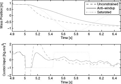
Figure 7.12 An enlarged version of the responses reported in Figure 7.11.
The resulting anti-windup response corresponds to the solid curve in Figure 7.11. An enlarged version of the initial transient is shown in Figure 7.12 to better illustrate the anti-windup trajectory and its difference from the unconstrained one. ![]()
7.2.4 Global exponential stability with local H2 performance
An interesting viewpoint for designing the anti-windup compensation gains in (7.5) arises from the observation that, as clarified in Section 6.2, by virtue of the action of the signal yaw, the input of the unconstrained controller always coincides with the unconstrained plant response. Therefore, its output yc also always coincides with the controller output in the unconstrained closed loop. Moreover, in many cases the controller output in the unconstrained closed loop converges to small values after a reasonably short time because it is a signal generated by a linear closed-loop system which is designed to guarantee high performance, and this usually corresponds to imposing fast transients and fast convergence to the steady state. On the other hand, looking at the anti-windup compensator structure (7.2), it appears evident that the controller output yc acts as a disturbance on the anti-windup dynamics. Hence, in all the cases described above, it can be thought of as a pulse which rapidly drives the state xaw far from the origin and then converges back to zero or to a steady-state value which is smaller than the saturation levels.
It is then of interest to minimize the integral of the performance output zaw = z– zi by guaranteeing that this integral be smaller than the size of the initial state xaw of the anti-windup compensator dynamics, suitably scaled by a variable γ2 which measures the anti-windup performance level. Moreover, since the signal yc affects the dynamics (7.2) through the input matrix Bp,u, it may be convenient to consider in the optimization problem only the initial conditions that belong to the image of the matrix Bp,u, because this corresponds to the region where the anti-windup state xaw will be forced into, after a pulse drives the compensator from the input yc.
More precisely, the following algorithm seeks for selections of K and L in (7.5), aimed at minimizing the quantity γ2 in the following inequality:
where T is the smallest time such that sat(ui(t)) = ui(t) for all t≥T, and where xaw(T) belongs to the image of the matrix Bpu.
The abovementioned performance measure corresponds to the H 2 norm of the system
from the input w to the output zaw. This is the motivation for the name given to this particular MRAW construction algorithm.
The algorithm involves the selection of a free design parameter ρv≥ 0. This scalar penalizes the size of the matrices K and L, for implementation purposes. Indeed, especially in the case where Dp, zu = 0, by selecting ρv = 0, the convex optimization procedure might result in very high values of K and L, while selecting ρv to be a small positive number makes the matrix sizes reasonable at the price of a negligible reduction of the performance level.
Algorithm 13(Global H2–based MRAW)

Step 1. Select a nonnegative constant ρv≥ 0, constituting a penalty on the matrices K and L. Select a constant v ∈ [0,1) used to enforce a strong well-posedness constraint (see Section 2.3.7).
Step 2. Solve the following LMI optimization problem, in the free variables Q = QT> 0, U> 0 diagonal, j> 0, X 1, and X 2, where X 1 has the same dimension as K and X 2 has the same dimension as L :

Step 3. Given the optimal solution resulting from the previous step, compute the compensation gains as follows:
Step 4. Construct the anti-windup compensation as (7.2), (7.3), (7.5) with the selection at the previous step. Equivalently, use the filter (7.8) in an external linear anti-windup compensation scheme.
Note that for the algorithm to be completed, the matrix in the brackets at step 3 needs to be nonsingular. Nonsingularity of this matrix can indeed be guaranteed based on the properties of the LMI constraints at step 2.
The matrix Bp,u appearing in the off-diagonal term of the last LMI at step 2 corresponds to the set of initial conditions for which the H2 performance is minimized. In some cases it might be convenient to replace this matrix with an identity so that the H2 performance from any initial condition is minimized. Otherwise, alternative subspaces of initial conditions that are of interest for the anti-windup problem under consideration can be incorporated in the optimization constraints by suitably replacing that off-diagonal term.
7.3 REGIONAL STABILITY AND PERFORMANCE ALGORITHMS
7.3.1 Regional LQ-based design
With the goal in mind of only guaranteeing regional results, a very simple selection for the anti-windup gains in (7.5) consists in selecting L = 0, so that no algebraic loops will arise in the scheme, and in selecting K as a stabilizing state feedback gain for the simplified dynamics
that corresponds to the actual anti-windup dynamics (7.2) for small enough signals (namely, when saturation is not active) and well approximates the anti-windup dynamics as long as v remains sufficiently small.
Any stabilizing K will guarantee regional stabilization, but since saturation is not taken into account in the design phase, the stability region of the anti-windup closed-loop system may as a result be too small, especially when K is very aggressive. Nevertheless, within this family of solutions, a design paradigm that has proven to work well in practice consists in selecting the gain K as a stabilizing gain via an LQ design, as detailed in the next algorithm.
Algorithm 14(Regional LQ-based MRAW)

Step 1.Select two weight matrices Q = QT≥ 0 and R = RT≥ 0 for the anti-windup state and input variables.1
Step 2.Choose the anti-windup gain K as an LQR gain with weights (Q, R) (e.g., use the MATLAB command K=-lqr (A,B,Q,R)). Choose L = 0.
Step 3.Construct the anti-windup compensation as (7.2), (7.3), (7.5) with the selection at the previous step. Equivalently, use the filter (7.8) in an external linear anti-windup compensation scheme.
Example 7.3.1(Damped mass-spring system) Consider once again the damped mass-spring system studied in Example 7.2.6 on page 190. In that example, the compensation gains were selected by following Algorithm 12, which can be well understood as the equivalent of Algorithm 14 when global closed-loop stability guarantees are desired.

Figure 7.13 Various closed-loop responses for the mass-spring system in Example 7.3.1
Since no closed-loop stability is ensured by Algorithm 14, it is expected that a more aggressive compensation law will be obtained, possibly inducing a better performance but at the risk of destabilizing the plant in some situations. For this example, by selecting the parameters at step 1 of Algorithm 14 to be ![]() and R = 1, the gain K = [-21.38 -3.78] is obtained, which leads to an extremely desirable closed-loop response. The closed-loop response with this anti-windup compensator is compared to the unconstrained (dashed), saturated (dotted) and global LQ anti-windup responses in Figure 7.13, which reports on the equivalents of the two top plots of Figures 7.11 and 7.12 when using Algorithm 14. From the curves in Figure 7.13 it is quite evident that this example greatly benefits from the use of the regional compensation scheme. It should be kept in mind, however, that only local stability guarantees hold when using this scheme.
and R = 1, the gain K = [-21.38 -3.78] is obtained, which leads to an extremely desirable closed-loop response. The closed-loop response with this anti-windup compensator is compared to the unconstrained (dashed), saturated (dotted) and global LQ anti-windup responses in Figure 7.13, which reports on the equivalents of the two top plots of Figures 7.11 and 7.12 when using Algorithm 14. From the curves in Figure 7.13 it is quite evident that this example greatly benefits from the use of the regional compensation scheme. It should be kept in mind, however, that only local stability guarantees hold when using this scheme. ![]()
7.3.2 Regional H2 -based design
Based on the global H2 based MRAW approach of Section 7.2.4, a possible strategy to design the compensation gains K and L for regional results is to follow that same construction and, instead of guaranteeing global exponential stability by constraining the nonlinearity in the global sector, using the regional sector tools in Section 3.5 to obtain extra degrees of freedom in the design phase and only regional guarantees. Based on that regional sector property, it is desirable to solve an optimization problem minimizing γ2 in (7.21) by requiring stability guarantees in only a subset of the state space corresponding to an ellipsoid characterized by a sublevel set of a Lyapunov function denoted by ε(P)={xaw : xawTPxaw ≥ 1}. Then, stability would only be guaranteed in a bounded subset of the state space but the anti-windup compensation performance would in general be improved. In addition to this, similar to the previous section, these regional constructions can be applied to any linear windup-prone control system because focusing on a bounded set still leaves enough input authority to make the stability LMIs feasible for any type of plant (rather than only being feasible for exponentially stable plants, as it was the case for the global Algorithm 13).
The next algorithmpursues the goal referred to above. The algorithmrequires the selection of three design parameters, one of them being the strong well-posedness parameter v (see Section 2.3.7), the second one being a desired guaranteed stability region, characterized by a matrix Ps so that ξ(Ps) is certainly in the domain of attraction, and the third one, ρv, being a penalty term for the matrices K and L paralleling the one introduced in the global Algorithm 13.
Since the algorithm relies on the use of the regional sector tools of Section 3.5, it involves the knowledge of the saturation levels ![]() i > 0, i = 1,…, nu, which may all be different from each other. Due to the properties of those sector tools, the quantities
i > 0, i = 1,…, nu, which may all be different from each other. Due to the properties of those sector tools, the quantities ![]() i > 0 only need to be lower bounds on the saturation levels which could be time-varying and/or nonsymmetric. Note, however, that, as extensively commented on in Chapter 6, the problem of designing v in the MRAW compensation scheme is a transformed problem where the saturation nonlinearity is shifted by the presence of the signal yc. Therefore, when dealing with setpoint stabilization problems, one could consider restricting the values
i > 0 only need to be lower bounds on the saturation levels which could be time-varying and/or nonsymmetric. Note, however, that, as extensively commented on in Chapter 6, the problem of designing v in the MRAW compensation scheme is a transformed problem where the saturation nonlinearity is shifted by the presence of the signal yc. Therefore, when dealing with setpoint stabilization problems, one could consider restricting the values ![]() i by an amount corresponding to the worst case steady-state controller output yc, given a bound on the allowable reference signals. In this way, the (regional) stability guarantees of the next algorithm will hold for all references satisfying that bound.
i by an amount corresponding to the worst case steady-state controller output yc, given a bound on the allowable reference signals. In this way, the (regional) stability guarantees of the next algorithm will hold for all references satisfying that bound.
Algorithm 15(Regional H2-based MRAW)

Step 1.Select a symmetric matrix Ps associated with a desired guaranteed stability region ε(Ps) := {xaw : xTawPsxaw 1}. Select a nonnegative constant ρv ≥ 0, for a penalty on the matrices K and L. Select a constant v ∈ [0,1), used to enforce a strong well-posedness constraint (see Section 2.3.7).
Step 2. Solve the following LMI optimization problem, in the free variables Q = QT> 0, U> 0 diagonal, γ > 0, Y, X 1, and X x2,where X1 and Y have the same dimension as K and X2 has the same dimension as l :

where Yi denotes the i th row of the matrix Y and where ![]() 1,….
1,…. ![]() nu denotes the symmetric saturation limits.
nu denotes the symmetric saturation limits.
Step 3. Given the optimal solution resulting from the previous step, compute the compensation gains as follows:
Step 4. Construct the anti-windup compensation as (7.2), (7.3), (7.5) with the selection at the previous step. Equivalently, use the filter (7.8) in an external linear anti-windup compensation scheme.
![]()
Note that for the procedure to be completed, the matrix in the brackets at step 3 needs to be nonsingular. Similar to the preceding Algorithm 13, this matrix is guaranteed to be invertible by the properties of the LMI constraints at step 2.
The IMC anti-windup scheme seen as a special case of Algorithm 10 is a reinterpretation (see the notes and references of Chapter 6) of the IMC anti-windup first described in [G21] and then well characterized in [FC7]. The Lyapunov-based synthesis seen as a special case of the same algorithm was suggested in [MR3] for global stability and was there applied to Example 7.2.1 using the gains reported here. The synthesis of Algorithm 11 for global asymptotic stability for marginally stable plants also derives from the ideas in [MR3] and has been illustrated in more detail in the application paper [AP10], where also its discrete-time counterpart is discussed. The global LQ-based synthesis LMIs given in Algorithm 12 come from [MR15], while the regional LQ-based approach is a natural extension of the results in [MR3]. The global and regional H2-based designs of Algorithms 13 and 15, respectively, come from the ideas in [MR21], even though a different sector characterization was used for the regional design therein proposed. Here, in contrast to [MR21], the LMIs for regional performance follow from the ideas presented in Section 3.5 of Chapter 3, which come from [SAT11] and [MI27].
The plant model used in the MRAW compensation architecture can be an approximated model, and the intrinsic robustness of the scheme guarantees a certain level of tolerance with respect to unmodeled dynamics. See [MR31] for a discrete-time case study with reduced-order models.
The MIMO academic example treated in Example 7.2.1 was introduced in [CS7] and later revisited in [MR3] to illustrate the MRAW construction discussed in this chapter. The turbofan engine example in Example 7.2.2 is taken from [AP1], where details can be found on the design of the unconstrained controller. Moreover, in [AP1] the solution presented here is compared to the use of the conditioning technique from [FC6]. Finally, [AP1] also reports an interesting discussion on the projection of in-feasible references onto feasible ones while preserving certain performance requirements. The SISO academic system of Example 7.2.4 was used by Åström in [CS2] while Example 7.2.5. was cooked up by the authors of this book to illustrate how disturbances can lead to windup effects. The damped mass-spring system in Examples 7.2.6 and 7.3.1 was introduced in [MR15] and later used in many anti-windup papers (see, e.g., [MI23, MR23, MR27, MR28]).
1The matrix Q should be selected in such a way that the resulting LQ control law is stabilizing (e.g.,
Q =CTC with (A,C) detectable).