
Chapter Nine
The MRAW Structure Applied to Other Problems
9.1 RATE- AND MAGNITUDE-SATURATED PLANTS
When dealing with plants with both input rate and magnitude saturation, the model recovery anti-windup (MRAW) scheme can be employed to recover the performance of a controller synthesized for the system without input magnitude and rate saturation. From a mathematical viewpoint, input rate saturation can be modeled by augmenting the plant equations, reported here for completeness,
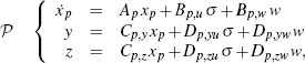
with an additional state equation having the same size as the control input and associated with the following discontinuous dynamics for the new state variable σ:
where u is the input before saturation, sat (·) denotes the input saturation, and σ is the rate-saturated input that becomes part of the augmented state of the plant. Finally, R is a diagonal matrix having as diagonal entries the maximal rates ![]() r,1,…,
r,1,…, ![]() r,nu of each input.
r,nu of each input.

Figure 9.1 The MRAW scheme for rate- and magnitude-saturated systems.
When dealing with magnitude- and rate-saturated inputs, the MRAW scheme can be easily generalized by using the same anti-windup interconnection adopted in the magnitude-saturated case, namely,
where satMR is a shortcut to denote a complicated nonlinear and dynamic effect comprising both magnitude and rate saturation. Moreover, the structural interconnection of the anti-windup compensator is preserved, namely, its input is the difference between the plant input and the unconstrained controller output:

This compensation scheme is represented in Figure 9.1. The only difference compared to the MRAW scheme for magnitude saturation discussed in Chapter 6 and in subsequent chapters lies in the more complicated nonlinearity affecting the plant input. The bottom line is that while the model recovery properties of the MRAW scheme in Figure 9.1 remain the same as those discussed in Section 6.3.2 for the magnitude-saturated case, the mismatch equation (6.14) that is to be stabilized via the feedback signal v becomes now:
so that extra care has to be taken in designing v.
In light of this, most of the algorithms for the design of v discussed in Chapters 7 and 8 cannot be used with rate and magnitude saturation because they don't account for the rate-saturated input. In general, designs for v which are linear functions of the anti-windup state xaw and input (σ - yc) are not sufficient to guarantee global stability or performance results. Nevertheless, the regional design techniques given in Section 7.3 and corresponding to Algorithms 14 and 15 can be used also in the rate-saturated case, where they lead, once again, to regional results. Another solution that works well when the plant is exponentially stable with fast enough modes is the IMC special case of Algorithm 10, which induces global exponential stability but typically poor performance. In the following two examples, the regional linear quadratic (LQ) technique of Algorithm 14 is used to address the windup phenomenon in two relevant flight control systems.
Example 9.1.1 (The Caltech ducted fan) The Caltech ducted fan consists of a short wing and a ducted fan engine with a high-efficiency electric motor and a 6-inch diameter blade, capable of generating up to 15 Newtons of thrust. Paddles on the fan allow the thrust to be vectored from side to side. Additional inputs are the motor speed and the angle of a flap attached to the wing, which acts as an elevator. The engine and wing are mounted on a stand with three degrees of freedom, which allows horizontal and vertical translations as well as an unrestricted pitch angle.
Taking the linearization of the system's dynamics around a trim condition associated with a forward velocity of 8 meters per second, the following model is obtained:
![]()
where the state x ∈ ![]() 6 and the input u ∈
6 and the input u ∈ ![]() 3 represent the following physical quantities:
3 represent the following physical quantities:

The nominal trim condition associated with a forward velocity of 8 meters per second is given by

and the associated system matrices are given by 1.1

A challenging problem associated with the Caltech ducted fan is that the second and the third control inputs are subject to rate saturation, imposed by the maximal velocity of the paddle and of the elevator. Indeed, these devices are also subject to magnitude saturation but the problems induced by the rate saturation are typically more harmful in flight control systems. To address the problem, a composite controller based on two LQR designs is synthesized by exploiting the MRAW approach for magnitude- and rate-saturated plants and the construction in Algorithm 14.
For the trim condition (9.6), two linear quadratic regulators have been designed to minimize two performance indexes depending both on the input u − utrim and on the state x − xtrim. The first one leads to an aggressive control action and is chosen to be the unconstrained controller (note that no dynamics are associated with this design, hence the controller state xc is empty). The second design corresponds to an index where the control input is significantly more penalized than the state, thus leading to a less aggressive controller, suitable to be used as the stabilizing action to be used in Algorithm 14 for v. Note that by Algorithm 14, only regional stability is guaranteed by this anti-windup action, however the basin of attraction of the resulting closed-loop system is sufficiently large to guarantee exponential stability under reasonable operating conditions. Based on the discussion above, the unconstrained controller is selected as
where Khi is selected as an LQR gain with weights Qhi = diag{0.1, 20, 10, 0.1, 1, 10} and Rhi = diag{1, 3, 3} and corresponds to

and the stabilizing signal v is selected as
![]()
where Klo is selected as an LQR gain with weights Qhi=diag{0.1, 20, 10, 0.1, 1,10} and Rhi= diag{1, 3, 3} and corresponds to
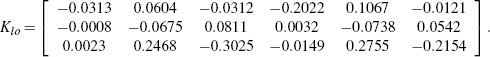
Figure 9.2 reports the simulation results when using a step reference of amplitude 0.5 meters in the vertical displacement (namely, r = [00.50000]T). In the simulation and according to the specifications of the experimental system, the first input is not subject to saturation, and both the second and the third inputs are rate saturated, with a maximal rate of 0.6 rad/s (approximately corresponding to 34.4 deg/s). The top plot of Figure 9.2 shows the vertical displacement output while the middle and lower plots show the two rate-saturated inputs. Notice how the anti-windup response almost recovers the unconstrained performance and eliminates the unpleasant oscillations exhibited by the saturated closed loop.![]()
Example 9.1.2 (The F-16's daisy chain control allocator) The short-period longitudinal dynamics of the VISTA/MATV F-16 at Mach 0.2 and altitude 10,000 feet (corresponding to a dynamic pressure value of 40.8 psf) at a trim angle of attack of 28 degrees is described locally by the linear model
![]() (9.7)
(9.7)
where xp := [αq]T is the state representing deviations of the angle of attack and pitch rate from the trim condition, δ = [δe δptv]T is the input representing respectively the deviations of the elevator deflection and of the pitch thrust vectoring from the trim condition, and the entries of the matrices Ap and Bp,u are:

Figure 9.2 Plant input and output responses of various closed loops for the Caltech ducted fan in Example 9.1.1.
Both inputs are subject to rate and magnitude saturation. By using the model (9.2) for the rate saturation, if u = [ue uptv]T is the input to the saturation block, the following dynamic equations complete the saturated model of the F-16:

where the values Me=21 deg, Mptv = 17 deg, Re = 50 deg/s, Rptv=45 deg/s have been adopted.
According to the results in [SAT4], a daisy-chained allocation of the inputs can be adopted; in particular, if r ∈ ![]() is the desired angle of attack, the desired value for [b21 b22] σ is given by
is the desired angle of attack, the desired value for [b21 b22] σ is given by

According to the matrices in (9.8), the daisy chain allocation is then given by:
Note that, with the above allocation, in the direct connection between the controller and the plant, u = yc, if σptv ≡ ycptv, then [b21 b22] σ ≡ k(x, r); moreover, if σe ≡ yce, then ycptv ≡ 0. In other words, only the elevator deflection input is used to enforce the desired angle of attack.
Following Algorithm 14, the anti-windup compensation signal v is selected by computing a linear gain K optimizing an LQ cost function with Q = 5I2 and R = I2. The resulting gain is
![]()
to be used, according to the algorithm, in v = Kxaw.

Figure 9.3 Plant input and output responses of various closed loops for the F16 case study in Example 9.1.2.
In Figure 9.3, the responses of the unconstrained, saturated, and anti-windup closed loops are compared to each other. The top plot shows the angle of attack and the middle and lower plots represent the two saturated inputs. The reference signal is chosen to be
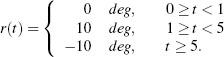
The simulations show that rate limitation induces instability and oscillations. Magnitude limitation is actually reached by the saturated inputs at time t = 9 after the angle of attack has reached a value of 80 degrees, which is definitely already an intolerable flight condition (and is significantly out of scale in the first plot). Anti-windup successfully eliminates the closed-loop instability and induces a desirable closed-loop response slightly deteriorated as compared to the unconstrained one.
![]()
9.2 ANTI-WINDUP FOR DEAD-TIME PLANTS
When a linear plant is subject to the so-called “dead-time” effect—namely it is subjected to a pure delay at its input or, equivalently at its output—the MRAW scheme can be nicely adapted to the situation without much extra effort as compared to the delay-free case. In the most general situation, suppose that there's an input delay τI at the plant control input and an output delay τo at the plant measurement output. The plant equations can be then written as

where the dependence on time has been omitted wherever the functions depend on the current time t.
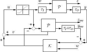
Figure 9.4 The MRAW scheme with dead-time plants.
In this situation, the natural MRAW solution to the windup problem in the presence of input magnitude saturation consists in inserting an identical anti-windup filter to the one used in the delay-free case (see equation (7.4) in Chapter 7.4):

and modifying the interconnection equations as follows
![]()
The block diagram of this compensation scheme is represented in Figure 9.4. The great advantage of this solution is that the delay has been virtually extracted from within the saturation loop and is only left in the loop with delay and without saturation. In other words, the saturation problem has been fully decoupled from the dead-time problem. One way to appreciate this fact is to notice that the model recovery properties of the scheme correspond to the ones discussed in Section 6.2.2 for the delay-free case with the peculiarity that the top system in the cascade representation of Figure 6.2 on page 159 will involve the input and output plant delays, whereas the bottom system, which is affected by saturation, remains the same.
It should be emphasized that due to this fact, the anti-windup problem for dead-time system addresses the problem of recovering the performance of an unconstrained control system which has been designed disregarding actuator saturation but fully taking into account the delay effects. Therefore, the unconstrained closed loop will correspond to the closed loop between the unconstrained controller and the plant without saturation and with delay. No constraints are imposed on the structure of this unconstrained controller indeed, so that, for example, a linear controller equipped with a Smith predictor would satisfy the requirement of being stabilizing for the delayed (but not saturated) plant.
The nice feature of the solution illustrated in Figure 9.4 is that, as in the dead-time free case, the anti-windup problem is transformed into a bounded stabilization problem with disturbances, namely, that of designing v as a suitable linear or nonlinear state feedback signal to drive to zero the state of the dynamics
![]()
which is dead-time free. Due to this reason, almost all the model recovery anti-windup algorithms given in Chapters 7 and 8 can be directly applied to this case, allowing one to address many different situations. An exception to this is Algorithm 23, where extra measurements are required from the plant (namely, the unstable states). That algorithm cannot be generalized to the dead-time case because it would require the availability at time t of the unstable plant states values at time t + tI. This leads to a noncausal solution which requires extra work (e.g., the use of predictors) to be directly applicable.
Example 9.2.1 (An integrating dead-time system) Consider a simple scalar simulation example whose unconstrained closed-loop system is represented in Figure 9.5. The plant is an integrator with a large delay of 5 seconds at its input and the unconstrained controller has a modified Smith predictor structure (the original Smith predictor scheme only applies to exponentially stable dead-time plants).
Since the plant is marginally stable, the construction in Algorithm 11 can be used to design the signal v. In particular, the following state-space representation for the plant can be used:
![]()
and to induce a desirable performance, the parameters in Algorithm 11 are selected as ρ0 = 1, ρ = 10. Therefore the compensation signal is v = -10xaw, where xaw is the only state of the anti-windup compensator. Note that if ρ is increased, a faster performance recovery and more aggressive anti-windup action are obtained.

Figure 9.5 The unconstrained controller for Example 9.2.1.

Figure 9.6 Plant input and output responses of various closed loops for the dead-time system in Example 9.1.1 (nominal case).
Simulation results for the unconstrained, saturated, and anti-windup closed-loop systems are reported in Figures 9.6 and 9.7, where the following selections for the disturbance and reference inputs have been used:
![]()
and a saturation level of ±0.1 is enforced at the plant input.
The first simulation, reported in Figure 9.6 corresponds to the following selection of the parameters of the plant and unconstrained controller of the scheme in

Figure 9.7 Plant input and output responses of various closed loops for the dead-time system in Example 9.1.1 (perturbed case).
![]()
which describes the situation where all the plant parameters are perfectly known and can be incorporated in the unconstrained controller and anti-windup design. In the figure it appears that the anti-windup response (solid) successfully recovers in an efficient way the unconstrained response (dashed). The saturated response (dotted) instead exhibits unpleasant transients. Note also that since the disturbance does not cause input saturation for the unconstrained trajectory, the anti-windup response perfectly reproduces the unconstrained response in the second part of the simulation.
A second simulation is reported in Figure 9.7 where the plant parameters are perturbed by a 10% uncertainty both affecting the unconstrained controller and the anti-windup design. The parameter selection in the scheme in Figure 9.5 then becomes
![]()
Also in this case the anti-windup action is capable of significantly improving the closed-loop response as compared to the saturated case.![]()
9.3 BUMPLESS TRANSFER IN MULTICONTROLLER SCHEMES
Bumpless authority transfer among different controllers is a control goal that was formulated qualitatively in the very early stages of research in applied automatic control. The goal of “bumpless transfer” arose from experimental needs faced by industrialists when the application of classic control techniques led to undesired transients and even instability after power-on and after switching control authority among controllers that induce different closed-loop performance properties.
As an example, due to input saturation, plants are often activated by a preliminary phase where precomputed inputs drive the plant close to the desired operating point (while the automatic controller is still disconnected). Subsequently the controller is switched on and connected to the plant to start the automatic control phase. However, if special care is not taken when interconnecting the controller, the closed loop may experience transients where the plant output reaches unacceptable values and/or the controller output exceeds the saturation limits thus possibly causing stability loss already at power-on. Plant startup is indeed a well-known challenge within the industrial community, especially in the chemical process industry.
Bumpy switches typically correspond to controller-induced transients, after the switch, that unnecessarily affect the plant output and that could be avoided if the controller was appropriately initialized. For this reason, the bumpless transfer problem can be seen as an initial condition problem (for the controller). Indeed, all that matters after switching is that the plant and controller states “match up” and thus lead to a graceful output response where authority is transferred to the controller. Although controller re-initialization is one possible bumpless transfer strategy, alternative approaches, which are typically more robust, correspond to interconnecting the controller to some closed-loop system signals before the switching time (namely, before the time when the controller output is connected to the plant input) using a pre-conditioning scheme that suitably drives the controller dynamics into a safe configuration, ready for the switch. This is the nature of many solutions proposed in the literature, and it is the nature of the approach proposed here.
In the literature, the bumpless transfer problem is often addressed in conjunction with the anti-windup problem. The association between the two problems is mainly motivated by the two following facts. 1) The bumpless transfer problem can be seen as a problem of input substitution, whereas the anti-windup problem deals with input saturation. In both cases, for whatever reason, the type of phenomenon to be addressed is that of dealing with a mismatch between the actual and the commanded plant input. 2) Very often, solutions to the anti-windup problem turn out to be useful as a starting point to provide solutions to the bumpless transfer problem, so that a unifying theory could be formulated.
For MRAW it is indeed true that an accurate implementation of the switching results in successful bumpless transfer, in addition to anti-windup compensation, without any extra complication of the compensation scheme. Denote by ts the switching time, characterizing the time when the unconstrained controller is hooked up to the plant in the closed-loop system, then successful bumpless transfer is achieved by performing the switch as in Figure 9.8. This switching is described by the following equations:
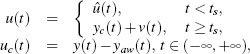
where û(t) is the plant input before the switch. This input may come from a manual control input or from the output of a different controller having authority over the plant input before the switch.

Figure 9.8 The bumpless transfer extension of the MRAW scheme.
The (–∞, +∞) specification in equations (9.12) denotes the fact that the scheme of Figure 9.8 should be implemented by interconnecting the controller to the plant output long before the switching time ts, so that the closed-loop transient induced by this interconnection will only happen virtually between the controller state xc and the anti-windup state xaw. In this way, the plant won't be affected by it. After the controller transient has expired, the switch can occur and bumpless transfer will be enforced by the stabilizing signal v, which had remained disconnected until that time.
Clearly, the length of this transient (therefore an estimate of how long the controller should be connected to the plant before the switching time ts) depends on the closed-loop system dynamics and on the nature of the disturbances affecting the closed loop. It might be in general a strong limitation to wait for the transient to expire before turning on the controller. To address this situation, denote by to the power-on time for the controller-filter pair represented by the two lower blocks in Figure 9.8. If the switching time ts is relatively close to the power-on time t0, the following two strategies can be useful to speed-up the transient controller response commented above:
1. The controller state at the initial time t0 may be initialized with a value which matches (in an averaged sense) the current plant state. Note that no requirement is imposed on this initial state, although a good guess may reduce the transient response.
2. In cases where the plant is operating around the steady state and the disturbances and the references have a sufficiently uniform frequency content (or are constant), the controller and filter dynamics may be run at a faster rate during the interval before the switching time ts. This strategy will accordingly speed up the controller transient and prepare the controller for the switch in a faster way. The correct timing of both controller and filter could then be reestablished gracefully just before the switching time ts.
Once the controller-anti-windup filter pair in Figure 9.8 have completed their transient, the control scheme may be switched on and off multiple times. After each switch on time, bumpless transfer will occur, based on the information stored into the state xaw of the AWBT filter. This feature may be useful in a multicontroller scheme where certain task oriented controllers are required to operate during some control phases. The bumpless transfer scheme would guarantee a smooth authority transfer among the different controllers. Notice, however, that the AWBT filter should be replicated for each controller involved in the multicontroller scheme. A block diagram illustrating this fact is represented in Figure 9.9. Another situation where this scheme might be useful is the case when certain controllers need to be tested in the feedback loop. In that case, a security transfer to a previously tested controller could be commanded at any time, guaranteeing the bumpless transfer feature.
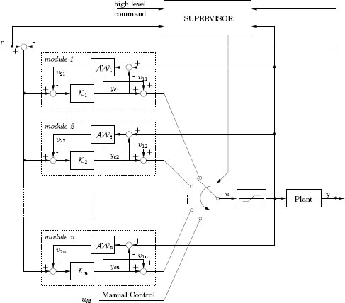
Figure 9.9 The bumpless transfer extension of the MRAW scheme in a multicontroller situation.
Finally, for the case where there is some flexibility in the switching time ts, an advantageous property of the model recovery AWBT solution is that the amount of transient to be experienced just after the switching phase is proportional to the size of the anti-windup filter state xaw. Indeed, because of the model recovery properties discussed in Section 6.3.2 on page 162 (see equation (6.14)), this state keeps track of the mismatch between the actual plant response and the target plant response that the controller would like to enforce on the plant. It is then reasonable to perform an “intelligent switch” by monitoring the size (e.g., the Euclidean norm) of xaw(·) to select the switching instant as an instant when this size is small, subject also to the constraint that t0 « ts. The corresponding performance output will almost instantaneously follow the target output response. Ideally, if t0 = – ∞ and one could find a time T where xe(T) = 0, then the switching transient would be completely removed by the bumpless transfer scheme. For an example, see the bold solid curve in the simulation results of Figure 9.10.
Example 9.3.1 (Bumpless plant startup) Consider a simple marginally stable SISO system characterized by an input saturation level of 0.25 and by the following state-space matrices:
![]()
and design two controllers. The first controller is an LQG controller which enforces a slow closed-loop behavior and is used at startup. The second controller is more aggressive and is designed with two internal models aimed at guaranteeing zero steady-state error for step references and at rejecting sinusoidal disturbances with unitary frequency (namely, the controller has three poles, at 0, + j, – j). To suitably stabilize the closed-loop system the second controller is completed by designing an LQG stabilizer for the plant augmented with the internal models.

Figure 9.10 Responses of the control authority transfer for Example 9.3.1.
Since the plant is marginally stable, MRAW can be designed for the system following Algorithm 11 for the synthesis of v. The resulting selection is v = –Kxaw with K = [0.002 -100]. Note that this scheme will work for any (even nonlinear) controller designed for this plant.
The simulation scenario is that of a plant startup where the first controller is used first and then authority is switched to the second controller to guarantee asymptotic reference tracking and disturbance rejection. The reference is a unit step and the disturbance is a sine wave of amplitude 0.2 affecting the plant input (namely, Bp,w = BP,U and Dp,yw = Dp,yu). Figure 9.10 represents three responses. The dotted line in the upper plot represents the reference signal. The dotted line in the lower plot corresponds to the input response that the second controller would have generated if it had been connected to the plant since t0 = –∞ This can be seen as the target response that the controller output should reach after the switching transient.
For the thin solid and dashed curves the switching time is fixed at ts = 15 and it is evident from the upper plot that the bumpless scheme rapidly drives the plant response to the reference value (note that the input authority is fully exploited by the scheme because in the lower plot, the plant input is kept into saturation until the transfer error becomes very small). The bold solid curve represents the results arising from applying the “intelligent switching” idea outlined above. In this case, the switching time is commanded upon detection of a very small Euclidean norm of the state xaw. In particular, slightly after time t = 14, this state is almost zero and the bumpless switch happens without any transient.![]()
9.4 RELIABLE CONTROL VIA HARDWARE REDUNDANCY
Following the discussion on bumpless transfer, a natural idea to consider is the possibility of assigning the n controllers in Figure 9.9 as multiple copies of the same controller. This may be desirable as a means for increasing the reliability of control schemes subject to actuator, sensor or other hardware failures.
When all of the controllers in Figure 9.9 reproduce the same dynamics, all of the controller outputs yci coincide at all times and switching among the different modules does not affect the system response. However, with the aim of increasing the reliability of the nominal control scheme, the multiple controller structure is a useful tool. In particular, if each controller has a dedicated sensor located on the plant for the measurement of the output y, then there are two main reasons for differences among the state responses xci of the controllers:
1. differences among measurement noise associated to each sensor;
2. controller failures, either corresponding to failures of the sensors or failures of the controlling device (a DSP board, a PLC or any other digital or analog device that implements the controller dynamics).
Due to the stability of the unconstrained closed-loop system and to the presence of an AWBT compensator for each controller, bounded measurement disturbances correspond to bounded differences among the controllers’ responses. On the other hand, if a failure occurs in the ith controller, typically the control objective is no longer met by the ith unconstrained closed-loop system, whose information is stored in the ith AWBT compensator. In this case, differences will eventually be observed between the input (or, similarly, the output) of the ith controller and the inputs (or, respectively, the outputs) of the other controllers. Based on these differences, the “supervisor” block in Figure 9.9 can be designed as a system detecting controller failures based on the measurement of the input-output pairs (uci, yci) i = 1,…, n. Upon a failure detection, the supervisor can switch off the defective controller and guarantee correct functioning of the overall control system.
Although the supervisor block can be implemented in many different ways, depending on the particular application, a possible general scheme is to define a maximum tolerance relating the differences among inputs and outputs of the controllers and, provided a majority of controllers are operating correctly, failures can be detected by comparing the responses (uci, yci). The responses corresponding to the majority of controllers that are operating correctly will differ by a small amount, while their difference with the malfunctioning ones will exceed the tolerance, thus allowing the failure to be detected.
A controller failure can occur in two main situations.
1. The failing controller is not connected to the plant. In this case, after the failure is detected, the controllercan be shut offand repaired without affecting the control performance. As a matter of fact, in Figure 9.9 it is clear that any disconnected controller is affected by the plant but does not affect the plant, because its output is disconnected. Once the controller is repaired, it can be reconnected to the reliable scheme and, after a transient (which, once again, does not affect the plant input), its state will converge to the values of the other controllers’ states thus reconstituting its normal operation. Note that the whole maintenance process for the controller is invisible to the plant.
2. The failing controller is connected to the plant. In this case, before the failure is detected, the state of the plant could be driven far from the desired trajectory. However, due to the bumpless scheme, once the control input is switched to a functioning controller, the state of the plant is driven back to the unconstrained trajectory (whose information is kept in the AWBT compensator of the new controller). Once the malfunctioning controller is disconnected from the plant input, it can be repaired and reconnected to the reliable scheme as described in the previous item.
In summary, the proposed reliable scheme guarantees the following properties:
• In addition to guaranteeing fault detection, the design also provides bumpless transfer between the malfunctioning controller and a functioning one.
• The proposed method is able to detect any fault occurring in the control loop: even when this corresponds to a slight malfunctioning that slowly drives the plant output far from the desired trajectory; as a matter of fact, the information about the desired trajectory is embedded in the reliable scheme and constantly compared to the plant response.
• Once the reliable design is implemented, the anti-windup property of the resulting controller with respect to possible plant input saturation is automatically guaranteed by the reliable scheme.
In the following example, the controller designed for the damped mass-spring system discussed in Example 7.2.6 on page 190 is replicated in a reliable scheme. Sensor failures are assumed in the system to demonstrate the abilities of the reliable scheme.
Example 9.4.1 (Reliable control for the damped mass-spring system) Consider the unconstrained control design for the damped mass-spring system of Example7.2.6 on page 190 and assume that three copies of that unconstrained controller are combined in a reliable scheme. Assume that the reference signal is a sawtoothed wave of period 5 seconds and amplitude 1.6 meters. Assume that the measurement of each sensor is affected by band-limited white noise with noise power 10-4.

Figure 9.11 Input and output of the plant in the reliable control scheme. The dashed vertical lines correspond to the sensor failures times.
Assume that the sensor of the first controller fails at time tF1 = 3 seconds giving a zero output from time tF1 until its repair time tR1 = 10 seconds. Assume also that the sensor of the second controller fails at time tF2 = 15.5 seconds, giving a large constant output value after that time.
Figure 9.11 represents the response of the system when the supervisor block only compares the various controller outputs yci, i = 1, 2, 3, with tolerance value 0.4. The dotted line represents the reference signal, the dashed-dotted line represents the unconstrained response (in the absence of measurement noise), and the solid line represents the response of the reliable control scheme. Sensor failures occur at the vertical dashed lines. The three controller outputs in the reliable scheme are shown in Figure 9.12, where solid lines are used when the controller is connected to the plant and dotted lines are used when the controller is disconnected from the plant.
At the system power-on, the first controller is active. In Figure 9.12 it is shown that the sensor failure at time tF 1 is detected with a significant delay and this causes the plant output to exhibit the bump in the top plot of Figure 9.11. Note that the sensor failure could be detected earlier by comparing the controller inputs uci, i = 1, 2, 3 in the supervisor block. However, it is of interest to show how the bumpless scheme is able to steer the plant output back to the desired trajectory even when the malfunctioning detection is delayed.

Figure 9.12 Outputs of the three redundant controllers in the reliable control scheme. Solid lines mean that the controller is connected to the plant. Controller repairs occur at the dashed-dotted vertical lines.
At time tR1, the first controller is repaired and reconnected to the plant output. After a short transient, it is again correctly functioning in the reliable scheme and it is used, together with the third controller, to detect the failure of the second sensor at time tF2 by majority comparison. After this second failure, it is assumed that the second sensor gives a large constant response, thus driving the malfunctioning controller output to large values (see the middle plot in Figure 9.12), hence the failure is detected almost instantly by the supervisor and no bump is noticeable on the plant output as seen in Figure 9.11. After the failure is detected, the plant input is switched to the third controller output until the end of the simulation.![]()
9.5 NOTES AND REFERENCES
The rate and magnitude saturation compensation scheme discussed here is taken from [AP2] where the scheme was applied to the example study discussed in Example 9.1.2. The study in [AP2] was motivated by the fact that previous papers [SAT4, SAT6] illustrated weaknesses of the daisy-chained scheme for redundant actuators in the presence of rate saturation. As in [AP2], the controller parameters are taken from [SAT4]. The Caltech ducted fan case study in Example 9.1.1 is taken from [AP3] where experimental results are also reported. The recent work in [MR33] provides additional algorithms for MRAW-based solutions of the anti-windup problem with rate- and magnitude-saturated plants. Those algorithms are not reported here to keep the discussion simple but might be included in a revised version of this book.
The MRAW solution for dead-time systems presented in Section 9.2 is taken from [MR24]. Example 9.2.1 is also taken from [MR24] but was originally presented in [G11, Example 4], where the unconstrained controller of Figure 9.5 was proposed. However, in [G11] the example was discussed in the absence of saturation.
The bumpless transfer extension of the MRAW scheme discussed in Section 9.3 is taken mainly from [MR25], where the corresponding theory is presented both in continuous and discrete time. The reader is also referred to [AP10], where a more sophisticated case study consisting in the dynamics of an open water channel has been studied, both in the discrete- and in the continuous-time setting. The multicontroller scheme of Figure 9.9 is taken from [MR15], which contains preliminary results on model recovery bumpless transfer and also contains the reliable control ideas of Section 9.4.