THE DECISION MAKING techniques we looked at in the last chapter have two important limitations: they are intended for use by a single character, and they don’t try to infer from the knowledge they have to a prediction of the whole situation.
Each of these limitations is broadly in the category of tactics and strategy. This chapter looks at techniques that provide a framework for tactical and strategic reasoning in characters. It includes methods to deduce the tactical situation from sketchy information, to use the tactical situation to make decisions, and to coordinate between multiple characters.
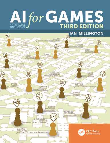
In the model of AI I’ve been using so far, this provides the third layer of our system, as shown in Figure 6.1.
It is worth remembering again that not all parts of the model are needed in every game. Tactical and strategic AI, in particular, is simply not needed in many game genres. Where players expect to see predictable behavior (in a two-dimensional [2D] shooter or a platform game, for example), it may simply frustrate them to face more complex behaviors.
There has been a rapid increase in the tactical capabilities of AI-controlled characters over the last ten years, partly because of the increase in AI budgets and processor speeds, and partly due to the adoption of simple techniques that can bring impressive results, as we’ll see in this chapter. It is an exciting and important area to be working in, and there is no sign of that changing.
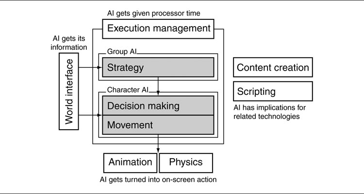
Figure 6.1: The AI model
A waypoint is a single position in the game level. We met waypoints in Chapter 4, although there they were called “nodes” or “representative points.” Pathfinding uses nodes as intermediate points along a route through the level. This was the original use of waypoints, and the techniques in this section grew naturally from extending the data needed for pathfinding to allow other kinds of decision making.
When we used waypoints in pathfinding, they represented nodes in the pathfinding graph, along with associated data the algorithm required: connections, quantization regions, costs, and so on. To use waypoints tactically, we need to add more data to the nodes, and the data we store will depend on what we are using the waypoints for.
In this section we’ll look at using waypoints to represent positions in the level with unusual tactical features, so a character occupying that position will take advantage of the tactical feature. Initially, we will consider waypoints that have their position and tactical information set by the game designer. Then, we will look at ways to deduce first the tactical information and then the position automatically.
Waypoints used to describe tactical locations are sometimes called “rally points.” One of their early uses in simulations (in particular military simulation) was to mark a fixed safe location that a character in a losing firefight could retreat to. The same principle is used in real-world military planning; when a platoon engages the enemy, it will have at least one pre-determined safe withdrawal point that it can retreat to if the tactical situation warrants it. In this way a lost battle doesn’t always lead to a rout.
More common in games is the use of tactical locations to represent defensive locations, or cover points. In a static area of the game, the designer will typically mark locations behind barrels or protruding walls as being good cover points. When a character engages the enemy, it will move to the nearest cover point in order to provide itself with some shelter.
There are other popular kinds of tactical locations. Sniper locations are particularly important in squad-based shooters. The level designer marks locations as being suitable for snipers, and then characters with long-range weapons can head there to find both cover and access to the enemy.
In stealth games, characters that also move secretly need to be given a set of locations where there are intense shadows. Their movement can then be controlled by moving between shadow regions, as long as enemy sight cones are diverted (implementing sensory perception is covered in Chapter 11, World Interfacing).
There are unlimited different ways to use waypoints to represent tactical information. We could mark fire points where a large arc of fire can be achieved, power-up points where power-ups are likely to respawn, reconnaissance points where a large area can be viewed easily, quick exit points where characters can hide with many escape options if they are found, and so on. Tactical points can even be locations to avoid, such as ambush hotspots, exposed areas, or sinking sand.
Depending on the type of game you are creating, there will be several kinds of tactics that your characters can follow. For each of these tactics, there are likely to be corresponding tactical locations in the game, either positive (locations that help the tactic) or negative (locations that hamper it).
A Set of Locations
Most games that use tactical locations don’t limit themselves to one type or another. The game level contains a large set of waypoints, each labeled with its tactical qualities. If the waypoints are also used for pathfinding, then they will also have pathfinding data such as connections and regions attached.
In practice, locations for cover and sniper fire are not very useful as part of a pathfinding graph. Figure 6.2 illustrates this situation. Although it is most common to combine the two sets of waypoints, it may provide more efficient pathfinding to have a separate pathfinding graph and tactical location set. You would have to do this, of course, if you were using a different method for representing the pathfinding graph, such as navigation meshes or a tile-based world.
We will assume for most of this section that the locations we are interested in are not necessarily part of the pathfinding graph. Later, we’ll see some situations in which merging the two together can provide very powerful behavior with almost no additional effort. In general, however, there is no reason to link the two techniques.

Figure 6.2: Tactical points are not the best pathfinding graph
Figure 6.2 shows a typical set of tactical locations for an area of a game level. It combines three types of tactical locations: cover points, shadow points, and sniping points. Some points have more than one tactical property. Most of the shadow points are also cover points, for example. There is only one tactical location at each of these locations, but it has both properties.
Marking all useful locations can produce a large number of waypoints in the level. To get very good quality behavior, this is necessary but time consuming for the level designer. Later in the section we’ll look at some methods of automatically generating the waypoint data.
Primitive and Compound Tactics
In most games, having a set of pre-defined tactical qualities (such as sniper, shadow, cover, etc.) is sufficient to support interesting and intelligent tactical behavior. The algorithms we’ll look at later in this section make decisions based on these fixed categories.
We can make the model more sophisticated, however. When we looked at sniper locations, I mentioned that a sniper location would have good cover and provide a wide view of the enemy. We can decompose this into two separate requirements: cover and view of the enemy. If we support both cover points and high visibility points in our game, we have no need to specify good sniper locations. We can simply say the sniper locations are those points that are both cover points and reconnaissance points. Sniper locations have a compound tactical quality; they are made up of two or more primitive tactics.

Figure 6.3: Ambush points derived from other locations
We don’t need to limit ourselves to a single location with both properties, either. When a character is on the offensive in a firefight, it needs to find a good cover point very near to a location that provides clear fire. The character can duck into the cover point to reload or when incoming fire is particularly dense and then pop out into the fire point to attack the enemy. We can specify that a defensive cover point is a cover point with a fire point very near (often within the radius of a sideways roll: the stereotypical animation for getting in and out of cover).
In the same way, if we are looking for good locations to mount an ambush, we could look for exposed locations with good hiding places nearby. The “good hiding places” are compound tactics in their own right, combining locations with good cover and shadow.
Figure 6.3 shows an example. In the corridor, cover points, shadow points, and exposed points are marked. We decide that a good ambush point is one with both cover and shadow, next to an exposed point. If the enemy moves into the exposed point, with a character in shadow, then it will be susceptible to attack. The good ambush points are marked in the figure.
We can take advantage of these compound tactics by storing only the primitive qualities. In the example above, we store three tactical qualities: cover, shadow, and exposure. From these we can calculate the best places to lay or avoid an ambush. By limiting the number of different tactical qualities, we can support a huge number of different tactics without making the level designer’s job impossible or flooding the memory with waypoint data that are rarely needed. On the other hand, what we gain in memory, we lose in speed. To work out the nearest ambush point, we would need to look for cover points in shadow and then check each nearby exposed point to make sure it was within the radius we were looking for.
In the vast majority of cases this extra processing isn’t important. If a character needs to find an ambush location, for example, then it is likely to be able to think for several frames. Decision making based on tactical locations isn’t something a character needs to do every frame, and so for a reasonable number of characters time isn’t of the essence.
For lots of characters or if the set of conditions is very complex, however, the waypoint sets can be pre-processed offline, and all the compound qualities can be identified. This doesn’t save memory when the game is running, but it removes the need for the level designer to specify all the qualities of every location. This can be taken further, and we can use algorithms to detect even the primitive qualities. I will return to algorithms for automatically detecting primitive qualities later in this section.
Waypoint Graphs and Topological Analysis
The waypoints I have described so far are separate, isolated locations. There is no information as to whether one waypoint can be reached from another. I mentioned at the start of this section the similarity of waypoints to nodes in a pathfinding graph. We can certainly use nodes in a pathfinding graph as tactical locations (although they aren’t always the best suited, as we’ll see later in Section 6.3 on tactical pathfinding).
But even if we aren’t using a pathfinding graph, we can link together tactical locations to give access to more sophisticated compound tactics.
Let’s suppose that we’re looking for somewhere that provides a good location to mount a hit and run attack. The set of waypoints in Figure 6.4 shows part of a level to consider. Waypoints are connected when one can be reached from the other directly. There are no connections through the wall, for example. In the balcony we have a location (A) with good visibility of the room, a candidate for an attack spot. Similarly, there is one other location in a small anteroom (B) that might be useful.
The balcony is obviously better than the anteroom because it has three exits, only one of which leads into the room. If we are looking to perform a hit and run attack, then we need to find locations with good visibility, but lots of exit routes.
This is a topological analysis. It reasons about the structure of the level by looking at the properties of the waypoint graph. It is a kind of compound tactic, but one that uses the connections between waypoints as well as their tactical qualities and positions.
Topological analysis can be performed using the pathfinding graph, or it can be performed on basic tactical waypoints. It does require connections between waypoints, however. Without these connections, we wouldn’t know whether the nearby waypoints constitute exit routes or whether there was a wall between them.
Unfortunately, this kind of topological analysis can rapidly get complicated. It is extremely sensitive to the density of waypoints. Take location C in Figure 6.4. Once again the shooting position has three exit routes. In this case, however, they all lead to locations in the same vicinity with immediate escape. The character looking for a good hit and run location based on the number of exits alone might mistakenly mount its attack in the middle of the room.
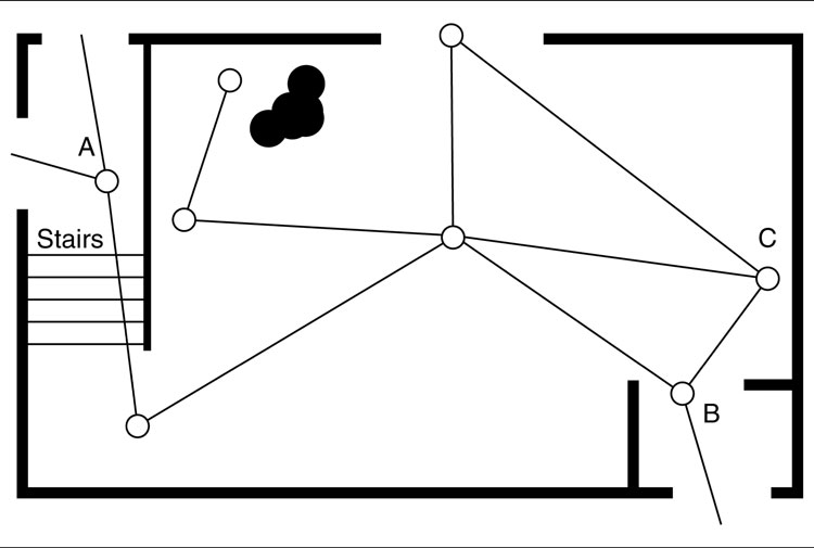
Figure 6.4: Topological analysis of a waypoint graph
Of course, we can make the topological analysis algorithm more sophisticated. We could look not just at the number of connections, but also where those connections lead, and so on.
In my experience the complexity of this kind of analysis is formidable and beyond what most developers want to spend time implementing and tweaking. In my opinion, there isn’t much debate between developing a comprehensive topological analysis system and having a level designer simply specify the appropriate tactical locations. For all but the simplest analysis, the level designer gets the job every time.
Automatic topological analysis comes up from time to time in books and papers. My advice would be to treat it with caution, unless you can spare a couple of months of playing to get it right. The manual way is often less painful in the long run.
Continuous Tactics
To support more complicated compound tactics, we can move away from simple Boolean states. Rather than marking a location as being “cover” or “shadow,” for example, we can provide a numerical value for each. A waypoint will have a value for “cover” and a different value for “shadow.”
The meaning of these values will depend on the game, and they can have any range that is convenient. For the purpose of clarity, however, let’s assume the values are floating points in the range (0, 1), where a value of 1 indicates that the waypoint has the maximum amount of a property (a maximum amount of cover or shadow, for example).
On its own we can use this information to simply compare the quality of a waypoint. If a character is trying to find cover, and it has equally achievable options between a waypoint with cover = 0.9 or cover = 0.6, it should head for the waypoint with cover = 0.9.
We can also interpret these values as a degree of membership of a fuzzy set (the basics of fuzzy logic were described in Chapter 5, Decision Making). A waypoint with a “cover” value of 0.9 has a high degree of membership in the set of cover locations.
Interpreting the values as degrees of membership allows us to produce values for compound tactics using the fuzzy logic rule. Recall that we defined a sniper location as a waypoint that had both a view of the enemy and good cover. In other words,
![]()
If we have a waypoint with cover = 0.9 and visibility = 0.7, we can use the fuzzy rule:
where mA and mB are the degrees of membership of A and B. Adding in our data we get:
So we can derive the quality of a sniper location and use that as the basis of a character’s tactical actions. This example is very simple, using just AND to combine its components. As we saw in the previous section, we can devise considerably more complex conditions for compound tactics. Interpreting the values as degrees of membership in fuzzy states allows us to work with even the most complex definitions made up of lots of clauses. It provides a tried and tested mechanism for ending up with a dependable value.
The disadvantage of using this approach is that each waypoint needs to have a complete set of values stored for it. If we are keeping track of five different tactical properties, then for the non-numeric situation we only need to keep a list of waypoints in each set. There is no wasted storage. On the other hand, if we store a numeric value for each, then there will be five numbers for each waypoint.
We can slightly reduce the need for storage by not storing zero values, although this makes things more complex because we need a reliable way to store both the value and the meaning of that value (if we always store the five numbers, then we can tell what each number means by its position in the array).
For large outdoor worlds, such as those used in real-time strategy (RTS) or massively multiplayer games, we might be driven to save memory. In most shooters, however, the extra memory is unlikely to cause problems.
Context Sensitivity
However, there is still a problem with marking tactical locations in the way I’ve described so far. The tactical properties of a location are almost always sensitive to actions of the character or the current state of the game.
Hiding behind a barrel, for example, might produce cover only if the character is crouched. If the character stands behind the barrel, it is a sitting duck for incoming fire. Likewise, hiding behind a protruding rock is of no use if the enemy is behind you. The aim is to put the rock between the character and the incoming fire.
This problem isn’t limited to just cover points. Any of the tactical locations in this section may be invalid in certain circumstances. If the enemy manages to mount a flank attack, then there is no use heading for a withdrawal location which is now behind enemy lines.
Some tactical locations have an even more complicated context. A sniper point is likely to be useless if everyone knows the sniper is camped there. Unless it happens to be an impenetrable hideout (which is a sign of faulty level design, I would suggest), then sniper positions depend to some extent on secrecy.
There are two options for implementing context sensitivity. First, we could store multiple values for each node. A cover waypoint, for example, might have four different directions. For any given cover point, only some of those directions are covered. These four directions are the states of the waypoint. For cover, we have four states, and each of these may have a completely independent value for the quality of the cover (or just a different yes/no value if we aren’t using continuous tactic values). We could use any number of different states. We might have an additional state that dictates whether the character needs to be ducking to receive cover, for example, or additional states for different enemy weapons; a location that provides cover from small arms fire might not protect its inhabitant from an RPG.
For tactics where the set of states is fairly obvious, such as cover or firing points (we can use the four directions again as firing arcs), this is a good solution. For other types of context sensitivities, it is more difficult. In our example of the withdrawal location, it is not obvious how to specify a sensible set of different states for the territory controlled by the enemy.
The second approach is to use only one state per waypoint, as we have seen throughout this section. Rather than treating this value as the final truth about the tactical quality of a waypoint, we add an extra step to check if it is appropriate. This checking step can consist of any check against the game state. In the cover example we might check for line of sight with our enemies. In the withdrawal example we might check on an influence map (see Section 6.2.2 on influence mapping later in this chapter) to see if the location is currently under enemy control.
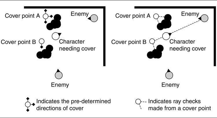
Figure 6.5: A character selecting a cover point in two different ways
In the sniper example we could simply keep a list of Boolean flags to track if the enemy has fired toward a sniper location (a simple heuristic to approximate if the enemy knows the location is there). This post-processing step has similarities to the processing used to automatically generate the tactical properties of a waypoint. I will return to these techniques later.
As an example of each approach, consider a character that needs to choose a cover point to reload behind during a firefight. There are two cover points nearby that it can select from, as shown in Figure 6.5.
In the diagram on the left of Figure 6.5 the cover points are shown with their quality of cover in each of the four directions. The character works out the direction to each enemy and determines that it needs cover from the south and east directions. So the character checks for a cover point that provides that. Cover point B does, and it selects that point.
In the diagram on the right of Figure 6.5 a runtime check has been used. The character checks the line of sight from both cover points to both enemies. It determines that cover point B does not have a line of sight to either, so it is preferable to cover point A that has a line of sight to one enemy.
The trade-off between these two methods is between quality, memory, and execution speed. Using multiple states per waypoint makes decision making fast. We don’t need to perform any tactical calculations during the game. We just need to work out which states we are interested in. On the other hand, to get very high-quality tactics we may need a huge number of states. If we need cover in four directions, both standing and crouched, against any of five different types of weapons, we’d need 40 states for a cover waypoint. Clearly, this can very quickly become too much.
Performing a runtime check gives us much more flexibility. It allows the character to take advantage of quirks in the environment. A cover point may not provide cover to the north except for attacks from a particular walkway (the position of a roof girder provides cover there, for example). If the enemy is on that walkway, then the cover point is valid. Using a simple state for the cover from northerly attacks would not allow the character to take advantage of this.
On the other hand, runtime checking takes time, especially if we are doing lots of line-of-sight checks through the level geometry. In tactically complicated games, line-of-sight checks may take up the majority of all the AI time used in the game: over 30% of the total processor time in one case I’m familiar with. If you have a lot of characters that have to react quickly to changing tactical situations, this may be unacceptable. If the characters can afford to take a couple of seconds to weigh up their options, then you can split these checks over multiple frames and it is unlikely to be a problem.
In my opinion, only games aimed at hard-core players that really benefit from good tactical play, such as squad-based shooters, need the runtime checking approach. For other games where tactics aren’t the focus, a small number of states will be sufficient. It is possible to combine both approaches in the same game, with the multiple states providing a filtering mechanism that reduce the number of different cover waypoints requiring line-of-sight checks.
Putting It Together
We’ve considered a range of complexities for tactical waypoints, from a simple label for the tactical quality of a location through to compound, context-sensitive tactics based on fuzzy logic. In practice, most games don’t need to go the whole way.
Many games can get away with simple tactical labels. If this produces odd behavior, then the next stage to implement is context sensitivity, which provides a huge increase in the competency of the AI.
Next, I suggest adding continuous tactical values and allow characters to make decisions based on the quality of a waypoint.
For highly tactical games where the quality of the tactical play is a selling point for the game, using compound tactics (with fuzzy logic) then allows you to support new tactics without adding or changing the information that the level designer needs to create. So far I haven’t worked on a game that has gone this far, although it isn’t new in the field of military simulation.
6.1.2 USING TACTICAL LOCATIONS
So far we’ve looked at how a game level can be augmented with tactical waypoints. However, on their own they are just values. We need some mechanism to include their data into decision making.
We’ll look at three approaches. The first is a very simple process for controlling tactical movement. The second incorporates tactical information into the decision making process. The third uses tactical information during pathfinding to produce character motion that is always tactically aware. None of these three approaches is a new algorithm or technique. They are simply ways in which to bring the tactical information into the algorithms we looked at in previous chapters.
For now, our focus will be limited to decision making for a single character. Later, in Section 6.4, I will return to the task of coordinating the actions of several characters, while making sure they remain tactically aware.
Simple Tactical Movement
In most cases a character’s decision making process implies what kind of tactical location it needs. For example, we might have a decision tree that looks at the current state of the character, its health and ammo supply, and the current position of the enemy. The decision tree is run, and the character decides that it needs to reload its weapon.
The action generated by the decision making system is “reload.” This could be achieved simply by playing the reload animation and updating the number of rounds in the character’s weapon. Alternatively, and more tactically, we can choose to find a suitable place to reload, under cover.
This is simply achieved by querying the tactical waypoints in the immediate vicinity. Suitable waypoints (in our case, waypoints providing cover) are found, and any post-processing steps are taken to ensure that they are suitable for the current context.
The character then chooses a suitable location and uses it as the target of its movement. The choice can be simply “the nearest suitable location,” in which case the character can begin with the nearest waypoint and check them in order of increasing distance until a match is found. Alternatively, we can use some kind of numeric measure of how good a location is. If we are using continuous values for the quality of a waypoint, this might be what we need. We are not necessarily interested in selecting the best node in the whole level, however. There is no point in running all the way across the map just to find a really secure location to reload. Instead, we need to balance distance and quality.
This approach makes the action decision first, independent of the tactical information, and then applies tactical information to achieve its decision. It is a powerful technique on its own and forms the basis of most squad-based AI. It is the bread and butter of shooters right through to present titles.
It does have a significant limitation, however. Because the tactical information isn’t used in the decision making process, we may end up discovering the decision is foolish only after the decision has been made. We might find, for example, that after making a decision to reload, we can’t find anywhere safe nearby to do so. A person in this situation would try something different. For example, they may choose to run away. If the character is committed to the decision, however, it will be stuck and appear foolish.
Games rarely allow the AI to detect this and go back and reconsider the decision.
In most games this isn’t a significant problem in practice, particularly if the level designer is clued up. Every area in the game usually has several tactical points of each type (with the exception of sniping points, perhaps, but we normally don’t mind if characters go wandering off a long way to find these).
When it is an issue, however, we need to take account of the tactical information in the original decision making process.
Using Tactical Information Like Any Other Data
The simplest way to bring tactical information into the decision making process is to give the decision maker access to it in the same way as it has access to other information about the game world.
If we want to use a decision tree, for example, we could allow decisions to be made based on the tactical context of the character. We might make a decision based on the nearest cover point, as Figure 6.6 shows. The character in this case will not decide to head for cover and then find there is no suitable cover. The decision to move to cover takes into account the availability of cover points to move to.
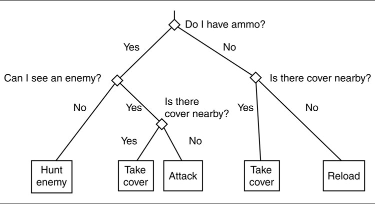
Figure 6.6: Tactical information in a decision tree
Similarly, if we are using a state machine we might only trigger certain transitions based on the availability of waypoints.
In both of these cases the code should keep track of any suitable waypoints it finds during decision making so that it can use them after the decision has been made. If the decision tree in the first example ends up suggesting the “take cover” action, then it will need to work out which cover point to take cover in.
This involves the same search for nearby decision points that we had using the simple tactical movement approach previously. To avoid a duplication of effort, we cache the cover point that is found during the decision tree processing. We then use that target in the movement AI and move directly toward it without further search.
Tactical Information in Fuzzy Logic Decision Making
For both decision trees and state machines, we can use tactical information as a yes or no condition, either at a decision node in the decision tree or as a condition of making a state transition.
In both cases we are interested in finding a tactical location where some condition is met (it might be to find a tactical location where the character can take cover, for example). We aren’t interested in the quality of the tactical location.
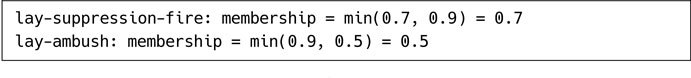
We can go one stage further and allow the decision making to take account of the quality of a tactical location as it makes a decision. Imagine a character is weighing up two strategies. It might camp out behind cover and provide suppression fire, or it might take up a position in shadow ready to lay an ambush to unwary enemies passing by. We are using continuous tactical data for each location, and the cover quality is 0.7 while the shadow quality is 0.9.
Using a decision tree, we would simply check if there is a cover point, and upon finding that there is, the character would follow the suppression fire strategy. There is no sense in weighing up the pros and cons of each option.
If we use a fuzzy decision making system, however, we can use the quality values directly in the decision making process. Recall from Chapter 5 that a fuzzy decision making system has a set of fuzzy rules. These rules combine the degrees of membership of several fuzzy sets into values that indicate which action is preferred.
We can incorporate our tactical values directly into this method, as another degree of membership value.
For example, we might have the following rules:

For the tactical values given above, we get the following result:

If the two values are independent (i.e., if it is impossible to do both at once, which we’ll assume it is), then we choose lay-ambush as the action to take.
The rules can be significantly more complex, however:

Now if we have the memberships values:

we would end up with the results:
and the correct action is to lay suppression fire.
There are no doubt numerous other ways to include the tactical values into a decision making process. We can use them to calculate priorities for rules in a rule-based system, or we can include them in the input state for a learning algorithm. This approach, using the rule-based fuzzy logic system, provides a simple to implement extension that gives very powerful results. It is not a well-used technique, however. Most games rely on a much simpler use of tactical information in decision making.
Generating Nearby Waypoints
If we use any of these approaches, we will need a fast method of generating nearby way-points. Given the location of a character, we ideally need a list of suitable waypoints in order of distance.
Most game engines provide a mechanism to rapidly work out what objects are nearby. Spatial data structures such as quad-trees or binary space partitions (BSPs) are often used for collision detection. Other spatial data structures such as multi-resolution maps (a tile-based approach with a hierarchy of different tile sizes) are also suitable. For tile-based worlds, we have also used stored patterns of tiles for different radii, simply superimposed the pattern on the character’s tile, and looked up the tiles within that pattern for suitable waypoints.
As I said in Chapter 3, spatial data structures for proximity and collision detection are beyond the scope of this book. There is another book in this series [14] that covers the topic. The references appendix lists this and other suitable resources.
Distance isn’t the only thing to take into account, however. Figure 6.7 shows a character in a corridor. The nearest waypoint is in an adjacent room and is completely impractical as a cover point. If we simply selected the cover point based on distance, we’d see the character run into a different room to reload, rather than use the crate near the end of the corridor.
We can minimize this problem with careful level design. It is often a sensible idea not to use thin walls in a game level. As we saw in Chapter 4, this can also confuse the quantization algorithm. Sometimes, however, it is unavoidable, and a better solution is required.
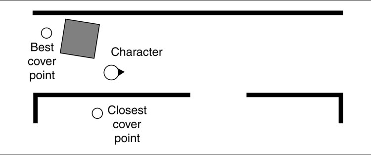
Figure 6.7: Distance problems with cover selection
Another approach would be to determine how close each tactical waypoint is by performing a pathfinding step to generate the distance. This then takes into account the structure of the level, rather than using a simple Euclidean distance. We can interrupt the pathfinding when we realize that it will be a longer path than the path to the nearest waypoint we’ve found so far. Even with such optimizations, this adds a significant amount of processing overhead.
Fortunately, we can perform the pathfinding and the search for the nearest target in one step. This also solves the problem of confusion by thin walls and of finding nearby waypoints. It also has an additional benefit: the route it returns can be used to make characters move, while constantly taking into account their tactical situation.
Tactical Pathfinding
Tactical waypoints can also be used for tactical pathfinding. Tactical pathfinding is a hot topic in game AI, but is a relatively simple extension of the basic A* pathfinding algorithm. Rather than finding the shortest or quickest route, however, it takes into account the tactical situation of the game.
Tactical pathfinding is more commonly associated with tactical analyses, however, so I’ll return to a full discussion in Section 6.3 later in the chapter.
6.1.3 GENERATING THE TACTICAL PROPERTIES OF A WAYPOINT
So far I have assumed that all the waypoints for our game have been created, and each has been given its appropriate properties: a set of labels for the tactical features of its location and possibly additional data for the quality of the tactical location, or context-sensitive information.
In the simplest case these are often created by the level designer. The level designer can place cover points, shadow points, locations with high visibility, and excellent sniper locations. As long as there are only a few hundred cover points, this task isn’t onerous. It is the approach used in a large number of shooters. Beyond the simplest games, however, the effort may increase dramatically.
If the level designer has to place context-sensitive information or set the tactical quality of a location, then the job becomes very difficult, and the tools needed to support the designer have to be significantly more complicated. For context-sensitive, continuous valued tactical waypoints, we may need to set up different context states and be able to enter numeric values for each. To make sure the values are sensible, we will need some kind of visualization.
While it is possible for the designer to place the waypoints, all the extra burden makes it unlikely that the level designer will be tasked with setting the tactical information unless it is of the simplest Boolean kind.
For other games we may not need to have the locations placed manually; they may arise naturally from the structure of the game. If the game relies on a tile-based grid, for example, then locations in the game are often positioned at corresponding tiles. While we know where the locations are, we don’t know the tactical properties of each one. If the game level is built up from prefabricated sections, then we could have tactical locations placed in the prefabs.
In both cases we need some mechanism for calculating the tactical properties of each waypoint automatically.
This is usually performed using an offline pre-processing step, although it can also be performed as it is needed during the game. The latter approach allows us to generate the tactical properties of a waypoint in the current game context, which in turn can support more subtle tactical behavior. As described in the section on context sensitivity above, however, this has a significant impact on performance, especially if there are a large number of waypoints to consider.
The algorithm for calculating a tactical quality depends on the type of tactic we are interested in. There are as many calculations as there are types of tactics. We will look at the types of waypoints we’ve used so far in the chapter to give a feel for the types of processing involved. Other tactics will tend to be similar to these types, but may need some modification.
Cover Points
The quality of a cover point is calculated by testing how many different incoming attacks might succeed. We run many different simulated attacks and see how many get through.
We can run a complete simulated attack, but this takes time. It is normally easier to approximate an attack by a line-of-sight test: a ray cast through the level geometry.
For each attack we start by selecting a location in the vicinity of the candidate cover point. This location will usually be in the same or an adjoining room to the cover point. We can test from everywhere in the level, of course, but that is wasteful as most attacks will not succeed. In outdoor levels we may have to check everywhere within weapons range, which is potentially a time-consuming process.
One way to do this is to check attacks at regular angles around the point. We need to first make sure that the location we are checking is in the same room or area as the point it is trying to attack. A point in the middle of a corridor, for example, can be hit from anywhere in the corridor. If the corridor is thin, however, using all the angles around will give a high cover value: most of the angles are covered by the corridor walls. Testing nearby locations that can be occupied, however, will show correctly that the point is 100% exposed.
Being too regular, however, can also lead to problems. If we test just locations around the point at the same height as the point, we might get the wrong value. A character standing behind an oil can, for example, can be covered from the ground level, but would be exposed from a gun at shoulder height. We can solve this problem by checking each angle several times, with small random offsets, and at different heights.
From the location we select, a ray is cast toward the candidate cover point. Crucially, the ray is cast toward a random point in a person-sized volume at the candidate point. If we aim toward just the point, we may be checking if a small point on the floor is covered, rather than the area a character would occupy.
This process is repeated many times from different locations. We keep track of the proportion of rays that hit the volume.
The pseudo-code to perform these checks looks like the following:
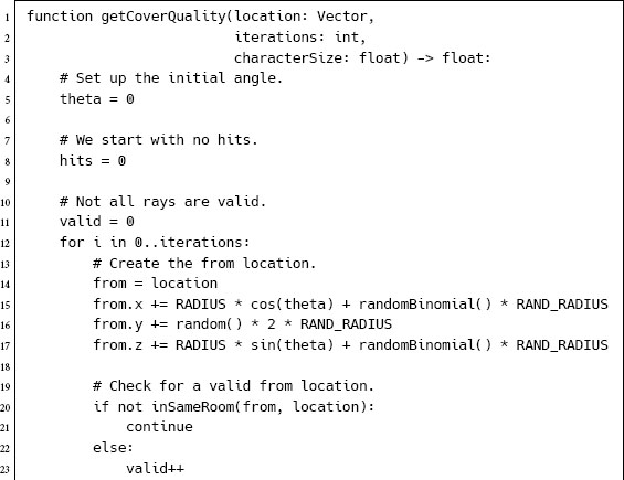

In this code, we have used a doesRayCollide function to perform the actual ray cast. rand returns a random number from 0 to 1, and randomBinomial creates a binomially distributed random number from –1 to 1, as before. inSameRoom checks if two locations are in the same room. This can be done very easily with a hierarchical pathfinding graph, for example, or can be calculated using a pathfinder.
There are a number of constants in the function. The RADIUS constant controls how far from the point to begin the attack. This should be far enough so that the attack isn’t trivially easy, but not so far that the attack is guaranteed to be in another room. It depends on the scale of your level geometry. The RAND_RADIUS constant controls how much randomness is added to the from location. This should be smaller than RADIUS sin ANGLE; otherwise, we will be moving it farther than it will move to check the next angle, and we’ll not cover all the angles correctly. The ANGLE constant controls how many samples around the point are considered. It should be set so that each angle is considered many times (i.e., the smaller the number of iterations, the larger ANGLE should be).
Context-sensitive values can be calculated in the same way as above. Rather than lumping all the results together, we need to calculate the proportion of ray casts that hit coming from each direction or the proportion that hit a crouched or standing character volume, depending on the contexts we are interested in.
If we are running the processing during the game, then there is no reason to choose random directions to test. Instead, we use the enemy characters that the AI is trying to find cover from to check the possibility of hitting the cover point. It is still a good idea to repeat the test several times with different random offsets, however. If time is a critical issue, we can skip this and only check a direct line of sight. This makes the algorithm faster, but it can be foiled by thin structures that happen to block the only ray tested.

Figure 6.8: Good cover and visibility
Visibility Points
Visibility points are calculated in a similar way to cover points, using many line of sight tests. For each ray cast, we select a location in the vicinity of the cover point. This time we shoot rays out from the waypoint (actually from the position of the character’s eyes if it was occupying the waypoint). There is no random component needed around the waypoint. We can use their eye location directly.
The quality of visibility for the waypoint is related to the average length of the rays sent out (i.e., the distance they travel before they hit an object). Because the rays are being shot out, we are approximating the volume of the level that can be seen from the waypoint: a measure of how good the location is for viewing or targeting enemies.
Context-sensitive values can be generated in the same way by grouping the ray tests into a number of different states.
At first glance it might seem like visibility and cover are merely opposites. If a location is a good cover point, then it is a poor visibility point. Because of the way the ray tests are performed, this isn’t the case. Figure 6.8 shows a point which has both good cover and reasonable visibility. It’s the same logic that has people spying through keyholes: they can see a good amount while maintaining low visibility themselves.
Shadow Points
Shadow points need to be calculated based on the lighting model for a level. Most studios now use some kind of global illumination (radiosity) lighting as a pre-processing step to calculate light maps for in-game use. For titles that involve a great deal of stealth, a dynamic shadow model is used at runtime to render cast shadows from static and moving lights.
To determine the quality of a shadow point, several samples are taken from a charactersized volume around the waypoint. For each sample, the amount of light at the point is tested. This might involve ray casts to nearby light sources to determine if the point is in shadow, or it may involve looking up data from the global illumination model to check the strength of indirect illumination.
Because the aim of a shadow point is to conceal, we take the maximum lightness found in the sampling. If we took the average, then the character would prefer a spot where its body was in very dark shadow but its head was in direct light, over a location where all its body was in moderate shadow. The quality of a hiding position is related to the visibility of the most visible part of the character, not its average visibility as a whole.
For games with dynamic lighting, the shadow calculations need to be performed at runtime. Global illumination is a very slow process, however, and is best performed offline. Combining the two can be problematic. Only in the last five years have developers succeeded in getting simple global illumination models running at interactive frame rates. This uses a form of ray tracing, and while there is interest in using ray tracing more generally as the core rendering mechanism, it is still largely experimental. Even if the experiments successful, we are some years away from that being the state-of-the-art.
Fortunately, in many current-generation games, no global illumination is used at runtime. The environments are simply lit by direct light, and the global illumination is handled with static texture maps. In this case the shadow calculations can be performed over several frames without a severe slowdown.
Compound Tactics
As described earlier, a compound tactic is one that can be assessed by combining a set of primitive tactics. A sniper location might be one that has both cover and good visibility of the level.
If compound tactics are needed in the game, we may be able to generate them as part of a pre-processing step, using the output results of the primitive calculations above. The results can then be stored as an additional channel of tactical information for appropriate waypoints. This only works if the tactics they are using are also available at this time. You can’t pre-process a compound tactic based on information that changes during the game.
Alternatively, we can calculate the compound tactical information dynamically during the game by combining the tactical data of nearby waypoints on the fly.
Generating Tactical Properties and Tactical Analysis
Generating the tactical properties of waypoints in this way brings us very close to tactical analysis, a technique I will return to in the next section. Tactical analysis works in a similar way: we try to find the tactical and strategic properties of regions in a game level by combining different concerns together.
Taking tactical waypoints to the extreme, using automatic identification of the tactical properties of a location, would be akin to performing a tactical analysis on a game level. Tactical analysis tends to use larger scale properties—for example, balance of power or influence—rather than the amount of cover.
It is not common to recognize the similarity, however. As fairly new techniques in game AI, they both tend to have their own devotees and advocates. It is worth recognizing the similarity and even combining the best of both approaches, as required by your game design.
6.1.4 AUTOMATICALLY GENERATING THE WAYPOINTS
In most games waypoints are specified by the level designer. Cover points, areas that are prone to ambush, and dark corners are all more easily identified by a human being than by an algorithm.
Some developers have experimented with the automatic placement of waypoints. The most promising approaches I have seen are similar to those used in automatically marking up a level for pathfinding.
Watching Human Players
If your game engine supports it, keeping records of the way human players act can provide good information on tactically significant locations. The position of each character is stored at each frame or every few frames. If the character remains in roughly the same location for several samples in a row, or if the same location is used by several characters repeatedly over the course of the game, then it is likely that the location is significant tactically.
With a set of candidate positions, we can then assess their tactical qualities, using the algorithms to assess the tactical quality we saw in the previous section. Locations with sufficient quality are retained as the waypoints to be stored for use in the AI.
It is worth generating far more candidate locations than you will end up using. The assessment of the tactical quality can then filter out the best waypoints from the rest. You do need to be careful in choosing just the best 50 waypoints, for example, because they may be concentrated in one part of the level, leaving no tactical locations in more tactically tight areas (where, conversely, they are probably more important).
A better approach is to make sure the best few locations for each type of tactic in a specific area are kept. This can be achieved using the condensation algorithm (see Section 6.1.5), a technique that can also be used on its own without generating the candidate locations by watching human players.
Condensing a Waypoint Grid
Rather than trying to anticipate the best locations in the game level, we can instead test (almost) every possible location in the level and choose the best.
This is usually done by applying a dense grid to all floor areas in the level and testing each one. First, the locations are tested to make sure they are a valid location for the character to occupy. Locations too close to the walls or underneath obstacles are discarded.
Valid locations are then assessed for tactical qualities in the same way as we saw in the previous section. In order to perform the condensation step, we need to work with real-valued tactical qualities. A simple Boolean value will not suffice.
Normally, we keep a set of threshold values for each tactical property. If a location doesn’t make the grade for any property, then it can be immediately discarded. This makes the condensation step much faster.
The threshold levels should be low enough so that many more locations pass than could possibly be needed. This is to avoid discarding locations that are significant, but only marginally. In a room where there is virtually no cover, a location with even very poor cover might be the best place to defend from.
The remaining locations then enter into a condensation algorithm, which ends with only a small number of significant locations in each area of the level for each tactical property. If we used the “watching player actions” technique above, then the tactical locations that resulted could be condensed in the same way as the remaining locations from a grid. Because it is useful in several contexts, it is worth taking a look at the condensation algorithm in more detail.
6.1.5 THE CONDENSATION ALGORITHM
The condensation algorithm works by having tactical locations compete against one another for inclusion into the final set. We would like to keep locations that are either very high quality or a long distance from any other waypoint of the same type.
For each pair of locations, we first check that a character can move between the locations easily. This is almost always done using a line-of-sight test, although it would be better to allow slight deviations. If the movement check fails, then the locations can’t compete with one another. Including this check makes sure that we don’t remove a waypoint on one side of a wall, for example, because there is a better location on the other side.
If the movement check succeeds, then the quality values for each location are compared. If the difference between the values is greater than a weighted distance between the locations, then the location with the lower value is discarded. There are no hard and fast rules for the weight value to use. It depends on the size of the level, the complexity of the level geometry, and the scale and distribution of quality values for the tactical property. The weight should be selected so that it gives the right number of output waypoints, and that means tweaking by hand so that it looks right. If you use a lower weight value, the difference in quality will be more important, leaving fewer waypoints. Higher weights similarly produce more waypoints.

Figure 6.9: Order dependence in condensation checks
If there are a large number of waypoints, then there will be a huge number of pairs to consider. Because the final check depends on distance, we can speed this up significantly by only considering pairs of locations that are fairly close together. If we are using a grid representation, this is fairly simple; otherwise, we may have to rely on some other spatial data structure to provide sensible pairs to test.
This condensation algorithm is highly dependent on the order in which pairs of locations are considered. Figure 6.9 shows three locations. If we perform a competition between locations A and B, then A is discarded. B is then checked against C. In this case C wins. We end up with only location C. If we first check B and C, however, then C wins. A is now too far from C for C to beat it, so both C and A remain.
To avoid removing a series of waypoints in this way, we start with the strongest waypoints and work down to the weakest. For each of these waypoints, we perform the competition against other waypoints working from the weakest to the strongest. The first waypoint check, therefore, is between the strongest and the weakest. Because we will only consider pairs of waypoints fairly close to one another, the first check is likely to be between the overall strongest waypoint and the weakest nearby waypoint.
The condensation phase should be carried out for each different tactical property. There is no use discarding a cover point because there is a good nearby ambush location, for example. The tactical locations that make it through the algorithm are those that are left in any property after condensation.
Pseudo-Code
The algorithm can be implemented in the following way:

Data Structures and Interfaces
The algorithm assumes we can get position and value from the waypoints. They should have the following structure:

The waypoints are presented in a data structure in a way that allows the algorithm to extract the elements in sequence and to perform a spatial query to get the nearby waypoints to any given waypoint. The order of elements is set by a call to either sort or sortReversed, which orders the elements either by increasing or decreasing value, respectively. The interface looks like the following:

The Trade-Off
Watching player actions produces better quality tactical waypoints than simply condensing a grid. On the other hand, it requires additional infrastructure to capture player actions and a lot of playing time by testers. To get a similar quality using condensation, we need to start with an exceptionally dense grid (in the order of every 10 centimeters of game space for average human-sized characters). This also has time implications. For a reasonably sized level, there could be billions of candidate locations to check. This can take many minutes or hours, depending on the complexity of the tactical assessment algorithms being used.
The results from these algorithms are less robust than the automatic generation of pathfinding meshes (which have been used without human supervision), because the tactical properties of a location apply to such a small area. Automatic generation of waypoints involves generating locations and testing them for tactical properties. If the generated location is even slightly out, its tactical properties can be very different. A location slightly to the side of a pillar, for example, has no cover, whereas it might provide perfect cover if it were immediately behind the pillar.
When graphs for pathfinding are automatically generated, however, the same kind of small error rarely makes any difference.
Because of this, I am not aware of anyone reliably using automatic tactical waypoint generation without some degree of human supervision. Automatic algorithms can provide a useful initial guess at tactical locations, but you will probably need to add facilities into your level design tool to allow the locations to be tweaked by the level designer.
Before you embark on implementing an automatic system, make sure you work out whether the implementation effort will be worth it for time saved in level design. If you are designing huge, tactically complex levels, it may be so. If there will only be a few tens of waypoints of each kind in a level, then it is probably better to go the manual route.
Tactical analyses of all kinds are sometimes known as influence maps. Influence mapping is a technique pioneered and widely applied in real-time strategy games, where the AI keeps track of the areas of military influence for both sides. Similar techniques have also made inroads into squad-based shooters and massively multi-player games. For this chapter, I will refer to the general approach as tactical analysis to emphasize that military influence is only one thing we might base our tactics on.
In military simulation an almost identical approach is commonly called terrain analysis (a phrase also used in game AI), although again that also more properly refers to just one type of tactical analysis. I will describe both influence mapping and terrain analysis in this section, as well as general tactical analysis architectures.
There is not much difference between tactical waypoint approaches and tactical analyses. By and large, papers and talks on AI have treated them as separate beasts, and admittedly the technical problems are different depending on the genre of game being implemented. The general theory is remarkably similar, however, and the constraints in some games (in shooters, particularly) mean that implementing the two approaches would give pretty much the same structure.
6.2.1 REPRESENTING THE GAME LEVEL
For tactical analysis the game level needs to be split into chunks. The areas contained in each chunk should have roughly the same properties for any tactics we are interested in. If we are interested in shadows, for example, then all locations within a chunk should have roughly the same amount of illumination.
There are lots of different ways to split a level. The problem is exactly the same as for pathfinding (in pathfinding we are interested in chunks with the same movement characteristics), and all the same approaches can be used: Dirichlet domains, floor polygons, and so on.
Because of the ancestry of tactical analysis in RTS games, the overwhelming majority of current implementations are based on a tile-based grid. This may change over time, as the technique is applied to more indoor games, but most current papers and books talk exclusively about tile-based representations.
This does not mean that the level itself has to be built from graphical tiles, of course. Very few games are purely tile based anymore, with notable holdouts among indie games. As we saw the chapter on pathfinding, however, tiles are very often lurking just under the surface. The outdoor sections of RTS, shooters, and other genres normally use a grid-based height field for rendering terrain. For a non-tile-based level, we can impose a grid over the geometry and use the grid for tactical analysis.
I haven’t been involved in a game that used non-tile-based domains for tactical analysis, but my understanding is that developers have experimented with this approach and have had some success. The disadvantage of having a more complex level representation is balanced against having fewer, more homogeneous, regions.
My advice would be to use a grid representation initially, for ease of implementation and debugging, and then experiment with other representations when you have the core code robust.
An influence map keeps track of the current balance of military influence at each location in the level. There are many factors that might affect military influence: the proximity of a military unit, the proximity of a well-defended base, the duration since a unit last occupied a location, the surrounding terrain, the current financial state of each military power, the weather, and so on.
There is scope to take advantage of a huge range of different factors when creating a tactical or strategic AI. Most factors only have a small effect, however. Rainfall is unlikely to dramatically affect the balance of power in a game (although it often has a surprisingly significant effect in real-world conflict). We can build up complex influence maps, as well as other tactical analyses, from many different factors, and we’ll return to this combination process later in the section. For now, let’s focus on the simplest influence maps, responsible for (I estimate) 90% of the influence mapping in games.
Most games make influence mapping easier by applying a simplifying assumption: military influence is primarily a factor of the proximity of enemy units and bases and their relative military power.
Simple Influence
If four infantry soldiers in a fire team are camped out in a field, then the field is certainly under their influence, but probably not very strongly. Even a modest force (such as a single platoon) would be able to take it easily. If we instead have a helicopter gunship hovering over the same corner, then the field is considerably more under their control. If the corner of the field is occupied by an anti-aircraft battery, then the influence may be somewhere between the two (anti-aircraft guns aren’t so useful against a ground-based force, for example).
Influence is taken to drop off with distance. The fire team’s decisive influence doesn’t significantly extend beyond the hedgerow of the next field. The Apache gunship is mobile and can respond to a wide area, but when stationed in one place its influence is only decisive for a mile or so. The gun battery may have a larger radius of influence.
If we think of power as a numeric quantity, then the power value drops off with distance: the farther from the unit, the smaller the value of its influence. Eventually, its influence will be so small that it is no longer felt.
We can use a linear drop off to model this: double the distance and we get half the influence. The influence is given by:
where Id is the influence at a given distance, d, and I0 is the influence at a distance of 0. This is equivalent to the intrinsic military power of the unit. We could instead use a more rapid initial drop off, but with a longer range of influence, such as:
for example. Or we could use something that plateaus first before rapidly tailing off at a distance:
has this format. It is also possible to use different drop-off equations for different units. In practice, however, the linear drop off is perfectly reasonable and gives good results. It is also faster to process.
In order for this analysis to work, we need to assign each unit in the game a single military influence value. This might not be the same as the unit’s offensive or defensive strength: a reconnaissance unit might have a large influence (it can command artillery strikes, for example) with minimal combat strength.
The values should usually be set by the game designers. Because they can affect the AI considerably, some tuning is almost always required to get the balance right. During this process it is often useful to be able to visualize the influence map, as a graphical overlay into the game, to make sure that areas clearly under a unit’s influence are being picked up by the tactical analysis.
Given the drop-off formula for the influence at a distance and the intrinsic power of each unit, we can work out the influence of each side on each location in the game: who has control there and by how much. The influence of one unit on one location is given by the drop-off formula above. The influence for a whole side is found by simply summing the influence of each unit belonging to that side.
The side with the greatest influence on a location can be considered to have control over it, and the degree of control is the difference between its winning influence value and the influence of the second placed side. If this difference is very large, then the location is said to be secure.
The final result is an influence map: a set of values showing both the controlling side and the degree of influence (and optionally the degree of security) for each location in the game.
Figure 6.10 shows an influence map calculated for all locations on a tiny RTS map. There are two sides, white and black, with a few units on each side. The military influence of each unit is shown as a number. The border between the areas that each side controls is also shown.
Calculating the Influence
To calculate the map we need to consider each unit in the game for each location in the level. This is obviously a huge task for anything but the smallest levels. With a thousand units and a million locations (well within the range of current RTS games), a billion calculations would be needed. In fact, execution time is O(nm), and memory is O(m), where m is the number of locations in the level, and n is the number of units.
There are three approaches we can use to improve matters: limited radius of effect, convolution filters, and map flooding.
Limited Radius of Effect
The first approach is to limit the radius of effect for each unit. Along with a basic influence, each unit has a maximum radius. Beyond this radius the unit cannot exert influence, no matter how weak. The maximum radius might be manually set for each unit, or we could use a threshold. If we use the linear drop-off formula for influence, and if we have a threshold influence (beyond which influence is considered to be zero), then the radius of influence is given by:

Figure 6.10: An example influence map
where It is the threshold value for influence.
This approach allows us to pass through each unit in the game, adding its contribution to only those locations within its radius. We end up with O(nr) in time and O(m) in memory, where r is the number of locations within the average radius of a unit. Because r is going to be much smaller than m (the number of locations in the level), this is a significant reduction in execution time.
The disadvantage of this approach is that small influences don’t add up over large distances. Three infantry units could together contribute a reasonable amount of influence to a location between them, although individually they have very little. If a radius is used and the location is outside this influence, it would have no influence even though it is surrounded by troops who could take it at will.
Convolution Filters
The second approach applies techniques more common in computer graphics. We start with the influence map where the only values marked are those where the units are actually located. You can imagine these as spots of influence in the midst of a level with no influence. Then the algorithm works through each location and changes its value so it incorporates not only its own value but also the values of its neighbors. This has the effect of blurring out the initial spots so that they form gradients reaching out. Higher initial values get blurred out further.
This approach uses a filter: a rule that says how a location’s value is affected by its neighbors. Depending on the filter, we can get different kinds of blurring. The most common filter is called a Gaussian, and it is useful because it has mathematical properties that make it even easier to calculate.
To perform filtering, each location in the map needs to be updated using this rule. To make sure the influence spreads to the limits of the map, we need to then repeat the whole update several times again. If there are significantly fewer units in the game than there are locations in the map (I can’t imagine a game when this wouldn’t be true), then this approach is more expensive than even our initial naive algorithm. Because it is a graphics algorithm, however, it is easy to implement using graphical techniques.
I will return to filtering, including a full algorithm, later in this chapter.
Map Flooding
The last approach uses an even more dramatic simplifying assumption: the influence of each location is equal to the largest influence contributed by any unit. In this assumption if a tank is covering a street, then the influence on that street is the same even if 20 solders arrive to also cover the street. Clearly, this approach may lead to some errors, as the AI assumes that a huge number of weak troops can be overpowered by a single strong unit (a very dangerous assumption).
On the other hand, there exists a very fast algorithm to calculate the influence values, based on the Dijkstra algorithm we saw in Chapter 4. The algorithm floods the map with values, starting from each unit in the game and propagating its influence out.
Map flooding can usually perform in around O(min[nr, m]) time and can exceed O(nr) time if many locations are within the radius of influence of several units (it is O(m) in memory, once again). Because it is so easy to implement and is fast in operation, several developers favor this approach. The algorithm is useful beyond simple influence mapping and can also incorporate terrain analysis while performing its calculations. We will analyze it in more depth in Section 6.2.6.
Whatever algorithm is used for calculating the influence map, it will still take a while. The balance of power on a level rarely changes dramatically from frame to frame, so it is normal for the influence mapping algorithm to run over the course of many frames. All the algorithms can be easily interrupted. While the current influence map may never be completely up to date, even at a rate of one pass through the algorithm every 10 seconds, the data are usually sufficiently recent for character AI to look sensible.
I will also return to this algorithm later in the chapter, after we have looked at other kinds of tactical analyses besides influence mapping.
Applications
An influence map allows the AI to see which areas of the game are safe (those that are very secure), which areas to avoid, and where the border between the teams is weakest (i.e., where there is little difference between the influence of the two sides).
Figure 6.11 shows the security for each location in the same map as we looked at previously. Look at the region marked. You can see that, although white has the advantage in this area, its border is less secure. The region near black’s unit has a higher security (paler color) than the area immediately over the border. This would be a good point to mount an attack, since white’s border is much weaker than black’s border at this point.
The influence map can be used to plan attack locations or to guide movement. A decision making system that decides to “attack enemy territory,” for example, might look at the current influence map and consider every location on the border that is controlled by the enemy. The location with the smallest security value is often a good place to launch an attack. A more sophisticated test might look for a connected sequence of such weak points to indicate a weak area in the enemy defense. A (usually beneficial) feature of this approach is that flanks often show up as weak spots in this analysis. An AI that attacks the weakest spots will tend naturally to prefer flank attacks.
The influence map is also perfectly suited for tactical pathfinding (explored in detail later in this chapter). It can also be made considerably more sophisticated, when needed, by combining its results with other kinds of tactical analyses, as we’ll see later.
Dealing with Unknowns
If we do a tactical analysis on the units we can see, then we run the risk of underestimating the enemy forces. Typically, games don’t allow players to see all of the units in the game. In indoor environments we may be only able to see characters in direct line of sight. In outdoor environments units typically have a maximum distance they can see, and their vision may be additionally limited by hills or other terrain features. This is often called “fog-of-war” (but isn’t the same thing as fog-of-war in military-speak).
The influence map on the left of Figure 6.12 shows only the units visible to the white side. The squares containing a question mark show the regions that the white team cannot see. The influence map made from the white team’s perspective shows (incorrectly) that they control a large proportion of the map. If we knew the full story, the influence map on the right would be created.

Figure 6.11: The security level of the influence map
The second issue with lack of knowledge is that each side has a different subset of the whole knowledge. In the example above, the units that the white team is aware of are very different from the units that the black team is aware of. They both create very different influence maps. With partial information, we need to have one set of tactical analyses per side in the game. For terrain analysis and many other tactical analyses, each side has the same information, and we can get away with only a single set of data.
Some games solve this problem by allowing all of the AI players to know everything. This allows the AI to build only one influence map, which is accurate and correct for all sides. The AI will not underestimate the opponent’s military might. This is widely viewed as cheating, however, because the AI has access to information that a human player would not have. It can be quite oblivious. If a player secretly builds a very powerful unit in a well-hidden region of the level, they would be frustrated if the AI launched a massive attack aimed directly at the hidden super-weapon, obviously knowing full well that it was there. In response to cries of foul, developers have recently stayed away from building a single influence map based on the correct game situation.
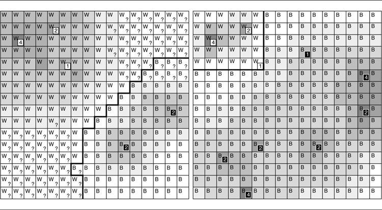
Figure 6.12: Influence map problems with lack of knowledge
When human beings see only partial information, they make force estimations based on a prediction of what units they can’t see. If you see a row of pike men on a medieval battlefield, you may assume there is a row of archers somewhere behind, for example. Unfortunately, it is very difficult to create AI that can accurately predict the forces it can’t see. One approach is to use neural networks with Hebbian learning. A detailed run-through of this example is given in Chapter 7.
Behind influence mapping, the next most common form of tactical analysis deals with the properties of the game terrain. Although it doesn’t necessarily need to work with outdoor environments, the techniques in this section originated for outdoor simulations and games, so the “terrain analysis” name fits. Earlier in the chapter we looked at waypoint tactics in depth. These are more common for indoor environments, although in practice there is almost no difference between the two.
Terrain analysis tries to extract useful data from the structure of the landscape. The most common data to extract are the difficulty of the terrain (used for pathfinding or other movement) and the visibility of each location (used to find good attacking locations and to avoid being seen). In addition, other data, such as the degree of shadow, cover, or the ease of escape, can be obtained in the same way.
Unlike influence mapping, most terrain analyses will always be calculated on a location-by-location basis. For military influence we can use optimizations that spread the influence out starting from the original units, allowing us to use the map flooding techniques later in the chapter. For terrain analysis this doesn’t normally apply.
The algorithm simply visits each location in the map and runs an analysis algorithm for each one. The analysis algorithm depends on the type of information we are trying to extract.
Terrain Difficulty
Perhaps the simplest useful information to extract is the difficulty of the terrain at a location. Many games have different terrain types at different locations in the game. This may include rivers, swampland, grassland, mountains, or forests. Each unit in the game will face a different level of difficulty moving through each terrain type. We can use this difficulty directly; it doesn’t qualify as a terrain analysis because there’s no analysis to do.
In addition to the terrain type, it is often important to take account of the ruggedness of the location. If the location is grassland at a one in four gradient, then it will be considerably more difficult to navigate than a flat pasture.
If the location corresponds to a single height sample in a height field (a very common approach for outdoor levels), the gradient can easily be calculated by comparing the height of a location with the height of neighboring locations. If the location covers a relatively large amount of the level (a room indoors, for example), then its gradient can be estimated by making a series of random height tests within the location. The difference between the highest and the lowest sample provides an approximation to the ruggedness of the location. You could also calculate the variance of the height samples, which may also be faster if well optimized.
Whichever gradient calculation method we use, the algorithm for each location takes constant time (assuming a constant number of height checks per location, if we use that technique). This is relatively fast for a terrain analysis algorithm, and combined with the ability to run terrain analyses offline (as long as the terrain doesn’t change), it makes terrain difficulty an easy technique to use without heavily optimizing the code.
With a base value for the type of terrain and an additional value for the gradient of the location, we can calculate a final terrain difficulty. The combination may use any kind of function—a weighted linear sum, for example, or a product of the base and gradient values. This is equivalent to having two different analyses—the base difficulty and the gradient—and applying a multitiered analysis approach. We’ll look at more issues in combining analyses later in the section on multi-tiered analysis.
There is nothing to stop us from including additional factors into the calculation of terrain difficulty. If the game supports breakdowns of equipment, we might add a factor for how punishing the terrain is. For example, a desert may be easy to move across, but it might take its toll on machinery. The possibilities are bounded only by what kinds of features you want to implement in your game design.
Visibility Map
The second most common terrain analysis I have worked with is a visibility map. There are many kinds of tactics that require some estimation of how exposed a location is. If the AI is controlling a reconnaissance unit, it needs to know locations that can see a long way. If it is trying to move without being seen by the enemy, then it needs to use locations that are well hidden instead.
The visibility map is calculated in the same way as we calculated visibility for waypoint tactics: we check the line of sight between the location and other significant locations in the level.
An exhaustive test will test the visibility between the location and all other locations in the level. This is very time consuming, however, and for very large levels it can take many minutes. There are algorithms intended for rendering large landscapes that can perform some important optimizations, culling large areas of the level that couldn’t possibly be seen. Indoors, the situation is typically better still, with even more comprehensive tools for culling locations that couldn’t possibly be seen. The algorithms are beyond the scope of this book but are covered in most texts on programming rendering engines.
Another approach is to use only a subset of locations. We can use a random selection of locations, as long as we select enough samples to give a good approximation of the correct result.
We could also use a set of “important” locations. This is normally only done when the terrain analysis is being performed online during the game’s execution. Here, the important locations can be key strategic locations (as decided by the influence map, perhaps) or the location of enemy forces.
Finally, we could start at the location we are testing, shoot out rays at a fixed angular interval, and test the distance they travel, as we saw for waypoint visibility checks. This is a good solution for indoor levels, but doesn’t work well outdoors because it is not easy to account for hills and valleys without shooting a very large number of rays.
Regardless of the method chosen, the end point will be an estimate of how visible the map is from the location. This will usually be the number of locations that can be seen, but may be an average ray length if we are shooting out rays at fixed angles.
6.2.4 LEARNING WITH TACTICAL ANALYSES
So far I have described analyses that involve finding information about the game level. The values in the resulting map are calculated by analyzing the game level and its contents.
A slightly different approach has been used successfully to support learning in tactical AI. We start with a blank tactical analysis and perform no calculations to set its values. During the game, whenever an interesting event happens, we change the values of some locations in the map.
For example, suppose we are trying to avoid our character falling into the same trap repeatedly by being ambushed. We would like to know where the player is most likely to lay a trap and where it is best to avoid. While we can perform analysis for cover locations, or ambush waypoints, the human player is often more ingenious than our algorithms and can find creative ways to lay an ambush.
To solve the problem we create a “frag-map.” This initially consists of an analysis where each location gets a zero. Each time the AI sees a character get hit (including itself), it subtracts a number from the location in the map corresponding to the victim. The number to subtract could be proportional to the amount of hit points lost. In most implementations, developers simply use a fixed value each time a character is killed (after all the player doesn’t normally know the amount of hit points lost when another player is hit, so it would be cheating to give the AI that information). We could alternatively use a smaller value for non-fatal hits.
Similarly, if the AI sees a character hit another character, it increases the value of the location corresponding to the attacker. The increase can again be proportional to the damage, or it may be a single value for a kill or non-fatal hit.
Over time we will build up a picture of the locations in the game where it is dangerous to hang about (those with negative values) and where it is useful to stand to pick off enemies (those with positive values). The frag-map is independent of any analysis. It is a set of data learned from experience.
For a very detailed map, it can take a lot of time to build up an accurate picture of the best and worst places. We only find a reasonable value for a location if we have several experiences of combat at that location. We can use filtering (see later in this section) to take the values we do know and expand them out to form estimates for locations we have no experience of.
Frag-maps are suitable for offline learning. They can be compiled during testing to build up a good approximation of the potential for a level. In the final game they will be fixed.
Alternatively, they can be learned online during the game execution. In this case it is usually common to take a pre-learned version as the basis to avoid having to learn really obvious things from scratch. It is also common, in this case, to gradually move all the values in the map toward zero. This effectively “unlearns” the tactical information in the frag-map over time. This is done to make sure that the character adapts to the player’s playing style.
Initially, the character will have a good idea where the hot and dangerous locations are from the pre-compiled version of the map. The player is likely to react to this knowledge, trying to set up attacks that expose the vulnerabilities of the hot locations. If the starting values for these hot locations are too high, then it will take a huge number of failures before the AI realizes that the location isn’t worth using. This can look stupid to the player: the AI repeatedly using a tactic that obviously fails.
If we gradually reduce all the values back toward zero, then after a while all the character’s knowledge will be based on information learned from the player, and so the character will be tougher to beat.
Figure 6.13 shows this in action. In the first diagram we see a small section of a level with the danger values created from play testing. Note the best location to ambush from, A, is exposed from two directions (locations B and C). We have assumed that the AI character gets killed ten times in location A by five attacks from B and C. The second map shows the values that would result if there was no unlearning: A is still the best location to occupy. A frag provides +1 point to the attacker’s location and −1 point to that of the victim; it will take another 10 frags before the character learns its lesson. The third map shows the values that would result if all the values are multiplied by 0.9 before each new frag is logged. In this case location A will no longer be used by the AI; it has learned from its mistakes. In a real game it may be beneficial to forget even more quickly: the player may find it frustrating that it takes even five frags for the AI to learn that a location is vulnerable.

Figure 6.13: Learning a frag-map
If we are learning online, and gradually unlearning at the same time, then it becomes crucial to try to generalize from what the character does know into areas that it has no experience of. The filtering technique later in the section gives more information on how to do this.
6.2.5 A STRUCTURE FOR TACTICAL ANALYSES
So far we’ve looked at the two most common kinds of tactical analyses: influence mapping (determining military influence at each location) and terrain analysis (determining the effect of terrain features at each location).

Figure 6.14: Tactical analyses of differing complexity
Tactical analysis isn’t limited to these concerns, however. Just as we saw for tactical way-points, there may be any number of different pieces of tactical information that we might want to base our decisions on. We may be interested in building a map of regions with lots of natural resources to focus an RTS side’s harvesting/mining activities. We may be interested in the same kind of concerns we saw for waypoints: tracking the areas of shadow in the game to help a character move in stealth. The possibilities are endless.
We can distinguish different types of tactical analyses based on the when and how they need to be updated. Figure 6.14 illustrates the differences.
In the first category are those analyses that calculate unchanging properties of the level. These analyses can be performed offline before the game begins. The gradients in an outdoor landscape will not change, unless the landscape can be altered (some RTS games do allow the landscape to be altered). If the lighting in a level is constant (i.e., you can’t shoot out the lights or switch them off), then shadow areas can often be calculated offline. If your game supports dynamic shadows from movable objects, then this will not be possible.
In the second category are those analyses that change slowly during the course of the game. These analyses can be performed using updates that work very slowly, perhaps only reconsidering a handful of locations at each frame. Military influence in an RTS can often be handled in this way. The coverage of fire and police in a city simulation game could also change quite slowly.
In the third category are properties of the game that change very quickly. To keep up, almost the whole level will need to be updated every frame. These analyses are typically not suited for the algorithms in this chapter. We’ll need to handle rapidly changing tactical information slightly differently.
Updating almost any tactical analysis for the whole level at each frame is too time consuming. For even modestly sized levels it can be noticeable. For RTS games with their larger level sizes, it will often be impossible to recalculate all the levels within one frame’s processing time. No optimization can get around this; it is a fundamental limitation of the approach.
To make some progress, however, we can limit the recalculation to those areas that we are planning to use. Rather than recalculate the whole level, we simply recalculate those areas that are most important. This is an ad hoc solution: we defer working any data out until we know they are needed. Deciding which locations are important depends on how the tactical analysis system is being used.
The simplest way to determine importance is the neighborhood of the AI-controlled characters. If the AI is seeking a defensive location away from the enemy’s line of sight (which is changing rapidly as the enemy move in and out of cover), then we only need to recalculate those areas that are potential movement sites for the characters. If the tactical quality of potential locations is changing fast enough, then we need to limit the search to only nearby locations (otherwise, the target location may end up being in line of sight by the time we get there). This limits the area we need to recalculate to just a handful of neighboring locations.
Another approach to determine the most important locations is to use a second-level tactical analysis, one that can be updated gradually and that will give an approximation to the third-level analysis. The areas of interest from the approximation can then be examined in more depth to make a final decision.
For example, in an RTS, we may be looking for a good location to keep a super-unit concealed. Enemy reconnaissance flights can expose a secret very easily. A general analysis can keep track of good hiding locations. This could be a second-level analysis that takes into account the current position of enemy armor and radar towers (things that don’t move often) or a first-level analysis that simply uses the topography of the level to calculate low-visibility spots. At any time, the game can examine the candidate locations from the lower level analysis and run a more complete hiding analysis that takes into account the current motion of recon flights.
Multi-Layer Analyses
For each tactical analysis the end result is a set of data on a per-location basis: the influence map provides an influence level, side, and optionally a security level (one or two floating point numbers and an integer representing the side); the shadow analysis provides shadow intensity at each location (a single floating point number); and the gradient analysis provides a value that indicates the difficulty of moving through a location (again, a single floating point number).
In Section 6.1 we looked at combining simple tactics into more complex tactical information. The same process can be done for tactical analyses. This is sometimes called multi-layer analysis, and I’ve shown it on the schematic for tactical analyses (Figure 6.14) as spanning all three categories: any kind of input tactical analysis can be used to create the compound information.
Imagine we have an RTS game where the placement of radar towers is critical to success. Individual units can’t see very far alone. To get a good situational awareness we need to build long-distance radar. We need a good method for working out the best locations for placing the radar towers.
Let’s say, for example, that the best radar tower locations are those with the following properties:
• Wide range of visibility (to get the maximum information)
• In a well-secured location (towers are typically easy to destroy)
• Far from other radar towers (no point duplicating effort)
In practice, there may be other concerns also, but we’ll stick with these for now. Each of these three properties is the subject of its own tactical analysis. The visibility tactic is a kind of terrain analysis, and the security is based on a regular influence map.
The distance from other towers is also a kind of influence map. We create a map where the value of a location is given by the distance to other towers. This could be just the distance to the nearest tower, or it might be some kind of weighted value from several towers. We can simply use the influence map function covered earlier to combine the influence of several radar positions.
The three base tactical analyses are finally combined into a single value that demonstrates how good a location is for a radar base.
The combination might be of the form:
where “Security” is a value for how secure a location is. If the location is controlled by another side, this should be zero. “Visibility” is a measure of how much of the map can be seen from the location, and “Distance” is the distance from the nearest tower. If we use the influence formula to calculate the influence of nearby towers, rather than the distance to them, then the formula may be of the form:
although we need to make sure the influence value is never zero.
Figure 6.15 shows the three separate analyses and the way they have been combined into a single value for the location of a radar tower. Even though the level is quite small, we can see that there is a clear winner for the location of the next radar tower.
There is nothing special in the way the three terms have been combined here, and there may be better ways to put them together, using a weighted sum, for example (although then care needs to be taken not to try to build on another side’s territory). The formula for combining the layers needs to be created by the developer, and in a real game, it will involve fine tuning and tweaking.
I have found throughout my career building game AI that whenever something needs tweaking, it is almost essential to be able to visualize it in the game. In this case I would support a mode where the tower-placement value can be displayed in the game at any time (this would only be part of the debug version, not the final distribution) so the results of combining each feature can be clearly seen.

Figure 6.15: The combined analyses
When to Combine Things
Combining tactical analyses is exactly the same as using compound tactics with waypoints: we can choose when to perform the combination step.
If the base analyses are all calculated offline, then we have the option of performing the combination offline also and simply storing its results. This might be the best option for a tactical analysis of terrain difficulty: combining gradient, terrain type, and exposure to enemy fire, for example.
If any of the base analyses are changed during the game, then the combined value needs to be recalculated. In our example above, both the security level and distance to other towers change over the course of the game, so the whole analysis needs to be recalculated during the game also.
Considering the hierarchy of tactical analyses introduced earlier, the combined analysis will be in the same category as the highest base analysis it relies on. If all the base analyses are in category one, then the combined value will also be in category one. If we have one base analysis in category one and two base analyses in category two (as in our radar example), then the overall analysis will also be in category two. We’ll need to update it during the game, but not very rapidly.
For analyses that aren’t used very often, we could also calculate values only when needed. If the base analyses are readily available, we can query a value and have it created on the fly. This works well when the AI is using the analysis a location at a time—for example, for tactical pathfinding. If the AI needs to consider all the locations at the same time (to find the highest scoring location in the whole graph), then it may take too long to perform all the calculations on the fly. In this case it is better to have the calculations being performed in the background (possibly taking hundreds of frames to completely update) so that a complete set of values is available when needed.
Building a Tactical Analysis Server
If your game relies heavily on tactical analyses, then it is worth investing the implementation time in building a tactical analysis server that can cope with each different category of analysis. Personally, I have only needed to do this once, but building a common application programming interface (API) that allowed any kind of analysis (as a plug-in module), along with any kind of combination, allowed a very generic visualization system to be built, and really helped speed up the addition and debugging of new tactical concerns. Unlike the example I gave earlier, in this system only weighted linear combinations of analyses were supported. This made it easier to build a simple data file format that showed how to combine primitive analyses into compound values.
The server should support distributing updates over many frames, calculating some values offline (or during loading of the level) and calculating values only when they are needed. This can easily be based on the time-slicing and resource management systems discussed in Chapter 10, Execution Management (this was our approach, and it worked well).
The techniques developed in Chapter 4 are used to split the game level into regions. In particular, tiles or Dirichlet domains are widely used, with points of visibility and navigation meshes being less practical. Individual tiles in a tile-based game may be too small for tactical analysis, and tiles may benefit from being grouped together into larger regions.
The same techniques used for pathfinding can be used to calculate Dirichlet domains in influence maps. When we have a tile-based level, however, these two different sets of regions can be difficult to reconcile. Fortunately, there is a technique for calculating the Dirichlet domains on tile-based levels. This is map flooding, and it can be used to work out which tile locations are closer to a given location than any other. Beyond Dirichlet domains, map flooding can be used to move properties around the map, so the properties of intermediate locations can be calculated.
Starting from a set of locations with some known property (such as the set of locations where there is a unit), we’d like to calculate the properties of every other location. As a concrete example we’ll consider an influence map for a strategy game: a location in the game belongs to the player who has the nearest city to that location. This would be an easy task for a map flooding algorithm. To show off a little more of what the algorithm can do, we can make things harder by adding some complications:
• Each city has a strength, and stronger cities tend to have larger areas of influence than weaker ones.
• The region of a city’s influence should extend out from the city in a continuous area. It can’t be split into multiple regions.
• Cities have a maximum radius of influence that depends on the city’s strength.
We’d like to calculate the territories for the map. For each location we need to know the city that it belongs to (if any).
The Algorithm
We will use a variation of the Dijkstra algorithm we saw in Chapter 4.
The algorithm starts with the set of city locations. We’ll call this the open list. Internally, we keep track of the controlling city and strength of influence for each location in the level.
At each iteration the algorithm takes the location with the greatest strength and processes it. We’ll call this the current location. Processing the current location involves looking at the location’s neighbors and calculating the strength of influence for each location for just the city recorded in the current node.
This strength is calculated using an arbitrary algorithm (i.e., we will not care how it is calculated). In most cases it will be the kind of drop-off equation we saw earlier in the chapter, but it could also be generated by taking the distance between the current and neighboring locations into account. If the neighboring location is beyond the radius of influence of the city (normally implemented by checking if the strength is below some minimum threshold), then it is ignored and not processed further.
If a neighboring location already has a different city registered for it, then the currently recorded strength is compared with the strength of influence from the current location’s city. The highest strength wins, and the city and strength are set accordingly. If it has no existing city recorded, then the current location’s city is recorded, along with its influence strength.
Once the current location is processed, it is placed on a new list called the closed list. When a neighboring node has its city and strength set, it is placed on the open list. If it was already on the closed list, it is first removed from there. Unlike for the pathfinding version of the algorithm, we cannot guarantee that an updating location will not be on the closed list, so we have to make allowances for removing it. This is because we are using an arbitrary algorithm for the strength of influence.
Pseudo-Code
Other than changes in nomenclature, the algorithm is very similar to the pathfinding Dijkstra algorithm.


Data Structures and Interfaces
This version of Dijkstra takes as input a map that is capable of generating the neighboring locations of any location given. It should be of the following form:

In the most common case where the map is grid based, this is a trivial algorithm to implement and can even be included directly in the Dijkstra implementation for speed.
The algorithm needs to be able to find the position and strength of influence of each of the cities passed in. For simplicity, I’ve assumed each city is an instance of some city class that is capable of providing this information directly. The class has the following format:
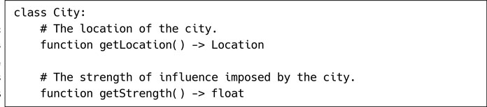
Finally, both the open and closed lists behave just like they did when we used them for pathfinding. Refer to Chapter 4, Section 4.2, for a complete rundown of their structure. The only difference is that I’ve replaced the smallestElement method with a largestElement method. In the pathfinding case we were interested in the location with the smallest path-so-far (i.e., the location closest to the start). This time we are interested in the location with the largest strength of influence (which is also a location closest to one of the start positions: the cities).
Performance
Just like the pathfinding Dijkstra, this algorithm on its own is O(nm) in time, where n is the number of locations that belong to any city, and m is the number of neighbors for each location. Unlike before, the worst case memory requirement is O(n) only, because we ignore any location not within the radius of influence of any city.
Also like in the pathfinding version, however, the data structures use algorithms that are nontrivial. See Chapter 4, Section 4.3 for more information on the performance and optimization of the list data structures.
Image blur algorithms are a very popular way to update analyses that involve spreading values out from their source. Influence maps in particular have this characteristic, but so do other proximity measures. Terrain analyses can sometimes benefit, but they typically don’t need the spreading-out behavior.
Similar algorithms are used outside of games also. They are used in physics to simulate the behavior of many different kinds of fields and form the basis of models of heat transfer around physical components.
The blur effect inside your favorite image editing package is one of a family of convolution filters. Convolution is a mathematical operation that we will not need to consider in this book. For more information on the mathematics behind filters, I’d recommend Digital Image Processing [17]. Convolution filters go by a variety of other names, too, depending on the field you are most familiar with: kernel filters, impulse response filters, finite element simulation,1 and various others.
The Algorithm
All convolution filters have the same basic structure: we define an update matrix to tell us how the value of one location in the map gets updated based on its own value and that of its neighbors. For a square tile-based level, we might have a matrix that looks like the following:
This is interpreted by taking the central element in the matrix (which, therefore, must have an odd number of rows and columns) as referring to the tile we are interested in. Starting with the current value of that location and its surrounding tiles, we can work out the new value by multiplying each value in the map by the corresponding value in the matrix and summing the results. The size of the filter is the number of neighbors in each direction. In the example above we have a filter size of one.
So if we have a section of the map that looks like the following:
and we are trying to work out a new value for the tile that currently has the value 4 (let’s call it ν). The following calculation is performed:
We repeat this process for each location in the map, applying the matrix and calculating a new value. We need to be careful, however. If we just start at the top left corner of the map and work our way through in reading order (i.e., left to right, then top to bottom), we will be consistently using the new value for the map locations to the left, above, and diagonally above and left, but the old values for the remaining locations. This asymmetry can be acceptable, but very rarely. It is better to treat all values the same.
To do this we have two copies of the map. The first is our source copy. It contains the old values, and we only read from it. As we calculate each new value, it is written to the new destination copy of the map. At the end of the process the destination copy contains an accurate update of the values. In our example, the values will be:
rounded to three decimal places.
To make sure the influence propagates from a location to all the other locations in the map, we need to repeat this process many times. Before each repeat, we set the influence value of each location where there is a unit.
If there are n tiles in each direction on the map (assuming a square tile-based map), then we need up to n passes through the filter to make sure all values are correct. If the source values are in the middle of the map, we may only need half this number.
If the sum total of all the elements in our matrix is one, then the values in the map will eventually settle down and not change over additional iterations. As soon as the values settle down, we need no more iterations.
In a game, where time is of the essence, we don’t want to spend a long time repeatedly applying the filter to get a correct result. We can limit the number of iterations through the filter. Often, you can get away with applying one pass through the filter each frame and using the values from previous frames. In this way the blurring is spread over multiple frames. If you have fast-moving characters on the map, however, you may still be blurring their old location long after they have moved, which may cause problems. It is worth experimenting to get the best balance of performance and quality.
Boundaries
Before we implement the algorithm, we need to consider what happens at the edges of the map. Here we are no longer able to apply the matrix because some of the neighbors for the edge tile do not exist.
There are two approaches to this problem: modify the matrix or modify the map.
We could modify the matrix at the edges so that it only includes the neighbors that exist. At the top left-hand corner, for example, our blur matrix becomes:
and
on the bottom edge.
This approach is the most correct and will give good results. Unfortunately, it involves working with nine different matrices and switching between them at the correct time. The regular convolution algorithm given below can be very comprehensively optimized to take advantage of single instruction, multiple data (SIMD), processing several locations at the same time, especially on GPU hardware. If we need to keep switching matrices, these optimizations are no longer easy to achieve, and we lose a good deal of the speed (in my experiments for this book, the matrix-switching version can take 1.5 to 5 times as long).
The second alternative is to modify the map. We do this by adding a border around the game locations and clamping their values (i.e., they are never processed during the convolution algorithm; therefore, they will never change their value). The locations in the map can then use the regular algorithm and draw data from tiles that only exist in this border.
This is a fast and practical solution, but it can produce edge artifacts. Because we have no way of knowing what the border values should be set at, we choose some arbitrary value (say zero). The locations that neighbor the border will consistently have a contribution of this arbitrary value added to them. If the border is all set to zero, for example, and a high-influence character is next to it, its influence will be pulled down because the edge locations will be receiving zero-valued contributions from the invisible border.
This is a common artifact to see. If you visualize the influence map as color density, it appears to have a paler color halo around the edge. The same thing will occur regardless of the value chosen for the border. It can be alleviated by increasing the size of the border and allowing some of the border values to be updated normally (even though they aren’t part of the game level). This doesn’t solve the problem, but can make it less visible.
Pseudo-Code
The convolution algorithm can be implemented in the following way:
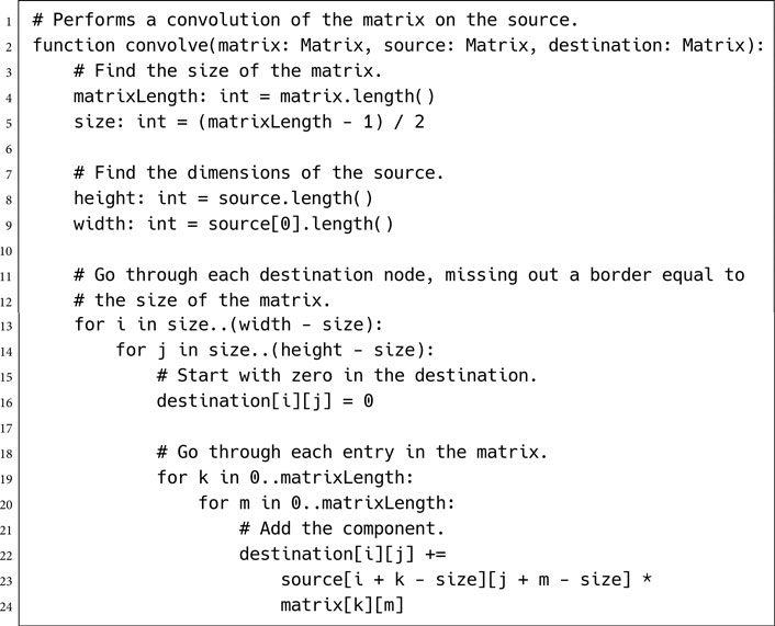
To apply multiple iterations of this algorithm, we can use a driver function that looks like the following:

although, as we’ve already seen, this is not commonly used.
Data Structures and Interfaces
This code uses no peculiar data structures or interfaces. It requires both the matrix and the source data as a rectangular array of arrays (containing numbers, of whatever type you need).
The matrix parameter needs to be a square matrix, but the source matrix can be of whatever size. A destination matrix of the same size as the source matrix is also passed in, and its contents are altered.
Implementation Notes
The algorithm is a prime candidate for optimizing using SIMD hardware, especially passing to the GPU. The same calculation is being performed on different data, and this can be parallelized. Even if you choose to run it on the CPU, a good optimizing compiler that can take advantage of SIMD processing is likely to automatically optimize these inner loops for you.
Performance
The algorithm is O(whs2) in time, where w is the width of the source data, h is its height, and s is the size of the convolution matrix. It is O(wh) in memory, because it requires a copy of the source data in which to write updated values.
If memory is a problem, it is possible to split this down and use a smaller temporary storage array, calculating the convolution one chunk of the source data at a time. This approach involves revisiting certain calculations, thus decreasing execution speed.
Filters
So far we’ve only seen one possible filter matrix. In image processing there is a whole wealth of different effects that can be achieved through different filters. Most of them are not useful in tactical analyses.
We’ll look at two in this section that have practical use: the Gaussian blur and the sharpening filter. Gonzalez and Woods [17] contains many more examples, along with comprehensive mathematical explanations of how and why certain matrices create certain effects.
Gaussian Blur
The blur filter we looked at earlier is one of a family called Gaussian filters. They blur values, spreading them around the level. As such they are ideal for spreading out influence in an influence map.
For any size of filter, there is one Gaussian blur filter. The values for the matrix can be found by taking two vectors made up of elements of the binomial series; for the first few values these are
We then calculate their outer product. So for the Gaussian filter of size two, we get:
We could use this as our matrix, but the values in the map would increase dramatically each time through. To keep them at the same average level, and to ensure that the values settle down, we divide through by the sum of all the elements. In our case this is 256:
If we run this filter over and over on an unchanging set of unit influences, we will end up with the whole level at the same influence value (which will be low). The blur acts to smooth out differences, until eventually there will be no difference left.
We could add in the influence of each unit each time through the algorithm. This would have a similar problem: the influence values would increase at each iteration until the whole level had the same influence value as the units being added.
To solve these problems we normally introduce a bias: the equivalent of the unlearning parameter we used for frag-maps earlier. At each iteration we add the influence of the units we know about and then remove a small amount of influence from all locations. The total removed influence should be the same as the total influence added. This ensures that there is no net gain or loss over the whole level, but that the influence spreads correctly and settles down to a steady state value.
Figure 6.16 shows the effect of our size-two Gaussian blur filter on an influence map. The algorithm ran repeatedly (adding the unit influences each time and removing a small amount) until the values settled down.
Separable Filters
The Gaussian filter has an important property that we can use to speed up the algorithm. When we created the filter matrix, we did so using the outer product of two identical vectors:
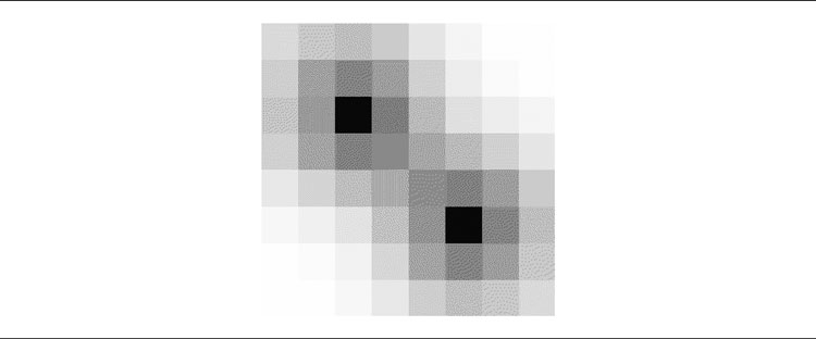
Figure 6.16: Screenshot of a Gaussian blur on an influence map
This means that, during an update, the values for locations in the map are being calculated by the combined action of a set of vertical calculations and horizontal calculations. What is more, the vertical and horizontal calculations are the same. We can separate them out into two steps: first an update based on neighboring vertical values and second using neighboring horizontal values.
For example, let’s return to our original example. We have part of the map that looks like the following:
and, what we now know is a Gaussian blur, with the matrix:
We replace the original updated algorithm with a two-step process. First, we work through each column and apply just the vertical vector, using the components to multiply and sum the values in the table just as before. So if the 1 value in our example is called w, then the new value for w is given by:
We repeat this process for the whole map, just as if we had a whole filter matrix. After this update we end up with:
After this is complete, we then go through again performing the horizontal equivalent (i.e., using the matrix [1 2 1]). We end up with:
exactly as before.
The pseudo-code for this algorithm looks like the following:

We are passing in two vectors, the two vectors whose outer product gives the convolution matrix. In the examples above this has been the same vector for each direction, although it could just as well be different. We are also passing in another array of arrays, called temp, again the same size as the source data. This will be used as temporary storage in the middle of the update.
Rather than doing nine calculations (a multiplication and addition in each) for each location in the map, we’ve done only six: three vertical and three horizontal. For larger matrices the saving is even larger, a size 3 matrix would take 25 calculations the long way or 10 if it were separable. It is therefore O(whs) in time, rather than the O(whs2) of the previous version. It doubles the amount of temporary storage space needed, however, although it is still O(wh).
In fact, if we are restricted to Gaussian blurs, there is a faster algorithm (called SKIPSM, discussed in Waltz and Miller [75]) that can be implemented in assembly and run very quickly on the CPU. It is not designed to take full advantage of SIMD hardware, however. So in practice a well-optimized version of the algorithm above will perform almost as well and will be considerably more flexible.
It is not only Gaussian blurs that are separable, although most convolution matrices are not. If you are writing a tactical analysis server that can be used as widely as possible, then you should support both algorithms. The remaining filters in this chapter are not separable, so they require the long version of the algorithm.
The Sharpening Filter
Rather than blur influence out, we might want to concentrate it in. If we need to understand where the central hub of our influence is (to determine where to build a base, for example), we could use a sharpening filter. Sharpening filters act in the opposite way of blur filters: concentrating the values in the regions that already have the most.
A matrix for the sharpening filter has a central positive value surrounded by negative values; for example,
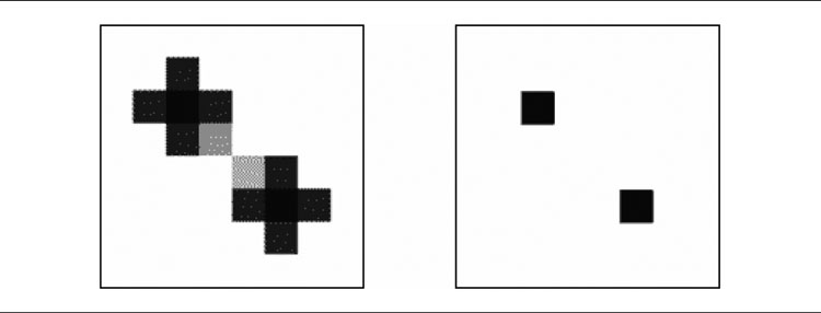
Figure 6.17: Screenshot of a sharpening filter on an influence map
and more generally, any matrix of the form:
where a, b, and c are any positive real numbers and typically c < b.
In the same way as for the Gaussian blur, we can extend the same principle to larger matrices. In each case, the central value will be positive, and those surrounding it will be negative.
Figure 6.17 shows the effect of the first sharpening matrix shown above. In the first part of the figure, an influence map has been sharpened once only.
Because the sharpening filter acts to reduce the distribution of influence, if we run it multiple times we are likely to end up with an uninspiring result. In the second part of the figure the algorithm has been run for more iterations (adding the unit influences each time and removing a bias quantity) until the values settle down. You can see that the only remaining locations with any influence are those with units in them (i.e., those we already know the influence of).
Where sharpening filters can be useful for terrain analysis, they are usually applied only a handful of times and are rarely run to a steady state.
Cellular automata are update rules that generate the value at one location in the map based on the values of other surrounding locations. This is an iterative process: at each iteration, values are calculated based on the surrounding values at the previous iteration. This makes it a dynamic process that is more flexible than map flooding and can give rise to useful emergent effects.

Figure 6.18: A cellular automaton
In academia, cellular automata gained attention as a biologically plausible model of computing (although many commentators have subsequently shown why they aren’t that biologically plausible), but with little practical use.
They have been used in only a handful of games, to my knowledge, mostly city simulation games, with the canonical example being SimCity [135], as described by its creator Will Wright in several conference talks. In SimCity they aren’t used specifically for the AI; they are used to model changing patterns in the way the city evolves. I have used a cellular automaton to identify tactical locations for snipers in a small simulation, and I suspect they can be used more widely in tactical analysis.
Figure 6.18 shows one cell in a cellular automaton. It has a neighborhood of locations whose values it depends on. The update can be anything from a simple mathematical function to a complex set of rules. The figure shows an intermediate example.
Note, in particular, that if we are dealing with numeric values at each location, and the update rules are a single mathematical function, then we have a convolution filter, just as we saw in the previous section. In fact, convolution filters are just one example of a cellular automaton. This is not widely recognized, and most people tend to think of cellular automata solely in terms of discrete values at each location and more complex update rules.
Typically, the values in each surrounding location are first split into discrete categories. They may be enumerated values to start with (the type of building in a city simulation game, for example, or the type of terrain for an outdoor RTS). Alternatively, we may have to split a real number into several categories (splitting a gradient into categories for “flat,” “gentle,” “steep,” and “precipitous,” for example).
Given a map where each location is labeled with one category from our set, we can apply an update rule on each location to give the category for the next iteration. The update for one location depends only on the value of locations at the previous iteration. This means the algorithm can update locations in any order.
Cellular Automata Rules
The most well-known variety of cellular automata has an update rule that gives an output, based on the numbers of its neighbors in each category. In academic CAs, the categories are often ‘off ’ and ‘on’, and the rule switches a location (often known as a “cell”) on or off depending on the number of on neighbors it has. Figure 6.18 shows such a rule, for two categories, but in this case with more game significance. In the rule, it states that a location that borders at least four secure locations should be treated as secure.
Running the same rule over all the locations in a map allows us to turn an irregular zone of security (where the AI may mistakenly send units into the folds, only to have the enemy easily flank them) into a more convex pattern.
Cellular automaton rules could be created to take account of any information available to the AI. They are designed to be very local, however. A simple rule decides the characteristic of a location based only on its immediate neighbors. The complexity and dynamics of the whole automaton arise from the way these local rules interact. If two neighboring locations change their category based on each other, then the changes can oscillate backward and forward. In many cellular automata, even more complex behaviors can arise, including never-ending sequences that involve changes to the whole map.
Most cellular automata are not directional; they don’t treat one neighbor any differently from any other. If a location in a city game has three neighboring high-crime areas, we might have a rule that says the location is also a high-crime zone. In this case, it doesn’t matter which of the location’s neighbors are high crime as long as the numbers add up. This enables the rule to be used in any location on the map.
Edges can pose a problem, however. In academic cellular automata, the map is considered to be either infinite or toroidal (i.e., the top and the bottom are joined, as are the left and right edges). Either approach gives a map where every location has the same number of neighbors. In a real game this will not be the case. In fact, many times we will not be working on a grid-based map at all, and so the number of neighbors might change from location to location.
To avoid having different behavior at different locations, we can use rules that are based on larger neighborhoods (not just locations that touch the location in question) and proportions rather than absolute numbers. We might have a rule that says if at least 25% of neighboring locations are high-crime areas then a location is also high crime, for example.
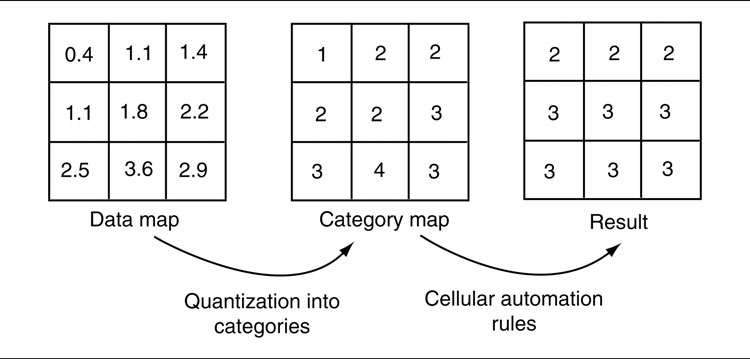
Figure 6.19: Updating a cellular automaton
Running a Cellular Automaton
We need two copies of the tactical analysis to allow the cellular automaton to update. One copy stores the values at the previous iteration, and the other copy stores the updated values. We can alternate which copy is which and repeatedly use the same memory.
Each location is considered in sequence (in any order, as we’ve seen), taking its input from its neighboring location and placing its output in the new copy of the analysis.
If we need to split a real-valued analysis into categories, this is often done as a preprocessing step first. A third copy of the map is kept, containing integers that represent the enumerated categories. The correct category is filled in each location from the real-numbered source data. Finally, the cellular automaton update rule runs as normal, converting its category output into a real number for writing into the destination map. This process is shown in Figure 6.19.
If the update is a simple mathematical function of its inputs, without branches, then it can often be written as parallel code that can be run on either the graphics card or a specialized vector mathematics unit. This can speed up the execution dramatically, as long as there is some headroom on those chips (if the graphics processing is taking every ounce of their power, then you may as well run the simulation on the CPU, of course).
In most cases, however, update functions of cellular automata tend to be heavily branched; they consist of lots of switch or if statements. This kind of processing isn’t as easily parallelized, and so it is often performed in series on the main CPU, with a corresponding performance decrease. Some cellular automata rule sets (in particular, Conway’s “The Game of Life”: the most famous set of rules, but practically useless in a game application) can be easily rewritten without branches and have been implemented in a highly efficient parallel manner. Unfortunately, it is not always sensible to do so because the rewrites can take longer to run than a good branched implementation.
The Complexity of Cellular Automata
The behavior of a cellular automaton can be extremely complex. In fact, for some rules the behavior is so complex that the patterns of values become a programmable computer. This is part of the attraction of using the method: we can create sets of rules that produce almost any kind of pattern we like.
Unfortunately, because the behavior is so complex, there is no way we can accurately predict what we are going to see for any given rule set. For some simple rules it may be obvious. However, even very simple rules can lead to extraordinarily complex behaviors. The rule for the famous “The Game of Life” is very simple, yet produces completely unpredictable patterns. 2
In game applications we don’t need this kind of sophistication. For tactical analyses we are only interested in generating properties of one location from that of neighboring locations. We would like the resulting analysis to be stable. After a while, if the base data (like the positions of units or the layout of the level) stay the same, then the values in the map should settle down to a consistent pattern.
Although there are no guaranteed methods for creating rules that settle in this way, I have found that a simple rule of thumb is to set only one threshold in rules. In Conway’s “The Game of Life,” for example, a location can be on or off. It comes on if it has three on neighbors, and it goes off if it has fewer than two or more than four (there are eight neighbors for each cell in the grid). It is this “band” of two to three neighbors that causes the complex and unpredictable behavior. If the rules simply made locations switch on when they had three or more neighbors, then the whole map would rapidly fill up (for most starting configurations) and would be quite stable.
Bear in mind that you don’t need to introduce dynamism into the game through complex rules. The game situation will be changing as the player affects it. Often, you just want fairly simple rules for the cellular automaton: rules that would lead to boring behavior if the automaton was the only thing running in the game.
Applications and Rules
Cellular automata are a broad topic, and their flexibility induces option paralysis. It is worth looking through a few of their applications and the rules that support them.
Area of Security
Earlier in the chapter I described a set of cellular automata rules that expand an area of security to give a smoother profile, less prone to obvious mistakes in unit placement. It is not suitable for use on the defending side’s area of control, but is useful for the attacking side because it avoids falling foul of a number of simple counterattack tactics.
The rule is simple:
A location is secure if at least four of its eight neighbors (or 50% for edges) are secure.
Building a City
SimCity uses a cellular automaton to work out the way buildings change depending on their neighborhood. A residential building in the middle of a run-down area will not prosper and may fall derelict, for example. SimCity’s urban model is complex and highly proprietary. While I can guess some of the rules, I have no idea of their exact implementation.
A less well-known game, Otostaz [178], uses exactly the same principle, but its rules are simpler. In the game, a building appears on an empty patch of land when it has one square containing water and one square containing trees. This is a level-one building. Taller buildings come into being on squares that border two buildings of the next smaller size, or three buildings of one size smaller, or four buildings of one size smaller still.
So a level-two building appears on a patch of land when it has two neighboring level-one buildings. A level-three building needs two level-two buildings or three level-one buildings, and so on. An existing building doesn’t ever degrade on its own (although the player can remove it), even if the buildings that caused it to generate are removed. This provides the stability to avoid unstable patterns on the map.
This is a gameplay, rather than an AI, use of the cellular automata, but the same thing can be implemented to build a base in an RTS. Typically, an RTS has a flow of resources: raw materials need to be collected, and there needs to be a balance of defensive locations, manufacturing plants, and research facilities.
We could use a set of rules such as:
1. A location near raw materials can be used to build a defensive building.
2. A location bordered by two defensive positions may be used to build a basic building of any type (training, research, and manufacturing).
3. A location bounded by two basic buildings may become an advanced building of a different type (so we don’t put all the same types of technology in one place, vulnerable to a single attack).
4. Very valuable facilities should be bordered by two advanced buildings.
Tactical pathfinding combines the tactical analyses we’ve seen earlier in the chapter with the pathfinding techniques from Chapter 4. It can provide quite impressive results when characters in the game move, taking account of their tactical surroundings, staying in cover, and avoiding enemy lines of fire and common ambush points.
Tactical pathfinding has an unfair reputation for being significantly more sophisticated than regular pathfinding. As a marketing feature that may be a benefit, but if it dissuades programmers from attempting implementation, the reputation is unfortunate. In reality it is no different at all from regular pathfinding. The same pathfinding algorithms are used on the same kind of graph representation. The only modification is that the cost function is extended to include tactical information as well as distance or time.
The cost for moving along a connection in the graph should be based on both distance/time (otherwise, we might embark on exceptionally long routes) and how tactically sensible the maneuver is.
The cost of a connection is given by a formula of the following type:
where D is the distance of the connection (or time or other non-tactical cost function—I will refer to this as the base cost of the connection); wi is a weighting factor for each tactic supported in the game; Ti is the tactical quality for the connection, again for each tactic; and i is the number of tactics being supported. We’ll return to the choice of the weighting factors below.
The only complication in this is the way tactical information is stored in a game. As we have seen so far in this chapter, tactical information is normally stored on a per-location basis. We might use tactical waypoints or a tactical analysis, but in either case the tactical quality is held for each location.
To convert location-based information into connection-based costs, we normally average the tactical quality of each of the locations that the connection connects. This works on the assumption that the character will spend half of its time in each region and so should benefit or suffer half of the tactical properties of each.
This assumption is good enough for most games, although it can produce poor results for some level data. Figure 6.20 shows a connection between two locations with good cover. The connection, however, is very exposed, and the longer route around is likely to be much better in practice.

Figure 6.20: Averaging the connection cost sometimes causes problems
6.3.2 TACTIC WEIGHTS AND CONCERN BLENDING
In the equation for the cost of a connection, the real-valued quality for each tactic is multiplied by a weighting factor before being summed into the final cost value. The choice of weighting factors controls the kinds of routes taken by the character.
We could also use a weighting factor for the base cost, but this would be equivalent to changing the weighting factors for each of the tactics. A 0.5 weight for the base cost can be achieved by multiplying each of the tactic weights by 2, for example. I will not use a separate weight for the base cost in this chapter, but you may find it more convenient to have one in your implementation.
If a tactic has a high weight, then locations with that tactical property will be avoided by the character. This might be the case for ambush locations or difficult terrain, for example. Conversely, if the weight is a large negative value, then the character will favor locations with a high value for that property. This would be sensible for cover locations or areas under friendly control, for example.
Care needs to be taken to make sure that no possible connection in the graph can have a negative overall weight. If a tactic has a large negative weight and a connection has a small base cost with a high value for the tactic, then the resulting overall cost may be negative. As we saw in Chapter 4, negative costs are not supported by normal pathfinding algorithms such as A*. Weights can be chosen so that no negative value can occur, although that is often easier said than done. As a safety net, it is worth specifically limiting the cost value returned so that it is always positive. This adds additional processing time and can also lose lots of tactical information. If the weights are badly chosen, many different connections might be mapped to negative values: simply limiting them so they give a positive result loses any information on which connections are better than the others (they all appear to have the same cost).
Speaking from bitter experience, I would advise you at the very least to include an assert or other debugging message to tell you if a connection arises with a negative cost. A bug resulting from a negative weight can be tough to track down (it may only appear in certain very specific gameplay circumstances that can be hard to replicate, and normally results in the pathfinding never returning a result, but it can cause much more subtle bugs, too).
We can calculate the costs for each connection in advance and store them with the pathfinding graph. There will be one set of connection costs for each set of tactic weights.
This works okay for static features of the game such as terrain and visibility. It cannot take into account the dynamic features of the tactical situation: the balance of military influence, cover from known enemies, and so on. To do this we need to apply the cost function each time the connection cost is requested (we can cache the cost value for multiple queries in the same frame, of course).
Performing the cost calculations when they are needed slows down pathfinding significantly. The cost calculation for a connection is in the lowest loop of the pathfinding algorithm, and any slowdown is usually quite noticeable. There is a trade-off. Is the advantage of better tactical routes for your characters outweighed by the extra time they need to plan the route in the first place?
As well as responding to changing tactical situations, performing the cost calculations for each frame allows great flexibility to model different personalities in different characters.
In a real-time strategy game, for example, we might have reconnaissance units, light infantry, and heavy artillery. A tactical analysis of the game map might provide information on difficulty of terrain, visibility, and the proximity of enemy units.
The reconnaissance units can move fairly efficiently over any kind of terrain, so they weight the difficulty of terrain with a small positive weight. They are keen to avoid enemy units, so they weight the proximity of enemy units with a large positive value. Finally, they need to find locations with large visibility, so they weight this with a large negative value.
The light infantry units have slightly more difficulty with tough terrain, so their weight is a small positive value, higher than that of the reconnaissance units. Their purpose is to engage the enemy. However, they would rather avoid unnecessary engagements, so they use a small positive weight for enemy proximity (if they were actively seeking combat, they’d use a negative value here). They would rather move without being seen, so they use a small positive weight for visibility.
Heavy artillery units have a different set of weights again. They cannot cope with tough terrain, so they use a large positive weight for difficult areas of the map. They also are not good in close encounters, so they have large positive weights for enemy proximity. When exposed, they are a prime target and should move without being seen (they can attack from behind a hill quite successfully), so they also use a large positive weight for visibility.
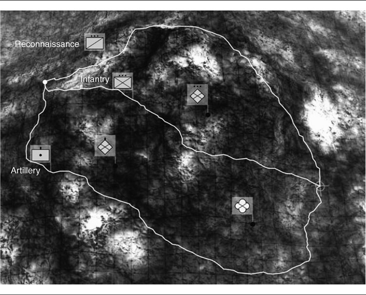
Figure 6.21: Screenshot of the planning system showing tactical pathfinding
These three routes are shown in Figure 6.21, a screenshot for a three-dimensional (3D) level. The black dots in the screenshot show the location of enemy units.
The weights don’t need to be static for each unit type. We could tailor the weights to a unit’s aggression. An infantry unit might not mind enemy contact if it is healthy, but might increase the weight for proximity when it is damaged. That way if the player orders a unit back to base to be healed, the unit will naturally take a more conservative route home.
Using the same source data, the same tactical analyses, and the same pathfinding algorithm, but different weights, we can produce completely different styles of tactical motion that display clear differences in priority between characters.
6.3.3 MODIFYING THE PATHFINDING HEURISTIC
If we are adding and subtracting modifiers to the connection cost, then we are in danger of making the heuristic invalid. Recall that the heuristic is used to estimate the length of the shortest path between two points. It should always return less than the actual shortest path length. Otherwise, the pathfinding algorithm might settle for a sub-optimal path.
We ensured that the heuristic was valid by using a Euclidean distance between two points: any actual path will be at least as long as the Euclidean distance and will usually be longer. With tactical pathfinding we are no longer using the distance as the cost of moving along a connection: subtracting the tactical quality of a connection may bring the cost of the connection below its distance. In this case, a Euclidean heuristic will not work.
In practice, I have only come across this problem once. In most cases, the additions to the cost outweigh the subtractions for the majority of connections (you can certainly engineer the weights so that this is true). The pathfinder will disproportionately tend to avoid the areas where the additions don’t outweigh the subtractions. These areas are associated with very good tactical areas, and it has the effect of downgrading the tendency of a character to use them. Because the areas are likely to be exceptionally good tactically, the fact that the character treats them as only very good (not exceptionally good) is usually not obvious to the player.
The case where I found problems was in a character that weighted most of the tactical concerns with a fairly large negative weight. The character seemed to miss obviously good tactical locations and to settle for mediocre locations. In this case, I used a scaled Euclidean distance for the heuristic, simply multiplying it by 0.5. This produced slightly more fill (see Chapter 4 for more information about fill), but it resolved the issue.
6.3.4 TACTICAL GRAPHS FOR PATHFINDING
Influence maps (or any other kind of tactical analysis) are ideal for guiding tactical pathfinding. The locations in a tactical analysis form a natural representation of the game level, especially in outdoor levels. In indoor levels, or for games without tactical analyses, we can use the waypoint tactics covered at the start of this chapter.
In either case the locations alone are not sufficient for pathfinding. We also need a record of the connections between them. For waypoint tactics that include topological tactics, we may have these already. For regular waypoint tactics and most tactical analyses, we are unlikely to have a set of connections.
We can generate connections by running movement checks or line-of-sight checks between waypoints or map locations. Locations that can be simply moved between are candidates for maneuvers in a planned route. Chapter 4 has more details about the automatic construction of connections between sets of locations.
The most common graph for tactical pathfinding is the grid-based graph used in RTS games. In this case the connections can be generated very simply: a connection exists between two locations if the locations are adjacent. This may be modified by not allowing connections between locations when the gradient is steeper than some threshold or if either location is occupied by an obstacle. More information on grid-based pathfinding graphs can also be found in Chapter 4.

Figure 6.22: Adding waypoints that are not tactically sensible
6.3.5 USING TACTICAL WAYPOINTS
Tactical waypoints, unlike tactical analysis maps, have tactical properties that refer to a very small area of the game level. As we saw in the section on automatically placing tactical way-points, a small movement from a waypoint may produce a dramatic change in the tactical quality of the location.
To make sensible pathfinding graphs it is almost always necessary to add additional way-points at locations that do not have peculiar tactical properties. Figure 6.22 shows a set of tactical locations in part of a level; none of these can be easily reached from any of the others. The figure shows the additional waypoints needed to connect the tactical locations and to form a sensible graph for pathfinding.
The simplest way to achieve this is to superimpose the tactical waypoints onto a regular pathfinding graph. The tactical locations need to be linked into their adjacent pathfinding nodes, but the basic graph provides the ability to move easily between different areas of the level.
The developers I have seen using indoor tactical pathfinding have all included the placement of tactical waypoints into the same level design process used to place nodes for the pathfinding (normally using Dirichlet domains for quantization, or navigation meshes with additional manually specified nodes). By allowing the level designer the ability to mark pathfinding nodes with tactical information, the resulting graph can be used for both simple tactical decision making and for full-blown tactical pathfinding.
So far in this book I have presented techniques in the context of controlling a single character. Increasingly, games feature multiple characters who have to cooperate together to get their job done. This can be anything from a whole side in a real-time strategy game to squads or pairs of individuals in a shooter game.
Another change over the last 10 years is the ability of AI to cooperate with the player. It is no longer enough to have a squad of enemy characters working as a team. Many games now need AI characters to act in a squad led by the player. This is often achieved by giving the player the ability to issue orders. An RTS game, for example, sees the player control many characters on their own team. The player gives an order and some lower level AI works out how to carry it out.
But increasingly, designs call for some degree of cooperation without any explicit orders being given. Characters need to detect the player’s intent and act to support it. This is a much more difficult problem than simple cooperation. A group of AI characters can tell each other exactly what they are planning (through some kind of messaging system, for example). A player can only indicate their intent through their actions, which then need to be understood by the AI.
This change in gameplay emphasis has placed increased burdens on game AI. This section will look at a range of approaches that can be used on their own or in concert to get more believable team behaviors.
A multi-tier AI approach has behaviors at multiple levels. Each character will have its own AI, squads of characters together will have a different set of AI algorithms as a whole, and there may be additional levels for groups of squads or even whole teams. Figure 6.23 shows a sample AI hierarchy for a typical squad-based shooter.
I have assumed this kind of format in earlier parts of this chapter looking at waypoint tactics and tactical analysis. Here the tactical algorithms are generally shared among multiple characters; they seek to understand the game situation and allow large-scale decisions to be made. Later, individual characters can make their own specific decisions based on this overview.
There is a spectrum of ways in which the multi-tier AI might function. At one extreme, the highest level AI makes a decision, passes it down to the next level, which then uses the instruction to make its own decision, and so on down to the lowest level. This is called a top-down approach. At the other extreme, the lowest level AI algorithms take their own initiative, using the higher level algorithms to provide information on which to base their action. This is a bottom-up approach.
A military hierarchy is nearly a top–down approach: orders are given by politicians to generals, who turn them into military orders which are passed down the ranks, being interpreted and amplified at each stage until they reach the soldiers on the ground. There is some information flowing up the levels also, which in turn moderates the decisions that can be made. A single soldier might spy a heavy weapon (a weapon of mass destruction, let’s say) on the theater of battle, which would then cause the squad to act differently and when bubbled back up the hierarchy could change political policy at an international level.

Figure 6.23: An example of multi-tier AI
A completely bottom—up approach would involve autonomous decision making by individual characters, with a set of higher level algorithms providing interpretation of the current game state. This extreme is common in a large number of strategy games, but isn’t what developers normally mean by multi-tier AI. It has more similarities to emergent cooperation, and we’ll return to this later in this section.
Completely top—down approaches are often used and show the descending levels of decision making characteristic of multi-tier AI.
At different levels in the hierarchy we see the different aspects of AI seen in our AI model. This was illustrated in Figure 6.1. At the higher levels we have decision making or tactical tools. Lower down we have pathfinding and movement behaviors that carry out the high-level orders.
Group Decisions
The decision making tools used are just the same as those we saw in Chapter 5. There are no special needs for a group decision making algorithm. It takes input about the world and comes up with an action, just as we saw for individual characters.
At the highest level it is often some kind of strategic reasoning system. This might involve decision making algorithms such as expert systems or state machines, but often also involves tactical analyses or waypoint tactic algorithms. These decision tools can determine the best places to move, apply cover, or stay undetected. Other decision making tools then have to decide whether moving, being in cover, or remaining undetected are things that are sensible in the current situation.
The difference is in the way its actions are carried out. Rather than being scheduled for execution by the character, they typically take the form of orders that are passed down to lower levels in the hierarchy. A decision making tool at a middle level takes input from both the game state and the order it was given from above, but again the decision making algorithm is typically standard.
Group Movement
In Chapter 3 I described motion systems capable of moving several characters at once, using either emergent steering, such as flocking, or an intentional formation steering system.
The formation steering system we looked at in Chapter 3, Section 3.7 is multi-tiered. At the higher levels the system steers the whole squad or even groups of squads. At the lowest level individual characters move in order to stay with their formation, while avoiding local obstacles and taking into account their environment.
While formation motion is becoming more widespread, it has been more common to have no movement algorithms at higher levels of the hierarchy. At the lowest level the decisions are turned into movement instructions. If this is the approach you select, be careful to make sure that problems achieving the lower level movement cannot cause the whole AI to fall over. If a high-level AI decides to attack a particular location, but the movement algorithms cannot reach that point from their current position, then there may be a stalemate.
In this case it is worth having some feedback from the movement algorithm that the decision making system can take account of. This can be a simple “stuck” alarm message (see Chapter 11 for details on messaging algorithms) that can be incorporated into any kind of decision making tool.
Group Pathfinding
Pathfinding for a group is typically no more difficult than for an individual character. Most games are designed so that the areas through which a character can pass are large enough for several characters not to get stuck together. Look at the width of most corridors in the squad-based games you own, for example. They are typically significantly larger than the width of one character.
When using tactical pathfinding, it is common to have a range of different units in a squad. As a whole they will need to have a different blend of tactical concerns for pathfinding than any individual would have alone. This can be approximated in most cases by the heuristic of the weakest character: the whole squad should use the tactical concerns of their weakest member. If there are multiple categories of strength or weakness, then the new blend will be the worst in all categories.
Terrain Multiplier |
Recon Unit |
Heavy Weapon |
Infantry |
Squad |
Gradient |
0.1 |
1.4 |
0.3 |
1.4 |
Proximity |
1.0 |
0.6 |
0.5 |
1.0 |
This table shows an example. We have a recon unit, a heavy weapon unit, and a regular soldier unit in a squad. The recon unit tries to avoid enemy contact, but can move over any terrain. The heavy weapon unit tries to avoid rough terrain, but doesn’t try to avoid engagement. To make sure the whole squad is safe, we try to find routes that avoid both enemies and rough terrain.
Alternatively, we could use some kind of blending weights allowing the whole squad to move through areas that had modestly rough terrain and were fairly distant from enemies. This is fine when constraints are preferences, but in many cases they are hard constraints (an artillery unit cannot move through woodland, for example), so the weakest member heuristic is usually safest.
On occasion the whole squad will have pathfinding constraints that are different from those of any individual. This is most commonly seen in terms of space. A large squad of characters may not be able to move through a narrow area that any of the members could easily move through alone. In this case we need to implement some rules for determining the blend of tactical considerations that a squad has based on its members. This will typically be a dedicated chunk of code, but could also consist of a decision tree, expert system, or other decision making technology. The content of this algorithm completely depends on the effects you are trying to achieve in your game and what kinds of constraints you are working with.
Including the Player
While multi-tier AI designs are excellent for most squad- and team-based games, they do not cope well when the player is part of the team. Figure 6.24 shows a situation in which the high-level decision making has made a decision that the player accidentally subverts. In this case, the action of the other teammates is likely to be noticeably poor to the player. After all, the player’s decision is sensible and would be anticipated by any sensible person. It is the multi-tiered architecture of the AI that causes the problems in this situation.
In general, the player will always make the decisions for the whole team. The game design may involve giving the player orders, but ultimately it is the player who is responsible for determining how to carry them out. If the player has to follow a set route through a level, then they are likely to find the game frustrating: early on they might not have the competence to follow the route, and later they will find the linearity restricting. Game designers usually get around this difficulty by forcing restrictions on the player in the level design. By making it clear which is the best route, the player can be channeled into the right locations at the right time. If this is done too strongly, then it still makes for a poor play experience.

Figure 6.24: Multi-tiered AI and the player don’t mix well
Moment to moment in the game there should be no higher decision making than the player. If we place the player into the hierarchy at the top, then the other characters will base their actions purely on what they think the player wants, not on the desire of a higher decision making layer. This is not to say that they will be able to understand what the player wants, of course, just that their actions will not conflict with the player. Figure 6.25 shows an architecture for a multi-tier AI involving the player in a squad-based shooter.
Notice that there are still intermediate layers of the AI between the player and the other squad members. The first task for the AI is to interpret what the player will be doing. This might be as simple as looking at the player’s current location and direction of movement. If the player is moving down a corridor, for example, then the AI can assume that they will continue to move down the corridor.
At the next layer, the AI needs to decide on an overall strategy for the whole squad that can support the player in their desired action. If the player is moving down the corridor, then the squad might decide that it is best to cover the player from behind. As the player comes toward a junction in the corridor, squad members might also decide to cover the side passages. When the player moves into a large room, the squad members might cover the player’s flanks or secure the exits from the room. This level of decision making can be achieved with any decision making tool from Chapter 5. A decision tree would be ample for the example here.

Figure 6.25: A multi-tier AI involving the player
From this overall strategy, the individual characters make their movement decisions. They might walk backward behind the player covering their back or find the quickest route across a room to an exit they wish to cover. The algorithms at this level are usually pathfinding or steering behaviors of some kind.
Explicit Player Orders
A different approach to including the player in a multi-tiered AI is to give them the ability to schedule specific orders. This is the way that an RTS game works. On the player’s side, the player is the top level of AI. They get to decide the orders that each character will carry out. Lower levels of AI then take this order and work out how best to achieve it.
A unit might be told to attack an enemy location, for example. A lower level decision making system works out which weapon to use and what range to close to in order to perform the attack. The next lower level takes this information and then uses a pathfinding algorithm to provide a route, which can then be followed by a steering system. This is multi-tiered AI with the player at the top giving specific orders. The player isn’t represented in the game by any character. They exist purely as a general, giving the orders.
Shooters typically put the player in the thick of the action, however. Here also, there is the possibility of incorporating player orders. Squad-based games like SOCOM: U.S. Navy SEALs [200] allow the player to issue general orders that give information about their intent. This might be as simple as requesting the defense of a particular location in the game level, covering fire, or an all-out onslaught. Here the characters still need to do a good deal of interpretation in order to act sensibly (and in that game they often fail to do so convincingly).
A different balance point is seen in Full Spectrum Warrior [157], where RTS-style orders make up the bulk of the gameplay, but the individual actions of characters can also be directly controlled in some circumstances.
The intent-identification problem is so difficult that it is worth seeing if you can incorporate some kind of explicit player orders into your squad-based games, especially if you are finding it difficult to make the squad work well with the player.
Structuring Multi-Tier AI
Multi-tier AI needs two infrastructure components in order to work well:
• A communication mechanism that can transfer orders from higher layers in the hierarchy downward. This needs to include information about the overall strategy, targets for individual characters, and typically other information (such as which areas to avoid because other characters will be there, or even complete routes to take).
• A hierarchical scheduling system that can execute the correct behaviors at the right time, in the right order, and only when they are required.
Communication mechanisms are discussed in more detail in Chapter 11. Multi-tiered AI doesn’t need a sophisticated mechanism for communication. There will typically be only a handful of different possible messages that can be passed, and these can simply be stored in a location that lower level behaviors can easily find. We could, for example, simply make each behavior have an “in-tray” where some order can be stored. The higher layer AI can then write its orders into the in-tray of each lower layer behavior.
Scheduling is typically more complex. Chapter 10 looks at scheduling systems in general, and Section 10.1.4 looks at combining these into a hierarchical scheduling system. This is important because typically lower level behaviors have several different algorithms they can run, depending on the orders they receive. If a high-level AI tells the character to guard the player, they may use a formation motion steering system. If the high-level AI wants the characters to explore, they may need pathfinding and maybe a tactical analysis to determine where to look. Both sets of behaviors need to be always available to the character, and we need some robust way of marshaling the behaviors at the right time without causing frame rate blips and without getting bogged down in hundreds of lines of special case code.
Figure 6.26 shows a hierarchical scheduling system that can run the squad-based multi-tier tier AI we saw earlier in the section. See Chapter 10 for more information on how the elements in the figure are implemented.
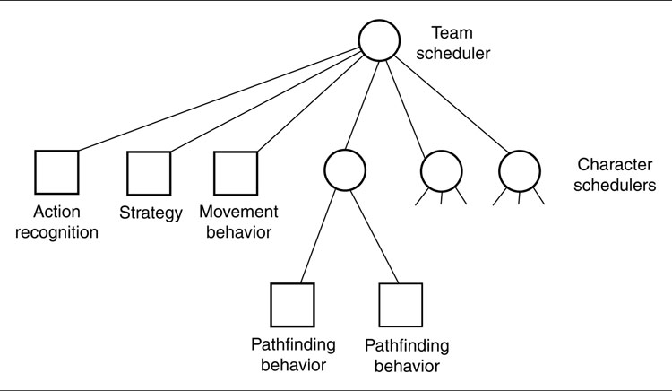
Figure 6.26: A hierarchical scheduling system for multi-tier AI
So far we’ve looked at cooperation mechanics where individual characters obey some kind of guiding control. The control might be the player’s explicit orders, a tactical decision making tool, or any other decision maker operating on behalf of the whole group.
This is a powerful technique that naturally fits in with the way we think about the goals of a group and the orders that carry them out. It has the weakness, however, of relying on the quality of the high-level decision. If a character cannot obey the higher level decision for some reason, then it is left without any ability to make progress.
We could instead use less centralized techniques to make a number of characters appear to be working together. They do not need to coordinate in the same way as for multi-tier AI, but by taking into account what each other is doing, they can appear to act as a coherent whole. This is the approach taken in most squad-based games.
Each character has its own decision making, but the decision making takes into account what other characters are doing. This may be as simple as moving toward other characters (which has the effect that characters appear to stick together), or it could be more complex, such as choosing another character to protect and maneuvering to keep them covered at all times.

Figure 6.27: State machines for emergent fire team behavior
Figure 6.27 shows an example finite state machine for four characters in a fire team. Four characters with this finite state machine will act as a team, providing mutual cover and appearing to be a coherent whole. There is no higher level guidance being provided.
If any member of the team is removed, the rest of the team will still behave relatively efficiently, keeping themselves safe and providing offensive capability when needed.
We could extend this and produce different state machines for each character, adding their team specialty: the grenadier could be selected to fire on an enemy behind light cover, a designated medic could act on fallen comrades, and the radio operator could call in air strikes against heavy opposition. All this could be achieved through individual state machines.
Scalability
As you add more characters to an emergently cooperating group, you will reach a threshold of complexity. Beyond this point it will be difficult to control the behavior of the group. The exact point where this occurs depends on the complexity of the behaviors of each individual.
Reynolds’s flocking algorithm, for example, can scale to hundreds of individuals with only minor tweaks to the algorithm. The fire team behaviors earlier in the section are fine up to six or seven characters, whereupon they become less useful. The scalability seems to depend on the number of different behaviors each character can display. As long as all the behaviors are relatively stable (such as in the flocking algorithm), the whole group can settle into a reasonable stable behavior, even if it appears to be highly complex. When each character can switch to different modes (as in the finite state machine example), we end up rapidly getting into oscillations.
Problems occur when one character changes behavior which forces another character to also change behavior and then a third, which then changes the behavior of the first character again, and so on. Some level of hysteresis in the decision making can help (i.e., a character keeps doing what it has been doing for a while, even if the circumstances change), but it only buys us a little time and cannot solve the problem.
To solve this issue we have two choices. First, we can simplify the rules that each character is following. This is appropriate for games with a lot of identical characters. If, in a shooter, we are up against 1,000 enemies, then it makes sense that they are each fairly simple and that the challenge arises from their number rather than their individual intelligence. On the other hand, if we are facing scalability problems before we get into double-digit numbers of characters, then this is a more significant problem.
The best solution is to set up a multi-tiered AI with different levels of emergent behavior. We could have a set of rules very similar to the state machine example, where each individual is a whole squad rather than a single character. Then in each squad the characters can respond to the orders given from the emergent level, either directly obeying the order or including it as part of their decision making process for a more emergent and adaptive feel.
This is something of a cheat, of course, if the aim is to be purely emergent. But if the aim is to get great AI that is dynamic and challenging (which, let’s face it, it should be), then it is often an excellent compromise.
In my experience many developers who have tried to implement emergent behaviors have struck scalability problems quickly and ended up with some variation of this more practical approach.
Predictability
A side effect of this kind of emergent behavior is that you often get group dynamics that you didn’t explicitly design. This is a double-edged sword; it can be beneficial to see emergent intelligence in the group, but this doesn’t happen very often (don’t believe the hype you read about this stuff). The most likely outcome is that the group starts to do something really annoying that looks unintelligent. It can be very difficult to eradicate these dynamics by tweaking the individual character behaviors.
It is almost impossible to work out how to create individual behaviors that will emerge into exactly the kind of group behavior you are looking for. In my experience the best you can hope for is to try variations until you get a group behavior that is reasonable and then tweak that. This may be exactly what you want.
If you are looking for highly intelligent high-level behavior, then you will always end up implementing it explicitly. Emergent behavior is useful and can be fun to implement, but it is certainly not a way of getting great AI with less effort.

Figure 6.28: An action sequence needing timing data
Making sure that all the members of a group work together is difficult to do from first principles. A powerful tool is to use a script that shows what actions need to be applied in what order and by which character. In Chapter 5 we looked at action execution and scripted actions as a sequence of primitive actions that can be executed one after another.
We can extend this to groups of characters, having a script per character. Unlike for a single character, however, there are timing complications that make it difficult to keep the illusion of cooperation among several characters. Figure 6.28 shows a situation in football where two characters need to cooperate to score a touchdown. If we use the simple action script shown, then the overall action will be a success in the first instance, but a failure in the second instance.
To make cooperative scripts workable, we need to add the notion of interdependence of scripts. The actions that one character is carrying out need to be synchronized with the actions of other characters.
We can achieve this most simply by using signals. In place of an action in the sequence, we allow two new kinds of entity: signal and wait.
Signal: A signal has an identifier. It is a message sent to anyone else who is interested. This is typically any other AI behavior, although it could also be sent through an event or sense simulation mechanism from Chapter 11 if finer control is needed.
Wait: A wait also has an identifier. It stops any elements of the script from progressing unless it receives a matching signal.
We could go further and add additional programming language constructs, such as branches, loops, and calculations. This would give us a scripting language capable of any kind of logic, but at the cost of significantly increased implementation difficulty and a much bigger burden on the content creators who have to create the scripts.
Adding just signals and waits allows us to use simple action sequences for collaborative actions between multiple characters.
In addition to these synchronization elements, some games also admit actions that need more than one character to participate. Two soldiers in a squad-based shooter might be needed to climb over a wall: one to climb and the other to provide a leg-up. In these cases some of the actions in the sequence may be shared between multiple characters. The timing can be handled using waits, but the actions are usually specially marked so each character is aware that it is performing the action together, rather than independently.
Adding in the elements from Chapter 5, a collaborative action sequencer supports the following primitives:
State Change Action: This is an action that changes some piece of game state without requiring any specific activity from any character.
Animation Action: This is an action that plays an animation on the character and updates the game state. This is usually independent of other actions in the game. This is often the only kind of action that can be performed by more than one character at the same time. This can be implemented using unique identifiers, so different characters can understand when they need to perform an action together and when they only need to perform the same action at the same time.
AI Action: This is an action that runs some other piece of AI. This is often a movement action, which gets the character to adopt a particular steering behavior. This behavior can be parameterized—for example, an arrive behavior having its target set. It might also be used to get the character to look for firing targets or to plan a route to its goal.
Compound Action: This takes a group of actions and performs them at the same time.
Action Sequence: This takes a group of actions and performs them in series.
Signal: This sends a signal to other characters.
Wait: This waits for a signal from other characters.
The implementation of the first five types were discussed in Chapter 5, including pseudo-code for compound actions and action sequences. To make the action execution system support synchronized actions, we need to implement signals and waits.
Pseudo-Code
The wait action can be implemented in the following way:

Note that we don’t want the character to freeze while waiting. We have added a waiting action to the class, which is carried out while the character waits.
A signal implementation is even simpler. It can be implemented in the following way:

Data Structures and Interfaces
This code assumes that there is a central store of signal identifiers that can be checked against, called globalIdStore. This can be a simple hash set, but should probably be emptied of stale identifiers from time to time. It has the following interface:
Implementation Notes
Another complication with this approach is the confusion between different occurrences of a signal. If a set of characters perform the same script more than once, then there will be an existing signal in the store from the previous time through. This may mean that none of the waits actually waits.
For that reason it is wise to have a script remove all the signals it intends to use from the global store before it runs. If there is more than one copy of a script running simultaneously (e.g., if two squads are both performing the same set of actions at different locations), then the identifier will need to be disambiguated further. If this situation could arise in your game, it may be worth moving to a more fine-grained messaging technique among each squad, such as the message passing algorithm in Chapter 11. Each squad then communicates signals only with others in the squad, removing all ambiguity.
Performance
Both the signal and wait actions are O(1) in both time and memory. In the implementation above, the Wait class needs to access the IdStore interface to check for signals. If the store is a hash set (which is its most likely implementation), then this will be an
Although the wait action can cause the action manager to stop processing any further actions, the algorithm will return in constant time each frame (assuming the wait action is the only one being processed).
Creating Scripts
The infrastructure to run scripts is only half of the implementation task. In a full engine we need some mechanism to allow level designers or character designers to create the scripts.
This can be achieved using a simple text file with primitives that represent each kind of action, signal, and wait. Chapter 13, Section 13.3 gives some high-level information about how to create a parser to read and interpret text files of data. Alternatively, a tool can be exposed in the game engine editor to allow designers to build scripts out of visual components. Chapter 12 has more information about incorporating AI editors into the game production toolchain.
The next section on military tactics provides an example set of scripts for a collaborative action used in a real game scenario.
So far we have looked at general approaches for implementing tactical or strategic AI. Most of the technology requirements can be fulfilled using common-sense applications of the techniques we’ve looked at throughout the book. To those, we add the specific tactical reasoning algorithms to get a better idea of the overall situation facing a group of characters.
As with all game development, we need both the technology to support a behavior and the content for the behavior itself. Although this will dramatically vary depending on the genre of game and the way the character is implemented, there are resources available for tactical behaviors of a military unit.
In particular, there is a large body of freely available information on specific tactics used by both the U.S. military and other NATO countries. This information is made up of training manuals intended for use by regular forces.
The U.S. infantry training manuals, in particular, can be a valuable resource for implementing military-style tactics in any genre of game from historical World War II games through to far future science fiction or medieval fantasy. They contain information for the sequences of events needed to accomplish a wide range of objectives, including military operations in urban terrain (MOUT), moving through wilderness areas, sniping, relationships with heavy weapons, clearing a room or a building, and setting up defensive camps.
I have found that this kind of information is most suited to a cooperation script approach, rather than open-ended multi-tier or emergent AI. A set of scripts can be created that represents the individual stages of the operation, and these can then be made into a higher level script that coordinates the lower level events. As in all scripted behaviors, some feedback is needed to make sure the behaviors remain sensible throughout the script execution. The end result can be deeply uncanny: seeing characters move as a well-oiled fighting team and performing complex series of inter-timed actions to achieve their goal.
As an example of the kinds of script needed in a typical situation, let’s look at implementations for an indoor squad-based shooter.
Case Study: A Fire Team Takes a House
Let’s say that we have a game with a modern military setting where the AI team is a squad of special forces soldiers specializing in anti-terrorism duties. Their aim is to take a house rapidly and with extreme aggression to make sure the threat from its occupants is neutralized as fast as possible. In this simulation the player is not a member of the team but was a controlling operator scheduling the activities of several such special forces units.
The source material for this project was the “U.S. Army Field Manual 3-06.11 Combined Arms Operations in Urban Terrain” [72]. This particular manual contains step-by-step diagrams for moving along corridors, clearing rooms, moving across junctions, and general combat indoors.
Figure 6.29 shows the sequence for room clearing. First, the team assembles in set format outside the doorway. Second, a grenade is thrown into the room (this will be a stun grenade if the room might contain non-combatants or a lethal grenade otherwise). The first soldier into the room moves along the near wall and takes up a location in the corner, covering the room. The second soldier does the same to the adjacent corner. The remaining soldiers cover the center of the room. Each soldier shoots at any target they can see during this movement.
The game uses four scripts:
• Move into position outside the door.
• Throw in a grenade.
• Move into a corner of the room.
• Flank the inside of the doorway.
A top-level script coordinates these actions in turn. This script needs to first calculate the two corners required for the clearance. These are the two corners closest to the door, excluding corners that are too close to the door to allow a defensive position to be occupied. In the implementation for this game, a waypoint tactics system had already been used to identify all the corners in all the rooms in the game, along with waypoints for the door and locations on either side of the door both inside and out.

Figure 6.29: Taking a room
Determining the nearest corners in this way allows for the same script to be used on buildings of all different shapes, as shown in Figure 6.30.
The interactions between the scripts (using the Signal and Wait instances we saw earlier) allow the team to wait for the grenade to explode and to move in a coordinated way to their target locations while maintaining cover over all of the room.
A different top-level script is used for two- and three-person room clearances (in the case that one or more team members are eliminated), although the lower level scripts are identical in each case. In the three-person script, there is only one person left by the door (the first two still take the corners). In the two-person script, only the corners are occupied, and the door is left.

Figure 6.30: Taking various rooms
EXERCISES
6.1 Figure 6.31 shows a map with some unlabeled tactical points. Label points that would provide cover, points that are exposed, points that would make good ambush points, etc.
6.2 On page 492 suppose that, instead of interpreting the given waypoint values as degrees of membership, we interpret them as probabilities. Then, assuming cover and visibility values are independent, what is the probability that the location is a good sniping location?
6.3 Figure 6.32 shows a map with some cover points.Pre-determine the directions of cover and then compare the results to a post-processing step that uses line-of-sight tests to the indicated enemies.
6.4 Design a state machine that would produce behavior similar to that of the decision tree from Figure 6.6.

Figure 6.31: Tactical points in part of a game level
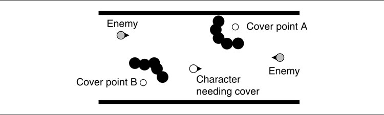
Figure 6.32: Cover points in part of a game level
6.5 Using the map from Exercise 6.3 calculate the runtime cover quality of the two potential cover points. Why might it be more reliable to try testing with some random offsets around cover point B?
6.6 Suppose that in Figure 6.9 the values of the waypoints are A, 1.7; B, 2.3; and C, 1.1. What is the result of applying the condensation algorithm? Is the result desirable?
6.7 Convolve the following filter with the 3 × 3 section of the map that appeared in Section 6.2.7.
What does the filter do? Why might it be useful? What problem can occur at the edges and how can it be fixed?

Figure 6.33: Military forces in a grid-based level
6.8 Use a linear influence drop-off to calculate the influence map for the placement of military forces in Figure 6.33.If you are doing this exercise by hand, for simplicity, use the Manhattan distance to calculate all distances and assume a maximum radius of influence of 4. If you are writing code, then experiment with different settings for distance, influence drop-off, and maximum radius.
6.9 Use the influence map you calculated in Exercise 6.8 to determine the security level. Identify an area on the border where Black might consider an attack.
6.10 If in Exercise 6.9 we only had to calculate the security level at the border, what (if any) military units could we safely ignore and why?
6.11 Repeat Exercise 6.9, but this time calculate the security level from White’s point of view assuming White doesn’t know about Black’s military unit of strength 2.
6.12 Suppose White uses the answer from 6.11 to mount an attack that moves from right to left along the bottom of the grid, then how might a frag-map help to infer the existence of an unknown enemy unit?
6.13 If Black knew that White had incorrect information such as in 6.11, how could Black use it to their advantage? In particular, devise a scheme to determine the best placement of a hidden unit by calculating the quality of a cell based on the cover it provides (better cover increases the chance of the unit remaining hidden), the actual security of the cell, and the (incorrect) perceived security from the enemy’s point of view.
6.14 Using the map from Exercise 6.8, calculate the influence map by using the same 3 × 3 convolution filter given at the start of Section 6.2.7. You might want to use a computer to help you answer this question.
1. Convolution filters are strictly only one technique used in finite element simulation.
2. These are literally unpredictable: in the sense that the only way to find out what will happen is to run the cellular automaton.