GAME CHARACTERS usually need to move around their level. Sometimes this movement is set in stone by the developers, such as a patrol route that a guard can follow blindly or a small fenced region in which a dog can randomly wander around. Fixed routes are simple to implement, but can easily be fooled if an object is pushed in the way. Free wandering characters can appear aimless and can easily get stuck.
More complex characters don’t know in advance where they’ll need to move. A unit in a real-time strategy game may be ordered to any point on the map by the player at any time, a patrolling guard in a stealth game may need to move to its nearest alarm point to call for reinforcements, and a platform game may require opponents to chase the player across a chasm using available platforms.
For each of these characters the AI must be able to calculate a suitable route through the game level to get from where it is now to its goal. We’d like the route to be sensible and as short or rapid as possible (it doesn’t look smart if your character walks from the kitchen to the lounge via the attic).
This is pathfinding, sometimes called path planning, and it is everywhere in game AI.
In our model of game AI (Figure 4.1), pathfinding sits on the border between decision making and movement. Often, it is used simply to work out where to move to reach a goal; the goal is decided by another bit of AI, and the pathfinder simply works out how to get there. To accomplish this, it can be embedded in a movement control system so that it is only called when it is needed to plan a route. This is discussed in Chapter 3 on movement algorithms.
But pathfinding can also be placed in the driving seat, making decisions about where to move as well as how to get there. I’ll look at a variation of pathfinding, open goal pathfinding, that can be used to work out both the path and the destination.
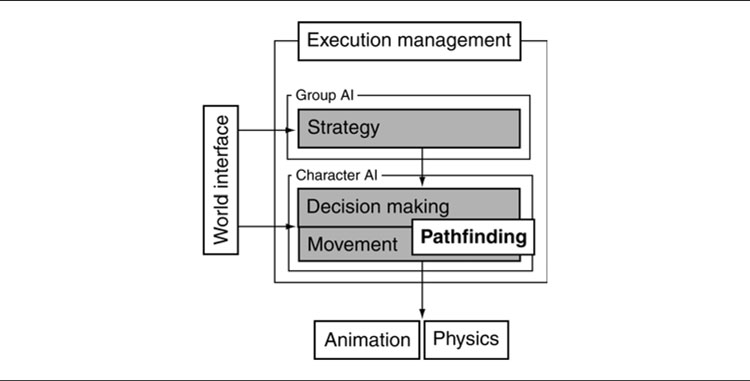
Figure 4.1: The AI model
The vast majority of games use pathfinding solutions based on an algorithm called A*. Although it’s efficient and easy to implement, A* can’t work directly with the game level data. It requires that the game level be represented in a particular data structure: a directed nonnegative weighted graph.
This chapter introduces the graph data structure and then looks at the older brother of the A* algorithm, the Dijkstra algorithm. Although Dijkstra is more often used in tactical decision making than in pathfinding, it is a simpler version of A*, so we’ll cover it here on the way to the full A* algorithm.
Because the graph data structure isn’t the way that most games would naturally represent their level data, we’ll look in some detail at the knowledge representation issues involved in turning the level geometry into pathfinding data. Finally, we’ll look at a handful of the many tens of useful variations of the basic A* algorithm.
Neither A* nor Dijkstra (nor their many variations) can work directly on the geometry that makes up a game level. They rely on a simplified version of the level represented in the form of a graph. If the simplification is done well (and we’ll look at how later in the chapter), then the plan returned by the pathfinder will be useful when translated back into game terms. On the other hand, in the simplification we throw away information, and that might be significant information. Poor simplification can mean that the final path isn’t so good.
Pathfinding algorithms use a type of graph called a directed non-negative weighted graph. I’ll work up to a description of the full pathfinding graph via simpler graph structures.

Figure 4.2: A general graph
A graph is a mathematical structure often represented diagrammatically. It has nothing to do with the more common use of the word “graph” to mean any diagram, such as a pie chart or histogram.
A graph consists of two different types of element: nodes are often drawn as points or circles in a graph diagram, while connections link nodes together with lines (as we’ll see below, both of these elements are called various different names by different people). Figure 4.2 shows a graph structure.
Formally, the graph consists of a set of nodes and a set of connections, where a connection is simply an unordered pair of nodes (the nodes on either end of the connection).
For pathfinding, each node usually represents a region of the game level, such as a room, a section of corridor, a platform, or a small region of outdoor space. Connections show which locations are connected. If a room adjoins a corridor, then the node representing the room will have a connection to the node representing the corridor. In this way the whole game level is split into regions, which are connected together. Later in the chapter, we’ll see a way of representing the game level as a graph that doesn’t follow this model, but in most cases this is the approach taken.
To get from one location in the level to another, we use connections. If we can go directly from our starting node to our target node, then our task is simple: we use the connection. Otherwise, we may have to use multiple connections and travel through intermediate nodes on the way.
A path through the graph consists of zero or more connections. If the start and end node are the same, then there are no connections in the path. If the nodes are connected, then only one connection is needed, and so on.

Figure 4.3: A weighted graph
A weighted graph is made up of nodes and connections, just like the general graph. In addition to a pair of nodes for each connection, we add a numerical value. In mathematical graph theory this is called the weight, and in game applications it is more commonly called the cost (although the graph is still called a “weighted graph” rather than a “costed graph”).
In the example graph shown in Figure 4.3, we see that each connection is labeled with an associated cost value.
The costs in a pathfinding graph often represent time or distance. If a node representing one end of a corridor is a long distance from the node representing the other, then the cost of the connection will be large. Similarly, moving between two areas with difficult terrain will take a long time, so the cost will be large.
The costs in a graph can represent more than just time or distance. They might represent strategic risk or loot availability, for example. We will see a number of applications of pathfinding to situations where the cost is a combination of time, distance, and other factors.
For a whole route through a graph, from a start node to a target node, we can work out the total path cost. It is simply the sum of the costs of each connection in the route. In Figure 4.4,if we are heading from node A to node C, via node B, and if the costs are 4 from A to B and 5 from B to C, then the total cost of the route is 9.

Figure 4.4: Total path cost from A to C is 4 + 5 = 9
Representative Points in a Region
You might notice immediately that if two regions are connected (such as a room and a corridor), then the distance between them (and therefore the time to move between them) will be zero. If you are standing in a doorway, then moving from the room side of the doorway to the corridor side is instant. So shouldn’t all connections have a zero cost?
We tend to measure connection distances or times from a representative point in each region. So we pick the center of the room and the center of the corridor. If the room is large and the corridor is long, then there is likely to be a large distance between their center points, so the cost will be large.
You will often see this in diagrams of pathfinding graphs, such as Figure 4.5: a representative point is marked in each region.
A complete analysis of this approach will be left to a later section. It is one of the subtleties of representing the game level for the pathfinder, and we’ll return to the issues it causes at some length.
The Non-Negative Constraint
It doesn’t seem to make sense to have negative costs. You can’t have a negative distance between two points, and it can’t take a negative amount of time to move there.
Mathematical graph theory does allow negative weights, however, and they have direct applications in some practical problems. These problems are entirely outside of normal game development, and all of them are beyond the scope of this book. Writing algorithms that can work with negative weights is typically more complex than for those with strictly non-negative weights.

Figure 4.5: Weighted graph overlaid onto level geometry
In particular, the Dijkstra and A* algorithms should only be used with non-negative weights. It is possible to construct a graph with negative weights such that a pathfinding algorithm will return a sensible result. In the majority of cases, however, Dijkstra and A* would go into an infinite loop. This is not an error in the algorithms. Mathematically, there is no such thing as a shortest path across many graphs with negative weights; a solution simply doesn’t exist.
When I use the term “cost” in this book, it means a non-negative weight. Costs are always positive. We will never need to use negative weights or the algorithms that can cope with them. I’ve never needed to use them in any game development project I’ve worked on, and I can’t foresee a situation when I might.
4.1.3 DIRECTED WEIGHTED GRAPHS
For many situations a weighted graph is sufficient to represent a game level, and I have seen implementations that use this format. We can go one stage further, however. The major pathfinding algorithms support the use of a more complex form of graph, the directed graph (see Figure 4.6), which is often useful to developers.
So far we’ve assumed that if it is possible to move between node A and node B (the room and corridor, for example), then it is possible to move from node B to node A. Connections go both ways, and the cost is the same in both directions. Directed graphs instead assume that connections are in one direction only. If you can get from node A to node B, and vice versa, then there will be two connections in the graph: one for A to B and one for B to A.
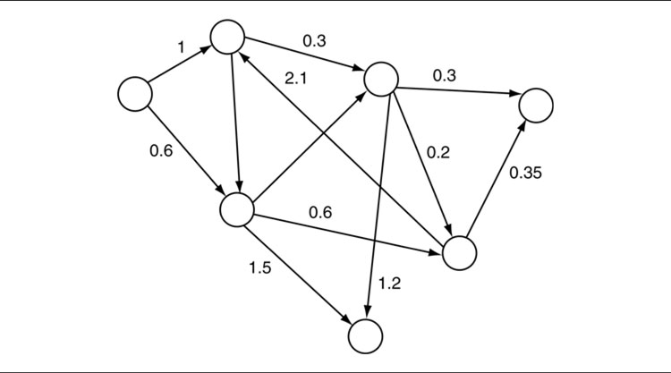
Figure 4.6: A directed weighted graph
This is useful in many situations. First, it is not always the case that the ability to move from A to B implies that B is reachable from A. If node A represents an elevated walkway and node B represents the floor of the warehouse underneath it, then a character can easily drop from A to B but will not be able to jump back up again.
Second, having two connections in different directions means that there can be two different costs. Let’s take the walkway example again but add a ladder. Thinking about costs in terms of time, it takes almost no time at all to fall off the walkway, but it may take several seconds to climb back up the ladder. Because costs are associated with each connection, this can be simply represented: the connection from A (the walkway) to B (the floor) has a small cost, and the connection from B to A has a larger cost.
Mathematically, a directed graph is identical to a non-directed graph, except that the pair of nodes that makes up a connection is now ordered. Whereas a connection <node A, node B, cost> in a non-directed graph is identical to <node B, node A, cost> (so long as the costs are equal), in a directed graph they are different connections.
Terminology for graphs varies. In mathematical texts you often see vertices rather than nodes and edges rather than connections (and, as we’ve already seen, weights rather than costs). Many AI developers who actively research pathfinding use this terminology from exposure to the mathematical literature. It can be confusing in a game development context because vertices more commonly refer to a component of 3D geometry, something altogether different.
There is no agreed terminology for pathfinding graphs in games articles and seminars. I have seen locations and even “dots” for nodes, and I have seen arcs, paths, links, and “lines” for connections.
I will use the nodes and connections terminology throughout this chapter because it is common, relatively meaningful (unlike dots and lines), and unambiguous (arcs and vertices both have meaning in game graphics).
In addition, while I have talked about directed non-negative weighted graphs, almost all pathfinding literature just calls them graphs and assumes that you know what kind of graph is meant. I will do the same.
We need to represent our graph in such a way that pathfinding algorithms such as A* and Dijkstra can work with it.
As we will see, the algorithms need to query the outgoing connections from any given node. And for each such connection, they need to have access to its cost and destination.
We can represent the graph to our algorithms using the following interface:

The graph class simply returns an array of connection objects for any node that is queried. From these objects the end node and cost can be retrieved.
A simple implementation of this class would store the connections for each node and simply return the list. Each connection would have the cost and end node stored in memory.
A more complex implementation might calculate the cost only when it is required, using information from the current structure of the game level.
Notice that there is no interface for a Node in this listing, because we don’t need to specify one. In many cases it is sufficient just to give nodes a unique number and to use integers as the data type. In fact, we will see that this is a particularly powerful implementation because it opens up some specific, very fast optimizations of the A* algorithm.
The Dijkstra algorithm is named for Edsger Dijkstra, the mathematician who devised it (and the same man who coined the famous programming phrase “GOTO considered harmful”).
Dijkstra’s algorithm [10] wasn’t originally designed for pathfinding as games understand it. It was designed to solve a problem in mathematical graph theory, confusingly called “shortest path.”
Where pathfinding in games has one start point and one goal point, the shortest path algorithm is designed to find the shortest routes to everywhere from an initial point. The solution to this problem will include a solution to the pathfinding problem (we’ve found the shortest route to everywhere, after all), but it is wasteful if we are going to throw away all the other routes. It can be modified to generate only the path we are interested in, but is still quite inefficient at doing that.
Because of these issues, Dijkstra is rarely used in production pathfinding. And to my knowledge never as the main pathfinding algorithm. Nonetheless, it is an important algorithm for tactical analysis (covered in Chapter 6, Tactical and Strategic AI) and has uses in a handful of other areas of game AI.
I will introduce it here rather than in that chapter, because it is a simpler version of the main pathfinding algorithm A*, and understanding Dijkstra enough to implement it is a good step to understanding and implementing A*.
Given a graph (a directed non-negative weighted graph) and two nodes (called start and goal) in that graph, we would like to generate a path from start to goal such that the total path cost of that path is minimal, i.e. there should be no lower cost paths from start to goal.
There may be any number of paths with the same minimal cost. Figure 4.7 has 10 possible paths, all with the same minimal cost. When there is more than one optimal path, we only expect one to be returned, and we don’t care which one it is.
Recall that the path we expect to be returned consists of a set of connections, not nodes. Two nodes may be linked by more than one connection, and each connection may have a different cost (it may be possible to either fall off a walkway or climb down a ladder, for example). We therefore need to know which connections to use; a list of nodes will not suffice.
Many games don’t make this distinction. There is, at most, one connection between any pair of nodes. After all, if there are two connections between a pair of nodes, the pathfinder should always take the one with the lower cost. In some applications, however, the costs change over the course of the game or between different characters, and keeping track of multiple connections is useful.

Figure 4.7: All optimal paths
There is no more work in the algorithm to cope with multiple connections. And for those applications where it is significant, it is often essential. For those reasons, I will always assume a path consists of connections.
Informally, Dijkstra works by considering paths that spread out from the start node along its connections. As it spreads out to more distant nodes, it keeps a record of the direction it came from (imagine it drawing chalk arrows on the floor to indicate the way back to the start). Eventually, one of these paths will reach the goal node and the algorithm can follow the chalk arrows back to its start point to generate the complete route. Because of the way Dijkstra regulates the spreading process, it guarantees that the first valid path it finds will also be the cheapest (or one of the cheapest if there are more with the same lowest cost). This valid path is found as soon as the algorithm considers the goal node. The chalk arrows always point back along the shortest route to the start.
Let’s break this down in more detail.
Dijkstra works in iterations. At each iteration it considers one node of the graph and follows its outgoing connections, storing the node at the other end of those connections in a pending list. When the algorithm begins only the start node is placed in this list, so at the first iteration it considers the start node. At successive iterations it chooses a node from the list using an algorithm I’ll describe shortly. I’ll call each iteration’s node the “current node.” When the current node is the goal, the algorithm is done. If the list is ever emptied, we know that goal cannot be reached.

Figure 4.8: Dijkstra at the first node
Processing the Current Node
During an iteration, Dijkstra considers each outgoing connection from the current node. For each connection it finds the end node and stores the total cost of the path so far (we’ll call this the “cost-so-far”), along with the connection it arrived there from.
In the first iteration, where the start node is the current node, the total cost-so-far for each connection’s end node is simply the cost of the connection. Figure 4.8 shows the situation after the first iteration. Each node connected to the start node has a cost-so-far equal to the cost of the connection that led there, as well as a record of which connection that was.
For iterations after the first, the cost-so-far for the end node of each connection is the sum of the connection cost and the cost-so-far of the current node (i.e., the node from which the connection originated). Figure 4.9 shows another iteration of the same graph. Here the cost-so-far stored in node E is the sum of cost-so-far from node B and the connection cost of Connection IV from B to E.
In implementations of the algorithm, there is no distinction between the first and successive iterations. By setting the cost-so-far value of the start node as 0 (since the start node is at zero distance from itself), we can use one piece of code for all iterations.
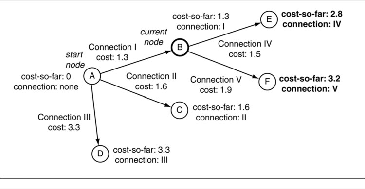
Figure 4.9: Dijkstra with a couple of nodes
The Node Lists
The algorithm keeps track of all the nodes it has seen so far in two lists: open and closed. In the open list it records all the nodes it has seen, but that haven’t had their own iteration yet. It also keeps track of those nodes that have been processed in the closed list. To start with, the open list contains only the start node (with zero cost-so-far), and the closed list is empty.
Each node can be thought of as being in one of three categories: it can be in the closed list, having been processed in its own iteration; it can be in the open list, having been visited from another node, but not yet processed in its own right; or it can be in neither list. The node is sometimes said to be closed, open, or unvisited.
At each iteration, the algorithm chooses the node from the open list that has the smallest cost-so-far. This is then processed in the normal way. The processed node is then removed from the open list and placed on the closed list.
There is one complication. When we follow a connection from the current node, we’ve assumed that we’ll end up at an unvisited node. We may instead end up at a node that is either open or closed, and we’ll have to deal slightly differently with them.
Calculating Cost-So-Far for Open and Closed Nodes
If we arrive at an open or closed node during an iteration, then the node will already have a cost-so-far value and a record of the connection that led there. Simply setting these values will overwrite the previous work the algorithm has done.
Instead, we check if the route we’ve now found is better than the route that we’ve already found. Calculate the cost-so-far value as normal, and if it is higher than the recorded value (and it will be higher in almost all cases), then don’t update the node at all and don’t change what list it is on.

Figure 4.10: Open node update
If the new cost-so-far value is smaller than the node’s current cost-so-far, then update it with the better value, and set its connection record. The node should then be placed on the open list. If it was previously on the closed list, it should be removed from there.
Strictly speaking, Dijkstra will never find a better route to a closed node, so we could check if the node is closed first and not bother doing the cost-so-far check. A dedicated Dijkstra implementation would do this. We will see that the same is not true of the A* algorithm, however, and we will have to check for faster routes in both cases.
Figure 4.10 shows the updating of an open node in a graph. The new route, via node C, is faster, and so the record for node D is updated accordingly.
Terminating the Algorithm
The basic Dijkstra algorithm terminates when the open list is empty: it has considered every node in the graph that be reached from the start node, and they are all on the closed list.
For pathfinding, we are only interested in reaching the goal node, however, so we can stop earlier. The algorithm should terminate when the goal node is the smallest node on the open list.
Notice that this means we will have already reached the goal on a previous iteration, when it was placed into the open list. Why not simply terminate the algorithm as soon as we’ve found the goal?

Figure 4.11: Following the connections to get a plan
Consider Figure 4.10 again. If D is the goal node, then we’ll first find it when we’re processing node B. So if we stop here, we’ll get the route A–B–D, which is not the shortest route. To make sure there can be no shorter routes, we have to wait until the goal has the smallest cost-so-far. At this point, and only then, we know that a route via any other unprocessed node (either open or unvisited) must be longer.
This rule is often broken, and many developers implement their pathfinding algorithms to terminate as soon as the goal node is seen, rather than waiting for it to be selected from the open list. Whether this is done intentionally or because of a mistake in the implementation, in practice it is barely noticeable. The first route found to the goal is very often the shortest, and even when there is a shorter route, it is usually only a tiny amount longer.
Retrieving the Path
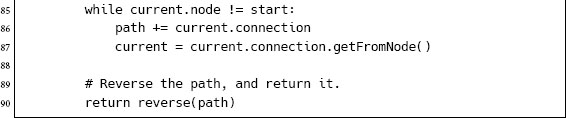
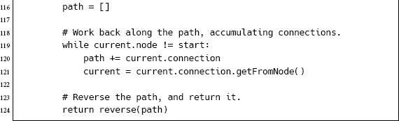
The final stage is to retrieve the path.
We do this by starting at the goal node and looking at the connection that was used to arrive there. We then go back and look at the start node of that connection and do the same. We continue this process, keeping track of the connections, until the original start node is reached. The list of connections is correct, but in the wrong order, so we reverse it and return the list as our solution.
Figure 4.11 shows a simple graph after the algorithm has run. The list of connections found by following the records back from the goal is reversed to give the complete path.
The Dijkstra pathfinder takes as input a graph (conforming to the interface given in the previous section), a start node, and an end node. It returns an array of connection objects that represent a path from the start node to the end node.


Other Functions
The pathfinding list is a specialized data structure that acts very much like a regular list. It holds a set of NodeRecord structures and supports the following additional methods:
• The smallestElement method returns the NodeRecord structure in the list with the lowest costSoFar value.
• The contains(node) method returns true only if the list contains a NodeRecord structure whose node member is equal to the given parameter.
• The find(node) method returns the NodeRecord structure from the list whose node member is equal to the given parameter.
In addition, I have used a function, reverse(array), that returns a reversed copy of a normal array.
4.2.4 DATA STRUCTURES AND INTERFACES
There are three data structures used in the algorithm: the simple list used to accumulate the final path, the pathfinding list used to hold the open and closed lists, and the graph used to find connections from a node (and their costs).
Simple List
The simple list is not very performance critical, since it is only used at the end of the pathfinding process. It can be implemented as a basic linked list (a std::list in C++, for example) or even a resizable array (such as std::vector in C++).
Pathfinding List
The open and closed lists in the Dijkstra algorithm (and in A*) are critical data structures that directly affect the performance of the algorithm. A lot of the optimization effort in pathfinding goes into their implementation. In particular, there are four operations on the list that are critical:
1. Adding an entry to the list (the +=operator);
2. Removing an entry from the list (the -= operator);
3. Finding the smallest element (the smallestElement method);
4. Finding an entry in the list corresponding to a particular node (the contains and find methods both do this).
Finding a suitable balance between these four operations is key to building a fast implementation. Unfortunately, the balance is not always identical from game to game.
Because the pathfinding list is most commonly used with A* for pathfinding, a number of its optimizations are specific to that algorithm. I will wait to describe it in more detail until we have looked at A*.
Graph
We have seen the interface presented by the graph in the first section of this chapter.
The getConnections method is called low down in the loop and is typically a critical performance element to get right. The most common implementation has a lookup table indexed by a node (where nodes are numbered as consecutive integers). The entry in the lookup table is an array of connection objects. Thus, the getConnections method needs to do minimal processing and is efficient.
Some methods of translating a game level into a pathfinding graph do not allow for this simple lookup approach and can therefore lead to much slower pathfinding. Such situations are described in more detail later in the chapter, in Section 4.4 on world representation.
The getToNode and getCost methods of the Connection class are even more performance critical. In an overwhelming majority of implementations, however, no processing is performed in these methods, and they simply return a stored value in each case. The Connection class might therefore look like the following:
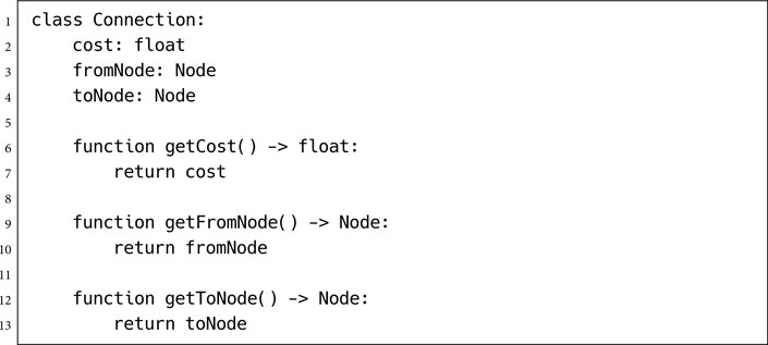
For this reason the Connection class is rarely a performance bottleneck.
Of course, these values need to be calculated somewhere. This is usually done when the game level is converted into a graph and is an offline process independent of the pathfinder.
The practical performance of Dijkstra in both memory and speed depends mostly on the performance of the operations in the pathfinding list data structure.
Ignoring the performance of the data structure for a moment, we can see the theoretical performance of the overall algorithm. The algorithm considers each node in the graph that is closer than the end node. Call this number n. For each of these nodes, it processes the inner loop once for each outgoing connection. Call the average number of outgoing connections per node m. So the algorithm itself is O(nm) in execution speed. The total memory use depends on both the size of the open list and the size of the closed list. When the algorithm terminates there will be n elements in the closed list and no more than nm elements in the open list (in fact, there will typically be fewer than n elements in the open list). So the worst case memory use is O(nm).
To include the data structure times, we note that both the list addition and the find operation (see the section on the pathfinding list data structure, above) are called nm times, while the extraction and smallestElement operations are called n times. If the order of the execution time for the addition or find operations is greater than O(m), or if the extraction and smallestElement operations are greater than O(1), then the actual execution performance will be worse than O(nm).
In order to speed up the key operations, data structure implementations are often chosen that have worse than O(nm) memory requirements.
When we look in more depth at the list implementations in the next section, we will consider their impact on performance characteristics.
If you look up Dijkstra in a computer science textbook, it may tell you that it is O(n2). In fact, this is exactly the result above. The worst conceivable performance occurs when the graph is so densely connected that m≈ n. This is almost never the case for the graphs that represent game levels: the number of connections per node stays roughly constant no matter how many nodes the level contains, so citing the performance as O(n2) would be misleading. Alternatively, the performance may be given as O(m + n log n) in time, which is the performance of the algorithm when using a ‘Fibonacci heap’ data structure for the node lists [57].
The principle problem with Dijkstra is that it searches the entire graph indiscriminately for the shortest possible route. This is useful if we’re trying to find the shortest path to every possible node (the problem that Dijkstra was designed for), but wasteful for point-to-point pathfinding.
We can visualize the way the algorithm works by showing the nodes currently on its open and closed lists at various stages through a typical run. This is shown in Figure 4.12.
In each case the boundary of the search is made up of nodes on the open list. This is because the nodes closer to the start (i.e., with lower distance values) have already been processed and placed on the closed list.

Figure 4.12: Dijkstra in steps
The final part of Figure 4.12 shows the state of the lists when the algorithm terminates. The line shows the best path that has been calculated. Notice that most of the level has still been explored, even well away from the path that is generated.
The number of nodes that were considered, but never made part of the final route, is called the fill of the algorithm. In general, you want to consider as few nodes as possible, because each takes time to process.
Sometimes Dijkstra will generate a search pattern with a relatively small amount of fill. This is the exception rather than the rule, however. In the vast majority of cases, Dijkstra suffers from a terrible amount of fill.
Algorithms with big fills, like Dijkstra, are inefficient for point-to-point pathfinding and are rarely used. This brings us to the star of pathfinding algorithms: A*. It can be thought of as a low-fill version of Dijkstra.
Pathfinding in games is synonymous with the A* algorithm. Though first described in 1968 [20], it was popularized in the industry in the 1990s [65] and almost immediately became ubiquitous. A* is simple to implement, is very efficient, and has lots of scope for optimization. Every pathfinding system I’ve come across in the last 20 years has used some variation of A* as its key algorithm, and the technique has applications in game AI well beyond pathfinding too. In Chapter 5, we will see how A* can be used as a decision-making tool to plan complex series of actions for characters.
Unlike the Dijkstra algorithm, A* is designed for point-to-point pathfinding and is not used to solve the shortest path problem in graph theory. It can neatly be extended to more complex cases, as we’ll see later, but it always returns a single path from source to goal.
The problem is identical to that solved by our Dijkstra pathfinding algorithm.
Given a graph (a directed non-negative weighted graph) and two nodes in that graph (start and goal), we would like to generate a path such that the total path cost of that path is minimal among all possible paths from start to goal. Any path with minimal cost will do, and the path should consist of a list of connections from the start node to the goal node.
Informally, the algorithm works in much the same way as Dijkstra does. Rather than always considering the open node with the lowest cost-so-far value, we choose the node that is most likely to lead to the shortest overall path. The notion of “most likely” is controlled by a heuristic. If the heuristic is accurate, then the algorithm will be efficient. If the heuristic is terrible, then it can perform even worse than Dijkstra.
In more detail, A* works in iterations. At each iteration it considers one node of the graph and follows its outgoing connections. The node (again called the “current node”) is chosen using a selection algorithm similar to Dijkstra’s, but with the significant difference of the heuristic, which we’ll return to later.
Processing the Current Node
During an iteration, A* considers each outgoing connection from the current node. For each connection it finds the end node and stores the total cost of the path so far (the “cost-so-far”) and the connection it arrived there from, just as before.
In addition, it also stores one more value: the estimate of the total cost for a path from the start node through this node and onto the goal (we’ll call this value the estimated-total-cost). This estimate is the sum of two values: the cost-so-far to reach the node and our estimate of how far it is from the node to the goal. This estimate is generated by a separate piece of code and isn’t part of the algorithm.

Figure 4.13: A* estimated-total-costs
These estimates are called the “heuristic value” of the node, and it cannot be negative (since the costs in the graph are non-negative, it doesn’t make sense to have a negative estimate). The generation of this heuristic value is a key concern in implementing the A* algorithm, and we’ll return to it later in some depth.
Figure 4.13 shows the calculated values for some nodes in a graph. The nodes are labeled with their heuristic values, and the two calculated values (cost-so-far and estimated-total-cost) are shown for the nodes that the algorithm has considered.
The Node Lists
As before, the algorithm keeps a list of open nodes that have been visited but not processed and closed nodes that have been processed. Nodes are moved onto the open list as they are found at the end of connections. Nodes are moved onto the closed list as they are processed in their own iteration.
Unlike previously, the node from the open list with the smallest estimated-total-cost is selected at each iteration. This is almost always different from the node with the smallest cost-so-far.
This alteration allows the algorithm to examine nodes that are more promising first. If a node has a small estimated-total-cost, then it must have a relatively short cost-so-far and a relatively small estimated distance to go to reach the goal. If the estimates are accurate, then the nodes that are closer to the goal are considered first, narrowing the search into the most profitable area.
Calculating Cost-So-Far for Open and Closed Nodes
As before, we may arrive at an open or closed node during an iteration, and we will have to revise its recorded values.
We calculate the cost-so-far value as normal, and if the new value is lower than the existing value for the node, then we will need to update it. Notice that we do this comparison strictly on the cost-so-far value (the only reliable value, since it doesn’t contain any element of estimate), and not the estimated-total-cost.
Unlike Dijkstra, the A* algorithm can find better routes to nodes that are already on the closed list. If a previous estimate was very optimistic, then a node may have been processed thinking it was the best choice when, in fact, it was not.
This causes a knock-on problem. If a dubious node has been processed and put on the closed list, then it means all its connections have been considered. It may be possible that a whole set of nodes have had their cost-so-far values based on the cost-so-far of the dubious node. Updating the value for the dubious node is not enough. All its connections will also have to be checked again to propagate the new value.
In the case of revising a node on the open list, this isn’t necessary, since we know that connections from a node on the open list haven’t been processed yet.
Fortunately, there is a simple way to force the algorithm to recalculate and propagate the new value. We can remove the node from the closed list and place it back on the open list. It will then wait until it is the current node and have its connections reconsidered. Any nodes that rely on its value will also eventually be processed once more.
Figure 4.14 shows the same graph as the previous diagram, but two iterations later. It illustrates the updating of a closed node in a graph. The new route to E, via node C, is faster, and so the record for node E is updated accordingly, and it is placed on the open list. On the next iteration the value for node G is correspondingly revised.
So closed nodes that have their values revised are removed from the closed list and placed on the open list. Open nodes that have their values revised stay on the open list, as before.
Terminating the Algorithm
In many implementations, A* terminates as (a correctly implemented version of) Dijkstra did: when the goal node is the smallest node on the open list.
But as we have already seen, a node that has the smallest estimated-total-cost value (and will therefore be processed next iteration and put on the closed list) may later need its values revised. We can no longer guarantee, just because the node is the smallest on the open list, that we have the shortest route there. So terminating A* when the goal node is the smallest on the open list will not guarantee that the shortest route has been found.

Figure 4.14: Closed node update
It is natural, therefore, to ask whether we could run A* a little longer to generate a guaranteed optimal result. We can do this by requiring that the algorithm only terminates when the node in the open list with the smallest cost-so-far (not estimated-total-cost) has a costso-far value greater than the cost of the path we found to the goal. Then and only then can we guarantee that no future path will be found that forms a shortcut.
Unfortunately, this removes any benefit to using the A* algorithm. It can be shown that imposing this condition will generate the same amount of fill as running the Dijkstra pathfinding algorithm. The nodes may be searched in a different order, and there may be slight differences in the set of nodes on the open list, but the approximate fill level will be the same. In other words, it robs A* of any performance advantage and makes it effectively worthless.
A* implementations therefore completely rely on the fact that they can theoretically produce non-optimal results. Fortunately, this can be controlled using the heuristic function. Depending on the choice of heuristic function, we can guarantee optimal results, or we can deliberately allow sub-optimal results to give us faster execution. We’ll return to the influence of the heuristic later in this section.
Because A* so often flirts with sub-optimal results, a large number of A* implementations instead terminate when the goal node is first visited without waiting for it to be the smallest on the open list. When I described the same thing for Dijkstra, I speculated that it was often an implementation mistake. For A* it is more likely to be deliberate. Though the performance advantage is not as great as doing the same thing in Dijkstra, many developers feel that every little bit counts, especially as the algorithm won’t necessarily be optimal in any case.
Retrieving the Path
We get the final path in exactly the same way as before: by starting at the goal and accumulating the connections as we move back to the start node. The connections are again reversed to form the correct path.
Exactly as before, the pathfinder takes as input a graph (conforming to the interface given in the previous section), a start node, and an end node. It also requires an object that can generate estimates of the cost to reach the goal from any given node. In the code this object is heuristic. It is described in more detail later in the data structures section.
The function returns an array of connection objects that represents a path from the start node to the end node.


Changes from Dijkstra
The algorithm is almost identical to the Dijkstra algorithm. It adds an extra check to see if a closed node needs updating and removing from the closed list. It also adds two lines to calculate the estimated-total-cost of a node using the heuristic function and adds an extra field in the NodeRecord structure to hold this information.
A set of calculations can be used to derive the heuristic value from the cost values of an existing node. This is done simply to avoid calling the heuristic function any more than is necessary. If a node has already had its heuristic calculated, then that value will be reused when the node needs updating.
Other than these minor changes, the code is identical.
As for the supporting code, the smallestElement method of the pathfinding list data structure should now return the NodeRecord with the smallest estimated-total-cost value, not the smallest cost-so-far value as before. Otherwise, the same implementations can be used.
4.3.4 DATA STRUCTURES AND INTERFACES
The graph data structure and the simple path data structure used to accumulate the path are both identical to those used in the Dijkstra algorithm. The pathfinding list data structure has a smallestElement method that now considers estimated-total-cost rather than cost-so-far but is otherwise the same.
Finally, we have added a heuristic function that generates estimates of the distance from a given node to the goal.
Pathfinding List
Recall from the discussion on Dijkstra that the four component operations required on the pathfinding list are the following:
1. Adding an entry to the list (the += operator);
2. Removing an entry from the list (the -= operator);
3. Finding the smallest element (the smallestElement method);
4. Finding an entry in the list corresponding to a particular node (the contains and find methods both do this).
Of these operations, numbers 3 and 4 are typically the most fruitful for optimization (although optimizing these often requires changes to numbers 1 and 2 in turn). We’ll look at a particular optimization for number 4, which uses a non-list structure, later in this section.
A naive implementation of number 3, finding the smallest element in the list, involves looking at every node in the open list, every time through the algorithm, to find the lowest total path estimate.
There are lots of ways to speed this up, and all of them involve changing the way the list is structured so that the best node can be found quickly. This kind of specialized list data structure is usually called a priority queue. It minimizes the time it takes to find the best node.
In this book I won’t cover different possible priority queue implementations. Priority queues are a common data structure detailed in any good algorithms text.
Priority Queues
The simplest approach is to require that the open list be sorted. This means that we can get the best node immediately because it is the first one in the list.
But making sure the list is sorted takes time. We could sort it each time we need it, but this would take a very long time. A more efficient way is to make sure that when we add things to the open list, they are in the right place. Previously, new nodes were appended to the list with no regard for order, a very fast process. Inserting the new node in its correct sorted position in the list takes longer.
This is a common trade-off when designing data structures: if you make it fast to add an item, it may be costly to get it back, and if you optimize retrieval, then adding may take time. If the open list is already sorted, then adding a new item involves finding the correct insertion point in the list for the new item. In our implementation so far, we have used a linked list. To find the insertion point in a linked list we need to go through each item in the list until we find one with a higher total path estimate than ours. This is faster than searching for the best node, but still isn’t too efficient.
If we use an array rather than a linked list, we can use a binary search to find the insertion point. This is faster, and for a very large lists (and the open list is often huge) it can provide a massive speed up.
Adding to a sorted list is faster than removing from an unsorted list. If we added nodes about as often as we removed them, then it would be better to have a sorted list. Unfortunately, A* adds many more nodes than it retrieves to the open list. And it rarely removes nodes from the closed list at all.
Priority Heaps
Priority heaps are an array-based data structure which represents a tree of elements. Each item in the tree can have up to two children, both of which must have higher values.

Figure 4.15: Priority heap
The tree is balanced, so that no branch is more than one level deeper than any other. In addition, it fills up each level from the left to the right. This is shown in Figure 4.15.
This structure is useful because it allows the tree to be mapped to a simple array in memory: the left and right children of a node are found in the array at position 2i and 2i + 1, respectively, where i is the position of the parent node in the array. See Figure 4.15 for an example, where the tree connections are overlaid onto the array representation.
With this ultra-compact representation of the heap, the well-known sorting algorithm heapsort can be applied, which takes advantage of the tree structure to keep nodes in order. Finding the smallest element takes constant time (it is always the first element: the head of the tree). Removing the smallest element, or adding any new element, takes O(log n), where n is the number of elements in the list.
The priority heap is a well-known data structure commonly used for scheduling problems and is the heart of an operating system’s process manager.
Bucketed Priority Queues
Bucketed priority queues are more complex data structures that have partially sorted data. The partial sorting is designed to give a blend of performance across different operations, so adding items doesn’t take too long and removing them is still fast.
The eponymous buckets are small lists that contain unsorted items within a specified range of values. The buckets themselves are sorted, but the contents of the buckets aren’t.
To add to this kind of priority queue, you search through the buckets to find the one your node fits in. You then add it to the start of the bucket’s list. This is illustrated in Figure 4.16.
The buckets can be arranged in a simple list, as a priority queue themselves, or as a fixed array. In the latter case, the range of possible values must be fairly small (total path costs often lie in a reasonably small range). Then the buckets can be arranged with fixed intervals: the first bucket might contain values from 0 to 10, the second from 10 to 20, and so on. In this case the data structure doesn’t need to search for the correct bucket. It can go directly there, speeding up node adding even more.
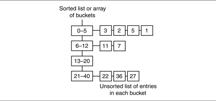
Figure 4.16: Bucketed priority queues
To find the node with the lowest score, you go to the first non-empty bucket and search its contents for the best node.
By changing the number of buckets, you can get just the right blend of adding and removal time. Tweaking the parameters is time consuming, however, and is rarely needed. For very large graphs, such as those representing levels in massively multi-player online games, the speed up can be worth the programming effort. In most cases it is not.
There are still more complex implementations, such as “multi-level buckets,” which have sorted lists of buckets containing lists of buckets containing unsorted items (and so on). I have built a pathfinding system that used a multi-level bucket list, but it was more an act of hubris than a programming necessity, and I wouldn’t do it again!
Implementations
In my experience there is little performance difference between priority heaps and bucketed queues in game pathfinding. I have built production implementations using both approaches. For very large pathfinding problems (with millions of nodes in the graph), bucketed priority queues can be written that are kinder to the processor’s memory cache and are therefore much faster. For indoor levels with a few thousand or tens of thousands of nodes, the simplicity of a priority heap (and the fact that an implementation is often provided by the language or runtime) is often more appealing.
Heuristic Function
The heuristic is often talked about as a function, and it can be implemented as a function. Throughout this book, I’ve preferred to show it in pseudo-code as an object. The heuristic object used in the algorithm has a simple interface:

A Heuristic for Any Goal
Because it is inconvenient to produce a different heuristic function for each possible goal in the world, the heuristic is often parameterized by the goal node. In that way a general heuristic implementation can be written that estimates the distance between any two nodes in the graph. The interface might look something like:

which can then be used to call the pathfinder in code such as:
![]()
Heuristic Speed
The heuristic is called at the lowest point in the loop. Because it is making an estimate, it might involve some algorithmic process. If the process is complex, the time spent evaluating heuristics might quickly dominate the pathfinding algorithm.
While some situations may allow you to build a lookup table of heuristic values, in most cases the number of combinations is huge so this isn’t practical.
Unless your implementation is trivial, I recommend that you run a profiler on the pathfinding system and look for ways to optimize the heuristic. I have seen situations where developers tried to squeeze extra speed from the pathfinding algorithm when over 80% of the execution time was spent evaluating heuristics.
The design of the A* algorithm we’ve looked at so far is the most general. It can work with any kind of cost value, with any kind of data type for nodes, and with graphs that have a huge range of sizes.
This generality comes at a price. There are better implementations of A* for most game pathfinding tasks. In particular, if we can assume that there is only a relatively small number of nodes in the graph (up to 100,000, say, to fit in around 2Mb of memory), and that these nodes can be numbered using sequential integers, then we can speed up our implementation significantly.
I call this node array A* (although you should be aware that I’ve made this name up; strictly, the algorithm is still just A*), and it is described in detail below.
Depending on the structure of the cost values returned and the assumptions that can be made about the graph, even more efficient implementations can be created. Most of these are outside the scope of this book (there are easily a book’s worth of minor variations on A* pathfinding variations), but the most important are given in a brief introduction at the end of this chapter.
The general A* implementation is still useful, however. In some cases you may need a variable number of nodes (if your game’s level is being paged into memory in sections, for example), or there just isn’t enough memory available for more complex implementations. The general A* implementation is still the most common, and can be the absolute fastest on occasions where more efficient implementations are not suitable.
Once again, the biggest factor in determining the performance of A* is the performance of its key data structures: the pathfinding list, the graph, and the heuristic.
Once again, ignoring these, we can look simply at the algorithm (this is equivalent to assuming that all data structure operations take constant time).
The number of iterations that A* performs is given by the number of nodes whose total estimated-path-cost is less than that of the goal. We’ll call this number l, different from n in the performance analysis of Dijkstra. In general, l should be less than n. The inner loop of A* has the same complexity as Dijkstra, so the total speed of the algorithm is O(lm), where m is the average number of outgoing connections from each node, as before. Similarly for memory usage, A* ends with O(lm) entries in its open list, which is the peak memory usage for the algorithm.
In addition to Dijkstra’s performance concerns of the pathfinding list and the graph, we add the heuristic function. In the pseudo-code above, the heuristic value is calculated once per node and then reused. Still, this occurs very low in the loop, in the order of O(l) times. If the heuristic value were not reused, it would be called O(lm) times.
Often, the heuristic function requires some processing and can dominate the execution load of the algorithm. It is rare, however, for its implementation to directly depend on the size of the pathfinding problem. Although it may be time-consuming, the heuristic will most commonly have O(1) execution time and require O(1) memory and so will not have an effect on the order of the performance of the algorithm. This is an example of when the algorithm’s order doesn’t necessarily tell you very much about the real performance of the code.
Node array A* is my name for a common implementation of the A* algorithm that is faster in many cases than the general A* implementation above. In the code we looked at so far, data are held for each node in the open or closed lists, and these data are held as a NodeRecord instance. Records are created when a node is first considered and then moved between the open and closed lists, as required.
There is a key step in the algorithm where the lists are searched for a node record corresponding to a particular node.
Keeping a Node Array
We can make a trade-off by increasing memory use to improve execution speed. To do this, we create an array of all the node records for every node in the whole graph before the algorithm begins. This node array will include records for nodes that will never be considered (hence the waste of memory), as well as for those that would have been created anyway.
If nodes are numbered using sequential integers, we don’t need to search for a node in the two lists at all. We can simply use the node number to look up its record in the array (this is the logic of using node integers that I mentioned at the start of the chapter).
Checking if a Node Is in Open or Closed
We need to find the node data in order to check if we’ve found a better route to a node or if we need to add the node to one of the two lists.
Our original algorithm checked through each list, open and closed, to see if the node was already there. This is a very slow process, especially if there are many nodes in each list. It would be useful if we could look at a node and immediately discover what list, if any, it was contained in.
To find out which list a node is in, we add a new value to the node record. This value tells us which of the three categories the node is in: unvisited, open, or closed. This makes the search step very fast indeed (in fact, there is no search, and we can go straight to the information we need).
The new NodeRecord structure looks like the following:

where the category member is OPEN, CLOSED, or UNVISITED.
The Closed List Is Irrelevant
Because we’ve created all the nodes in advance, and they are located in an array, we no longer need to keep a closed list at all. The only time the closed list is used is to check if a node is contained within it and, if so, to retrieve the node record. Because we have the node records immediately available, we can find the record. With the record, we can look at the category value and see if it has been closed.
The Open List Implementation
We can’t get rid of the open list in the same way because we still need to be able to retrieve the element with the lowest score. We can use the array for times when we need to retrieve a node record, from either open or closed lists, but we’ll need a separate data structure to hold the priority queue of nodes.
Because we no longer need to hold a complete node record in the priority queue, it can be simplified. Often, the priority queue simply needs to contain the node numbers, whose records can be immediately looked up from the node array.
Alternatively, the priority queue can be intertwined with the node array records by making the node records part of a linked list:

Although the array will not change order, each element of the array has a link to the next record in a linked list. The sequence of nodes in this linked list jumps around the array and can be used as a priority queue to retrieve the best node on the open list.
Although I’ve seen implementations that add other elements to the record to support more complex priority queues, my experience is that this general approach leads to wasted memory (most nodes aren’t in the list, after all), unnecessary code complexity (the code to maintain the priority queue can look very ugly), and cache problems (jumping around memory should be avoided when possible). It is preferable to use a separate priority queue of node indices and estimated-total-cost values.
A Variation for Large Graphs
Creating all the nodes in advance is a waste of space if you aren’t going to consider most of them. For small graphs on a PC, the memory waste is often worth it for the speed up. For large graphs, or for consoles with limited memory, it can be problematic.
In C, or other languages with pointers, we can blend the two approaches to create an array of pointers to node records, rather than an array of records themselves, setting all the pointers to NULL initially.
In the A* algorithm, we create the nodes when they are needed, as before, and set the appropriate pointer in the array. When we come to find what list a node is in, we can see if it has been created by checking if its pointer is NULL (if it is, then it hasn’t been created and, by deduction, must be unvisited), if it is there, and if it is in either the closed or open list.
This approach requires less memory than allocating all the nodes in advance, but may still take up too much memory for very large graphs.
On the other hand, for languages with costly garbage collection (such as C#, used in the Unity engine), it can be preferable to allocate objects upfront when the level is loaded, rather than creating them and garbage collecting them at each pathfinding call. This approach is unsuitable in that situation.
The more accurate the heuristic, the less fill A* will experience, and the faster it will run. If you can get a perfect heuristic (one that always returns the exact minimum path distance between two nodes), A* will only consider nodes along with the minimum-cost path: the algorithm becomes O(p), where p is the number of steps in the path.
Unfortunately, to work out the exact distance between two nodes, you typically have to find the shortest route between them. This would mean solving the pathfinding problem—which is what we’re trying to do in the first place! In only a few cases will a practical heuristic be accurate.
For non-perfect heuristics, A* behaves slightly differently depending on whether the heuristic is too low or too high.
Underestimating Heuristics
If the heuristic is too low, so that it underestimates the actual path length, A* takes longer to run. The estimated-total-cost will be biased toward the cost-so-far (because the heuristic value is smaller than reality). So A* will prefer to examine nodes closer to the start node, rather than those closer to the goal. This will increase the time it takes to find the route through to the goal.
If the heuristic underestimates in all possible cases, then the result that A* produces will be the best path possible. It will be the exact same path that the Dijkstra algorithm would generate. This avoids the problem I described earlier with sub-optimal paths.
If the heuristic ever overestimates, however, this guarantee is lost.
In applications where accuracy is more important than performance, it is important to ensure that the heuristic is underestimating. When you read articles about path planning in commercial and academic problems, accuracy is often very important, and so underestimating heuristics abound. This bias in the literature to underestimating heuristics often influences game developers. In practice, try to resist dismissing overestimating heuristics outright. A game isn’t about optimum accuracy; it’s about believability.
Overestimating Heuristics
If the heuristic is too high, so that it overestimates the actual path length, A* may not return the best path. A* will tend to generate a path with fewer nodes in it, even if the connections between nodes are more costly.
The estimated-total-cost value will be biased toward the heuristic. The A* algorithm will pay proportionally less attention to the cost-so-far and will tend to favor nodes that have less distance to go. This will move the focus of the search toward the goal faster, but with the prospect of missing the best routes to get there.
This means that the total length of the path may be greater than that of the best path. Fortunately, it doesn’t mean you’ll suddenly get very poor paths. It can be shown that if the heuristic overestimates by at most x (i.e., x is the greatest overestimate for any node in the graph), then the final path will be no more than x too long.
An overestimating heuristic is sometimes called an “inadmissible heuristic.” This doesn’t mean you can’t use it; it refers to the fact that the A* algorithm no longer returns the shortest path.
Overestimates can make A* faster if they are almost perfect, because they home in on the goal more quickly. If they are only slightly overestimating, they will tend to produce paths that are often identical to the best path, so the quality of results is not a major issue.
But the margin for error is small. As a heuristic overestimates more, it rapidly makes A* perform worse. Unless your heuristic is consistently close to perfect, it can be more efficient to underestimate, and you get the added advantage of getting the correct answer.
Let’s look at some common heuristics used in games.

Figure 4.17: Euclidean distance heuristic
Euclidean Distance
Imagine that the cost values in our pathfinding problem refer to distances in the game level. The connection cost is generated by the distance between the representative points of two regions. This is a common case, especially in first-person shooter (FPS) games where each route through the level is equally possible for each character.
In this case (and in others that are variations on the pure distance approach), a common heuristic is Euclidean distance. It is guaranteed to be underestimating.
Euclidean distance is “as the crow flies” distance. It is measured directly between two points in space, through walls and obstructions.
Figure 4.17 shows Euclidean distances measured in an indoor level. The cost of a connection between two nodes is given by the distance between the representative points of each region. The estimate is given by the distance to the representative point of the goal node, even if there is no direct connection.
Euclidean distance is always either accurate or an underestimate. Traveling around walls or obstructions can only add extra distance. If there are no such obstructions, then the heuristic is accurate. Otherwise, it is an underestimate.

Figure 4.18: Euclidean distance fill characteristics
In outdoor settings, with few constraints on movement, Euclidean distance can be very accurate and provide fast pathfinding. In indoor environments, such as that shown in Figure 4.17, it can be a dramatic underestimate, causing less than optimal pathfinding.
Figure 4.18 shows the fill visualized for a pathfinding task through both tile-based indoor and outdoor levels. With the Euclidean distance heuristic, the fill for the indoor level is dramatic, and performance is poor. The outdoor level has minimal fill, and performance is good.
Cluster Heuristic
The cluster heuristic works by grouping nodes together in clusters. The nodes in a cluster represent some region of the level that is highly interconnected. Clustering can be done automatically using graph clustering algorithms that are beyond the scope of this book. Often, clustering is manual, however, or a by-product of the level design (portal-based game engines lend themselves well to having clusters for each room).
A lookup table is then prepared that gives the smallest path length between each pair of clusters. This is an offline processing step that requires running a lot of pathfinding trials between all pairs of clusters and accumulating their results. A sufficiently small set of clusters is selected so that this can be done in a reasonable time frame and stored in a reasonable amount of memory.
When the heuristic is called in the game, if the start and goal nodes are in the same cluster, then Euclidean distance (or some other fallback) is used to provide a result. Otherwise, the estimate is looked up in the table. This is shown in Figure 4.19 for a graph where each connection has the same cost in both directions.
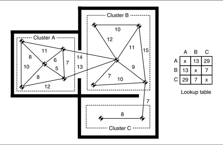
Figure 4.19: The cluster heuristic
The cluster heuristic often dramatically improves pathfinding performance in indoor areas over Euclidean distance, because it takes into account the convoluted routes that link seemingly nearby locations (the distance through a wall may be tiny, but the route to get between the rooms may involve lots of corridors and intermediate areas).
It has one caveat, however. Because all nodes in a cluster are given the same heuristic value, the A* algorithm cannot easily find the best route through a cluster. Visualized in terms of fill, a cluster will tend to be almost completely filled before the algorithm moves on to the next cluster.
If cluster sizes are small, then this is not a problem, and the accuracy of the heuristic can be excellent. On the other hand, the lookup table will be large (and the pre-processing time will be huge).
If cluster sizes are too large, then there will be marginal performance gain, and a simpler heuristic would be a better choice.
I’ve seen and experimented with various modifications to the cluster heuristic to provide better estimates within a cluster, including some that include several Euclidean distance calculations for each estimate. There are opportunities for performance gain here, but as yet there are no accepted techniques for reliable improvement. It seems to be a case of experimenting in the context of your game’s particular level design.

Figure 4.20: Fill patterns indoors
Clustering is intimately related to hierarchical pathfinding, explained in Section 4.6, which also clusters sets of locations together. Some of the calculations we’ll meet there for distance between clusters can be adapted to calculate the heuristics between clusters.
Even without such optimizations, the cluster heuristic is worth trying for labyrinthine indoor levels.
Fill Patterns in A*
Figure 4.20 shows the fill patterns of a tile-based indoor level using A* with different heuristics.
The first example uses a cluster heuristic tailored specifically to this level. The second example used a Euclidean distance, and the final example has a zero heuristic which always returns 0 (the most dramatic underestimate possible). The fill increases in each example; the cluster heuristic has very little fill, whereas the zero heuristic fills most of the level.
This is a good example of the knowledge vs. search trade-off we looked at in Chapter 2.
If the heuristic is more complex and more tailored to the specifics of the game level, then the A* algorithm needs to search less. It provides a good deal of knowledge about the problem. The ultimate extension of this is a heuristic with ultimate knowledge: completely accurate estimates. As we have seen, this would produce optimum A* performance with no search.
On the other hand, the Euclidean distance provides a little knowledge. It knows that the cost of moving between two points depends on their distance apart. This little bit of knowledge helps, but still requires more searching than a better heuristic.

Figure 4.21: Fill patterns outdoors
The zero heuristic has no knowledge, and it requires lots of search.
In our indoor example, where there are large obstructions, the Euclidean distance is not the best indicator of the actual distance. In outdoor maps, it is far more accurate. Figure 4.21 shows the zero and Euclidean heuristics applied to an outdoor map, where there are fewer obstructions. Now the Euclidean heuristic is more accurate, and the fill is correspondingly lower.
In this case Euclidean distance is a very good heuristic, and we have no need to try to produce a better one. In fact, cluster heuristics don’t tend to improve performance (and can dramatically reduce it) in open outdoor levels.
Quality of Heuristics
Producing a heuristic is far more of an art than a science. Its significance is underestimated by AI developers. With the speed of current generation games hardware, many developers use a simple Euclidean distance heuristic in all cases. Unless pathfinding is a significant part of your game’s processor budget, it may not be worth giving it any more thought.
If you do attempt to optimize the heuristic, the only surefire way is to visualize the fill of your algorithm. This can be in-game or using output statistics that you can later examine. Acting blind is dangerous. I’ve found to my cost that tweaks to the heuristic I thought would be beneficial have produced inferior results.
Dijkstra Is A*
It is worth noticing that the Dijkstra algorithm is a subset of the A* algorithm. In A* we calculate the estimated-total-cost of a node by adding the heuristic value to the cost-so-far. A* then chooses a node to process based on this value.
If the heuristic always returns 0, then the estimated-total-cost will always be equal to the cost-so-far. When A* chooses the node with the smallest estimated-total-cost, it is choosing the node with the smallest cost-so-far. This is identical to Dijkstra. A* with a zero heuristic is the point to point version of Dijkstra.
So far I’ve assumed that pathfinding takes place on a graph made up of nodes and connections with costs. This is the world that the pathfinding algorithm knows about, but game environments aren’t made up of nodes and connections.
To squeeze your game level into the pathfinder you need to do some translation—from the geometry of the map and the movement capabilities of your characters to the nodes and connections of the graph and the cost function that values them.
For each pathfinding world representation, we must divide the game level into linked regions that correspond to nodes and connections. The different ways this can be achieved are called division schemes. Each division scheme has three important properties we’ll consider in turn: quantization/localization, generation, and validity.
You might also be interested in Chapter 12, Tools and Content Creation, which looks at how the pathfinding data are created by the level designer or by an automatic process. In a complete game, the choice of world representation will have as much to do with your toolchain as technical implementation issues.
Quantization and Localization
Because the pathfinding graph will be simpler than the actual game level, some mechanism is needed to convert locations in the game into nodes in the graph. When a character decides it wants to reach a switch, for example, it needs to be able to convert its own position and the position of the switch into graph nodes. This process is called quantization.
Similarly, if a character is moving along a path generated by the pathfinder, it needs to convert nodes in the plan back into game world locations so that it can move correctly. This is called localization.

Figure 4.22: Two poor quantizations show that a path may not be viable
Generation
There are many ways of dividing up a continuous space into regions and connections for pathfinding. There are a handful of standard methods used regularly. Each works either manually (the division being done by hand) or algorithmically.
Ideally, of course, we’d like to use techniques that can be run automatically. On the other hand, manual techniques often give the best results, as they can be tuned for each particular game level.
The most common division scheme used for manual techniques is the Dirichlet domain. The most common algorithmic methods are tile graphs, points of visibility, and navigation meshes. Of these, navigation meshes and points of visibility are often augmented so that they automatically generate graphs with some user supervision.
Validity
If a plan tells a character to move along a connection from node A to node B, then the character should be able to carry out that movement. This means that wherever the character is in node A, it should be able to get to any point in node B. If the quantization regions around A and B don’t allow this, then the pathfinder may have created a useless plan.
A division scheme is valid if all points in two connected regions can be reached from each other. In practice, most division schemes don’t enforce validity. There can be different levels of validity, as Figure 4.22 demonstrates.
In the first part of the figure, the issue isn’t too bad. An “avoid walls” algorithm (see Chapter 3) would easily cope with the problem. In the second figure with the same algorithm, it is terminal. Using a division scheme that gave the second graph would not be sensible. Using the first scheme will cause fewer problems. Unfortunately, the dividing line is difficult to predict, and an easily handled invalidity is only a small change away from being pathological.
It is important to understand the validity properties of graphs created by each division scheme; at the very least it has a major impact on the types of character movement algorithm that can be used.
So, let’s look at the major division schemes used in games.
Tile-based levels, in the form of two-dimensional (2D) isometric graphics, were ubiquitous at one point, and now are mostly seen in indie games. The tile is far from dead, however. Although strictly not made up of tiles, a large number of games use grids in which they place their three-dimensional (3D) models. Underlying the graphics is still a regular grid. A game such as Fortnite: Battle Royale [111], for example, places its buildings and structures on a strict grid to allow players’ buildings to connect with them seamlessly.
Such a grid can be simply turned into a tile-based graph. Most real-time strategy (RTS) games still use tile-based graphs extensively, and many outdoor games use graphs based on height and terrain data.
Tile-based levels split the whole world into regular, usually square, regions (although hexagonal regions are occasionally seen in turn-based war simulation games).
Division Scheme
Nodes in the pathfinder’s graph represent tiles in the game world. Each tile in the game world normally has an obvious set of neighbors (the eight surrounding tiles in a rectangular grid, for example, or the six in a hexagonal grid). The connections between nodes correspond to a link between a tile and its immediate neighbors.
Quantization and Localization
We can determine which tile any point in the world is within, and this is often a fast process. In the case of a square grid, we can simply use a character’s x and z coordinates to determine the square it is contained in. For example:

where floor is a function that returns the highest valued integer less than or equal to its argument, and tileX and tileZ identify the tile within the regular grid of tiles.
Similarly, for localization we can use a representative point in the tile (often the center of the tile) to convert a node back into a game location.
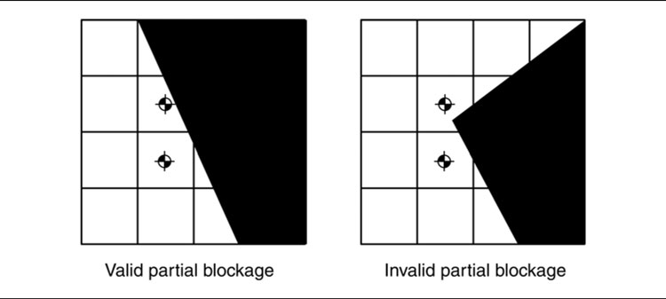
Figure 4.23: Tile-based graph with partially blocked validity
Generation
Tile-based graphs are generated automatically. In fact, because they are so regular (always having the same possible connections and being simple to quantize), they can be generated at runtime. An implementation of a tile-based graph doesn’t need to store the connections for each node in advance. It can generate them as they are requested by the pathfinder.
Most games allow tiles to be blocked. In this case the graph will not return connections to blocked tiles, and the pathfinder will not try to move through them.
For tile-based grids representing outdoor height fields (a rectangular grid of height values), the costs often depend on gradient. The height field data are used to calculate a connection cost based both on distance and on gradient. Each sample in the height field represents the center point of a tile in the graph, and costs can be calculated based on distance and the change in elevation between the two points. In this way it will cost less to go downhill than uphill.
Validity
In many games that use tile-based layouts, a tile will be either completely blocked or completely empty. In this case, if the only tiles that are connected are empty, then the graph will be guaranteed to be valid.
When a graph node is only partially blocked, then the graph may not be valid, depending on the shape of the blockage. Figure 4.23 shows two cases: one in which a partial blockage does not make the graph invalid, and another in which it does.

Figure 4.24: Tile-based plan is blocky
Usefulness
While tile-based levels are one of the easiest to convert to a graph representation, there are often a vast number of tiles in the game. A small RTS level can have many hundreds of thousands of tiles. This means that the pathfinder has to work hard to plan sensible paths.
When the plans returned by the pathfinder are drawn on the graph (using localization for each node in the plan), they can appear blocky and irregular. Characters following the plan will look strange. This is illustrated in Figure 4.24.
While this is a problem with all division schemes, it is most noticeable for tile-based graphs (see Section 4.4.7 on path smoothing for an approach to solving this problem).

Figure 4.25: Dirichlet domains as cones
A Dirichlet domain, also referred to as a Voronoi polygon in two dimensions, is a region around one of a finite set of source points whose interior consists of everywhere that is closer to that source point than any other.
Division Scheme
Pathfinding nodes have an associated point in space called the characteristic point, and the quantization takes place by mapping all locations in the point’s Dirichlet domain to the node. To determine the node for a location in the game, we find the characteristic point that is closest.
The set of characteristic points is usually specified by a level designer as part of the level data.
You can think of Dirichlet domains as being cones originating from the source point. If you view them from the top, as in Figure 4.25, the area of each cone that you see is the area that “belongs” to that source point. This is often a useful visualization for troubleshooting.
The basic idea has been extended to use different falloff functions for each node, so some nodes have a larger “pull” than others in the quantization step. This is sometimes called a weighted Dirichlet domain: each point has an associated weight value that controls the size of its region. Changing the weight is equivalent to changing the slope on the cone; squatter cones end up with larger regions. But care needs to be taken. Once you change the slope, you can get strange effects.
Figure 4.26 shows the Dirichlet domains in a passageway. You can see that the end of the passageway belongs to the wrong source point: the fat cone has peaked back out. This can make it difficult to debug pathfinding problems.

Figure 4.26: Problem domains with variable falloff
If you are manually assigning weighted Dirichlet domains, it’s a good idea to have them displayed to check for overlapping problems.
Connections are placed between bordering domains. The pattern of connections can be found using a mathematical structure that has deep connections to Voronoi diagrams, called a Delaunay triangulation. The edges of the Delaunay triangulation are the connections in the graph, and the vertices are the characteristic points of the domains. Creating a Delaunay triangulation of a set of points is beyond the scope of this book. There are many websites dedicated to the algorithms for constructing a Delaunay triangulation. For an academic survey of the approaches, see [66].
Many developers don’t bother with a mathematically correct algorithm, however. They either make the artist specify connections as part of their level design, or they ray cast between points to check for connections (see the points of visibility method below). Even if you use the Delaunay triangulation method, you will need to check that domains that touch can actually be moved between, as there might be a wall in the way, for example.
Quantization and Localization
Positions are quantized by finding the characteristic point that is closest.
Searching through all points to find the closest is a time-consuming process (an O(n) process, where n is the number of domains). Typically, we will use some kind of spatial partitioning algorithm (quad-tree, octree, binary space partition, or multi-resolution map) to allow us to consider only those points that are nearby.
The localization of a node is given by the position of the characteristic point that forms the domain (i.e., the tip of the cone in the example above).
Validity
Dirichlet domains can form intricate shapes. There is no way to guarantee that traveling from a point in one domain to a point in a connected domain will not pass through a third domain. This third domain might be impassable and might have been discounted by the pathfinder. In this case, following the path will lead to a problem. Strictly, therefore, Dirichlet domains produce invalid graphs.
In practice, however, the placement of nodes is often based on the structure of obstacles. Obstacles are not normally given their own domains, and so the invalidity of the graph is rarely exposed.
To make sure, you can provide some kind of backup mechanism (like an avoid walls steering behavior) to solve the issue and avoid your characters happily running headfirst into walls.
Usefulness
Dirichlet domains are very widely used. They have the advantage of being very easy to program (automatic generation of connections aside) and easy to change. It is possible to rapidly change the structure of the pathfinding graph in a level-editing tool without having to change any level geometry.
It can be shown that the optimal path through any 2D environment will always have inflection points (i.e., points on the path where the direction changes) at convex vertices in the environment. If the character that is moving has some radius, these inflection points are replaced by arcs of a circle at a distance away from the vertex. This is illustrated in Figure 4.27.
In three dimensions, the same thing applies, but inflection points are located at either convex polygon edges or vertices.
In either case, we can approximate these inflection points by choosing a characteristic point that is shifted out from the vertices a short distance. This will not give us the curves, but it will give us believable paths. These new characteristic points can be calculated from the geometry by extending out the geometry a little way and calculating where the edges of the new geometry are.
Division Scheme
Since these inflection points naturally occur in the shortest path, we can use them as nodes in the pathfinding graph.
Working on the actual level geometry will provide us with far too many inflection points. A simplified version is needed so that we can find inflection points where the large-scale geometry changes. It may be possible to take these points from collision geometry, or they may need to be generated specially.

Figure 4.27: Path with inflections at vertices

Figure 4.28: Points of visibility graph bloat
These inflection points can then be used as the node locations to build a graph.
To work out how these points are connected, rays are cast between them, and a connection is made if the ray doesn’t collide with any other geometry. This is almost equivalent to saying that one point can be seen from the other. For this reason it is called a “points of visibility” approach. In many cases the resultant graph is huge. A complex cavern, for example, may have many hundreds of inflection points, each of which may be able to see most of the others. This is shown in Figure 4.28.
Quantization, Localization, and Validity
Points of visibility are usually taken to represent the centers of Dirichlet domains for the purpose of quantization.
In addition, if Dirichlet domains are used for quantization, points quantized to two connected nodes may not be able to reach each other. As we saw in Dirichlet domains above, this means that the graph is strictly invalid.
Usefulness
Despite its major shortcomings, a points of visibility approach is a relatively popular method for automatic graph generation.
However, in my opinion the results are not worth the effort. Initial results are positive but a lot of fiddling and clearing up by hand is needed to produce a final graph, which defeats the object. I’d recommend looking at navigation meshes instead: they share a lot of the same benefits, but dramatically reduce the number of connections, and require much less adjustment.
Tile-based graphs, Dirichlet domains, and points of visibility are all useful division schemes to have in your toolbox, but the majority of modern games with 3D environments use navigation meshes (often abbreviated to “navmesh”) for pathfinding.
The navigation mesh approach to pathfinding takes advantage of the fact that the level designer already needs to specify the way the level is connected, the regions it has, and whether there is any AI in the game or not. The level itself is made up of polygons connected to other polygons. We can use this graphical structure as the basis of a pathfinding representation.
Division Scheme
Many games use floor polygons, as defined by artists, as regions. Each polygon acts as a node in the graph, as shown in Figure 4.29.
The graph is based on the mesh geometry of the level and therefore is often called a navigation mesh, or just “navmesh.”
As the number of polygons in a scene has increased dramatically, over the last 15 years, it has become rarer for floors to be represented by a small number of large triangles. In the same way that the points-of-visibility approach requires simplified stand-in geometry to make its graphs tractable, navigation meshes are rarely able to work on the same geometry as the renderer. It is fairly common, however, for a scene to require a separate simplified collision geometry. This geometry is usually simple enough to build a navigation mesh.
Regardless of the source of the geometry, nodes in the graph represent polygons. Two nodes are connected if their corresponding polygons share an edge. Floor polygons are typically triangles, but may be quads. Nodes therefore have either three or four connections.

Figure 4.29: Polygonal mesh graph
Creating a navigation mesh usually involves the artist labeling particular polygons as floor in their modeling package. They may need to do this anyway to specify sound effects or grip characteristics. Navigation meshes require less artist intervention than other approaches, with the exception of tile-based graphs.
Quantization and Localization
A position is localized into the floor polygon that contains it. We could search a large number of polygons to find the right one, or use a complex spatial data structure to speed up the query. But often we are better off using a coherence assumption.
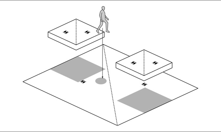
Figure 4.30: Quantization into a gap
Coherence refers to the fact that, if we know which location a character was in at the previous frame, it is likely to be in the same node or an immediate neighbor on the next frame. We can check these nodes first. This approach is useful in lots of division schemes, but is particularly crucial when dealing with navigation maps.
However we determine the node, care must be taken when a character is not touching the floor. If we simply find the polygon vertically below it and quantize it there, it is possible for the character to be placed in a completely inappropriate node as it falls or jumps. In Figure 4.30, for example, the character is quantized to the bottom of the room, even though it is actually using the walkways above. This may then cause the character to replan its route as if it were in the bottom of the room; not the desired effect. Coherence can help here too, avoiding assigning a character to a node far from where it was last seen. But coherence alone does not solve all problems. Some special case code is generally needed that knows when a character is jumping, and either postpones pathfinding, or uses trajectory prediction to determine where it will land.
Localization can choose any point in the polygon, but normally uses the geometric center (the average position of its vertices). This works fine for triangles. For quads or polygons with more sides, the polygon must be convex for this to work. Geometric primitives used in graphics or physics engines have this requirement anyway. So if we are using the same primitives used for rendering or collision detection, we are safe.

Figure 4.31: Non-interpolation of the navigation mesh
Validity
The regions generated by navigation meshes can be problematic. We have assumed that any point in one region can move directly to any point in a connected region, but this may not be the case. See Figure 4.31 for an example that contains a pair of triangles with areas where traveling directly between them causes a collision.
Because floor polygons are created by the level designer, this situation can be mitigated. The geometry naturally created by most sensible level designers does not suffer from major problems.
Usefulness
Using this approach also requires additional processing to take into account the agent’s geometry. Since not all locations in a floor polygon may be occupied by a character (some are too close to walls or other obstacles), some trimming is required; this may affect the connections generated by finding shared edges. This problem is especially evident at convex areas such as doorways.
For the occasional game that needs it, this approach offers the additional benefit of allowing characters to plan routes up walls, across ceilings, or for any other kind of geometry. This might be useful if characters stick to walls, for example. It is much more difficult to achieve the same result with other world representations.

Figure 4.32: Portal representation of a navigation mesh
Edges as Nodes
Floor polygons can also be converted into a pathfinding graph by assigning nodes to the edges between polygons and using connections across the face of each polygon. Figure 4.32 illustrates this.
This approach is also commonly used in association with portal-based rendering, where nodes are assigned to portals and where connections link all portals within the line of sight of one another. Portal rendering is a graphics technique where the geometry of the whole level is split into chunks, linked by portals, a 2D polygonal interface between the regions. By separating the level into chunks, it is easier to test which chunks need to be drawn, reducing the rendering time. Full details are beyond the scope of this book, but should be covered in any good modern text on game engine design.
In the navigation mesh, the edges of every floor polygon act like a portal and therefore have their own node. We don’t need to do the line-of-sight tests. By definition, each edge of a convex floor polygon can be seen from every other edge.
Some articles suggest that the nodes on the edges of floor polygons are placed dynamically in the best position as the pathfinder does its work. Depending on the direction that the character is moving, the nodes should be at a different location. This is shown in Figure 4.33.
This is a kind of continuous pathfinding, and we’ll look at the algorithm for continuous pathfinding later in the chapter. In my opinion, however, this approach is overkill. It is better to work with the faster fixed graph. If the resulting path looks too crinkled, then a path smoothing step (which I’ll cover in Section 4.4.7) is perfectly sufficient.
Both the polygon-as-node and the edge-as-node representations are known as navigation meshes. Often, one or the other approach is assumed, so it is worth making sure that whatever source you are using makes it clear which version they are talking about.

Figure 4.33: Different node positions for different directions
4.4.5 NON-TRANSLATIONAL PROBLEMS
There is nothing in the above discussion about regions and connections that requires us to be dealing with positions only.
In some tile-based games, where agents cannot turn quickly, tiles are created for each location and orientation, so an agent with a large turning circle can only move to a tile with a slightly different orientation in one step.
In Figure 4.34 an agent cannot turn without moving and can only turn by 90° at a time. Nodes A1, A2, A3, and A4 all correspond to the same location. They represent different orientations, however, and they have different sets of connections. The quantization of an agent’s state into a graph node needs to take account of both its position and its orientation.
The result from planning on this graph will represent a sequence of translations and rotations. A plan on the graph in Figure 4.34 is shown in Figure 4.35.
In the simplest cases, where we are interested in finding the shortest path, the cost of a connection can represent distance. The higher the cost, the larger the distance between nodes.
If we are interested in finding the quickest path to move along, we could use costs that depend on time. This isn’t the same thing as distance; it is quicker to run 10 feet than to climb a 10-foot ladder.
Navigation software that plans a route on the road network uses exactly the algorithms in this chapter. Navigation apps often give users a choice between the fastest route and the shortest route, by modifying the cost function in this way.

Figure 4.34: A non-translational tile-based world
In games, we can add all sorts of other concerns to the costs on a graph. In an RTS, for example, we could make certain connections more costly if they were exposed to enemy fire or if they wandered too near to dangerous terrain. The final path would then be the one with the lowest danger.
Often, the cost function is a blend of many different concerns, and there can be different cost functions for different characters in a game. A reconnaissance squad, for example, may be interested in visibility and speed. A heavy artillery weapon would be more interested in terrain difficulty. Pathfinding that incorporates these concerns is called tactical pathfinding, and we’ll look at it in depth in Chapter 6.
A path that travels from node to node through a graph can appear erratic. Sensible node placing can give rise to very odd looking paths. Figure 4.36 shows a section of a level with nodes placed in a reasonable manner. The path constantly switches direction; a character following the path will not look intelligent.
Some world representations are more prone to rough paths than others. Portal representations with points of visibility connections can give rise to very smooth paths, while tile-based graphs tend to be highly erratic. The final appearance also depends on how characters act on the path. If they are using some kind of path following steering behavior (see Chapter 3), then the path will be gently smoothed by the steering. It is worth testing your game before assuming the path will need additional modification.

Figure 4.35: Plan on a non-translational tile graph
For some games, path smoothing is essential to get the AI looking smart. The path smoothing algorithm is relatively simple to implement but involves queries to the level geometry. Therefore, it can be somewhat time-consuming.
The Algorithm
We start with an input path, as generated from A*, or another pathfinding algorithm. We will assume in this algorithm that there is a clear route between any two adjacent nodes in the input path. In other words, we are assuming that the division scheme is valid.
To smooth the input path, we first create a new empty path. This is the output path. We add the start node to it. The output path will start and end at the same nodes as the input path.

Figure 4.36: Smoothed path with optimal smoothing indicated
Starting at the third node in the input path, a ray is cast to each node in turn from the last node in the output path. We start at the third node because we are assuming that there is a clear line (a passed ray cast) between the first and second nodes.
When a ray fails to get through, the previous node in the input path is added to the output path. Ray casting starts again from the next node in the input path. When the end node is reached, it is added to the output path. The output path is used as the path to follow.
Figure 4.36 illustrates a path that has been smoothed with this algorithm.
Although this algorithm produces a smooth path, it doesn’t search all possible smoothed paths to find the best one. The figure shows the smoothest possible path in our example; it cannot be generated by this algorithm. To generate the smoothest path, we’d need another search among all possible smoothed paths. This is rarely, if ever, necessary.
Pseudo-Code
The path smoothing algorithm takes an input path made up of nodes and returns a smoothed output path:
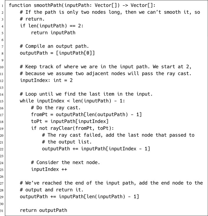
Data Structures and Interfaces
The pseudo-code works with paths that are a list of nodes. The pathfinding algorithms so far have returned a path as a list of connections. Although we could take this kind of path as input, the output path cannot be made up of connections. The smoothing algorithm links nodes that are in line of sight, but are unlikely to have any connections between them (if they were connected in the graph, the pathfinder would have found the smoothed route directly, unless their connections had dramatically large costs).
Performance
The path smoothing algorithm is O(1) in memory, requiring only temporary storage. It is O(n) in time, where n is the number of nodes in the path.
The majority of the time spent in this algorithm is spent carrying out ray casting checks.
With a good heuristic, A* is a very efficient algorithm. Even simple implementations can plan across many tens of thousands of nodes in a frame. Even better performance can be achieved using additional optimizations, such as those we considered in the previous sections.
Many game environments are huge and contain hundreds of thousands or even millions of locations. Massively multi-player online games (MMOGs) may be hundreds of times larger still. While it is possible to run an A* algorithm on an environment of this size, it will be extremely slow and take a huge amount of memory. The results are also less than practical. If a character is trying to move between cities in an MMOG, then a route that tells it how to avoid a small boulder in the road five miles away is overkill. This problem can be better solved using hierarchical pathfinding.
Often, many different plans need to be made in quick succession: a whole army may need to plan its routes through a battlefield, for example. Other techniques, such as dynamic pathfinding, can increase the speed of replanning, and a number of A* variations dramatically reduce the amount of memory required to find a path, at the cost of some performance.
The remainder of this chapter will look at some of these issues in detail and will try to give a flavor for the range of different A* variations that are possible.
Hierarchical pathfinding plans a route in much the same way as a person would. We plan a course overview route first and then refine it as needed. The high-level overview route might be “To get to the rear parking lot, we’ll go down the stairs, out of the front lobby, and around the side of the building,” or “We’ll go through the office, out the fire door, and down the fire escape.” For a longer route, the high-level plan would be even more abstract: “To get to the London office, we’ll go to the airport, catch a flight, and get a cab when we land.”
Each stage of the path will consist of another route plan. To get to the airport, for example, we need to know the route. The first stage of this route might be to get to the car. This, in turn, might require a plan to get to the rear parking lot, which in turn will require a plan to maneuver around the desks and get out of the office.
This is a very efficient way of pathfinding. To start with, we plan the abstract route, take the first step of that plan, find a route to complete it, and so on down to the level where we can actually move. After the initial multi-level planning, we only need to plan the next part of the route when we complete a previous section. When we arrive at the bottom of the stairs, on our way to the parking lot (and from there to the London office), we plan our route through the lobby. When we arrive at our car, we then have completed the “get to the car” stage of our more abstract plan, and we can plan the “drive to the airport” stage.
The plan at each level is typically simple, and we split the pathfinding problem over a long period of time, only doing the next bit when the current bit is complete.
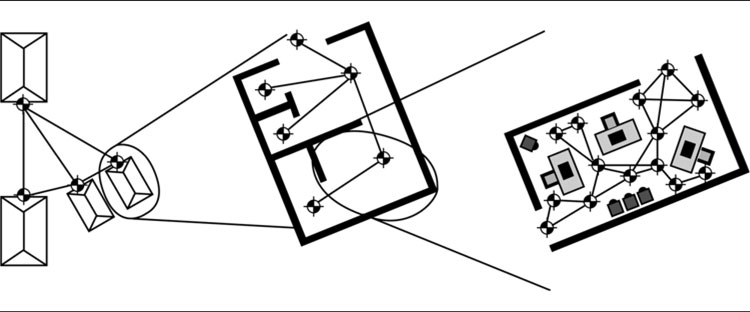
Figure 4.37: Hierarchical nodes
4.6.1 THE HIERARCHICAL PATHFINDING GRAPH
To be able to pathfind at higher levels we can still use the A* algorithm and all its optimizations. In order to support hierarchical pathfinding, we need to alter the graph data structure.
Nodes
This is done by grouping locations together to form clusters. The individual locations for a whole room, for example, can be grouped together. There may be 50 navigation points in the room, but for higher level plans they can be treated as one. This group can be treated as a single node in the pathfinder, as shown in Figure 4.37.
This process can be repeated as many times as needed. The nodes for all the rooms in one building can be combined into a single group, which can then be combined with all the buildings in a complex, and so on. The final product is a hierarchical graph. At each level of the hierarchy, the graph acts just like any other graph you might pathfind on.
To allow pathfinding on this graph, you need to be able to convert a node at the lowest level of the graph (which is derived from the character’s position in the game level) to one at a higher level. This is the equivalent of the quantization step in regular graphs. A typical implementation will store a mapping from nodes at one level to groups at a higher level.
Connections
Pathfinding graphs require connections as well as nodes. The connections between higher level nodes need to reflect the ability to move between grouped areas. If any low-level node in one group is connected to any low-level node in another group, then a character can move between the groups, and the two groups should have a connection.

Figure 4.38: A hierarchical graph
Figure 4.38 shows the connections between two nodes based on the connectivity of their constituent nodes at the next level down in the hierarchy.
Connection Costs
The cost of a connection between two groups should reflect the difficulty of traveling between them. This can be specified manually, or it can be calculated from the cost of the low-level connections between those groups.
This is a complex calculation, however. Figure 4.39 shows that the cost of moving from group C to group D depends on whether you entered group C from group A (a cost of 5) or from group B (a cost of 2).
In general, the grouping should be chosen to minimize this problem, but it cannot be resolved easily.
There are three heuristics that are commonly used, straight or blended, to calculate the connection cost between groups.

Figure 4.39: A tile-based representation of a level with groups marked
Minimum Distance
The first is minimum distance. This heuristic says that the cost of moving between two groups is the cost of the cheapest link between any nodes in those groups. This makes sense because the pathfinder will try to find the shortest route between two locations. In the example above, the cost of moving from C to D would be 1. Note that if you entered C from either A or B, it would take more than one move to get to D. The value of 1 is almost certainly too low, but this may be an important property depending on how accurate you want your final path to be.
Maximin Distance
The second is the “maximin” distance. For each incoming link, the minimum distance to any suitable outgoing link is calculated. This calculation is usually done with a pathfinder. The largest of these values is then added to the cost of the outgoing link and used as the cost between groups.
In the example, to calculate the cost of moving from C to D, two costs are calculated: the minimum cost from C1 to C5 (4) and the minimum cost from C6 to C7 (1). The largest of these (C1 to C5) is then added to the cost of moving from C5 to D1 (1). This leaves a final cost from C to D of 5. To get from C to D from anywhere other than C1, this value will be too high. Just like the previous heuristic, this may be what you need.
Average Minimum Distance
A value in the middle of these extremes is sometimes better. The “average minimum” distance is a good general choice. This can be calculated in the same way as the maximin distance, but the values are averaged, rather than simply selecting the largest. In our example, to get from C to D coming from B (i.e., via C6 and C7), the cost is 2, and when coming from A (via C2 to C5) it is 5. So the average cost of moving from C to D is
Summary of the Heuristics
The minimum distance heuristic is very optimistic. It assumes that there will never be any cost to moving around the nodes within a group. The maximin distance heuristic is pessimistic. It finds one of the largest possible costs and always uses that. The average minimum distance heuristic is pragmatic. It gives the average cost you’ll pay over lots of different pathfinding requests.
The approach you choose isn’t only dictated by accuracy; each heuristic has an effect on the kinds of paths returned by a hierarchical pathfinder. We’ll return to why this is so after we look in detail at the hierarchical pathfinding algorithm.
4.6.2 PATHFINDING ON THE HIERARCHICAL GRAPH
Pathfinding on a hierarchical graph uses the normal A* algorithm. It applies the A* algorithm several times, starting at a high level of the hierarchy and working down. The results at high levels are used to limit the work it needs to do at lower levels.
Algorithm
Because a hierarchical graph may have many different levels, the first task is to find which level to begin on. We want as high a level as possible, so we do the minimum amount of work. However, we also don’t want to be solving trivial problems either.
The initial level should be the first in which the start and goal locations are not at the same node. Any lower and we would be doing unnecessary work; any higher and the solution would be trivial, since the goal and start nodes are identical.
In Figure 4.38 the pathfinding should take place initially at level 2, because level 3 has the start and end locations at the same node.
Once a plan is found at the start level, then the initial stages of the plan need to be refined. We refine the initial stages because those are the most important for moving the character. We won’t initially need to know the fine detail of the end of the plan; we can work that out nearer the time.
The first stage in the high-level plan is considered (occasionally, it can be useful to consider the first few; this is a heuristic that needs to be tried for different game worlds). This small section will be refined by planning at a slightly lower level in the hierarchy.
The start point is the same, but if we kept the end point the same we’d be planning through the whole graph at this level, so our previous planning would be wasted. So, the end point is set at the end of the first move in the high-level plan.
For example, if we are planning through a set of rooms, the first level we consider might give us a plan that takes us from where our character is in the lobby to the guardroom and from there to its goal in the armory. At the next level we are interested in maneuvering around obstacles in the room, so we keep the start location the same (where the character currently is), but set the end location to be the doorway between the lobby and the guardroom. At this level we will ignore anything we may have to do in the guardroom and beyond.
This process of lowering the level and resetting the end location is repeated until we reach the lowest level of the graph. Now we have a plan in detail for what the character needs to do immediately. We can be confident that, even though we have only looked in detail at the first few steps, making those moves will still help us complete our goal in a sensible way.
Pseudo-Code
The algorithm for hierarchical pathfinding has the following form:

Data Structures and Interfaces
In the code above I have made some additions to our graph data structure. Its interface now looks like the following:

The setLevel method switches the graph into a particular level. All calls to getConnections then act as if the graph was just a simple, non-hierarchical graph at that level. The A* function has no way of telling that it is working with a hierarchical graph; it doesn’t need to.
The getNodeAtLevel method converts nodes between different levels of the hierarchy. When increasing the level of a node, we can simply find which higher level node it is mapped to. When decreasing the level of a node, however, one node might map to any number of nodes at the next level down.
This is just the same process as localizing a node into a position for the game. There are any number of positions in the node, but we select one in localization. The same thing needs to happen in the getNodeAtLevel method. We need to select a single node that can be representative of the higher level node. This is usually a node near the center, or it could be the node that covers the greatest area or the most connected node (an indicator that it is a significant one for route planning).
In an implementation I wrote for a previous company I used a fixed node at a lower level, generated by finding the node closest to the center of all those mapped to the same higher level node. This is a fast, geometric, pre-processing step that doesn’t require human intervention. This node was then stored with the higher level node, where it could be returned when needed without additional processing. This worked well and produced no problematic plans, but you may prefer to try different methods or manual specification by the level designer.
Performance
The A* algorithm has the same performance characteristics as before, since we are using it unchanged.
The hierarchical pathfinder function is O(1) in memory and O(p) in time, where p is the number of levels in the graph. Overall, the function is O(plm) in time. Obviously, this appears to be slower than the basic pathfinding algorithm.
And it may be. It is possible to have a hierarchical graph that is so poorly structured that the overall performance is lower. In general, however, there are p stages of the O(lm) A* algorithm, but in each case the number of iterations (l) should be much smaller than a raw A* call, and the practical performance will be significantly higher.
For large graphs (with millions of nodes, for example) it is not uncommon to see two orders of magnitude improvement in running speed, using several levels in the hierarchy. I used this technique in a performance demo in 2003 to allow characters to pathfind on a graph with a hundred million nodes in real time.
4.6.3 HIERARCHICAL PATHFINDING ON EXCLUSIONS
A character can only follow the plan generated by the hierarchical pathfinding algorithm for a short time. When it reaches the end of the lowest level plan, it will need to plan its next section in more detail.
When its plan runs out, the algorithm is called again, and the next section is returned. If you use a pathfinding algorithm that stores plans (see Section 4.7, Other Ideas in Pathfinding), the higher level plans won’t need to be rebuilt from scratch (although that is rarely a costly process).
In some applications, however, you might prefer to get the whole detailed plan up front.
In this case hierarchical pathfinding can still be used to make the planning more efficient.
The same algorithm is followed, but the start and end locations are never moved. Without further modification, this would lead to a massive waste of effort, as we are performing a complete plan at each level.
To avoid this, at each lower level, the only nodes that the pathfinder can consider are those that are within a group node that is part of the higher level plan.
For example, in Figure 4.40 the first high-level plan is shown. When the low-level plan is made (from the same start and end locations), all the shaded nodes are ignored. They are not even considered by the pathfinder. This dramatically reduces the size of the search, but it can also miss the best route, as shown.

Figure 4.40: Switching off nodes as the hierarchy is descended
It is not as efficient as the standard hierarchical pathfinding algorithm, but it can still be a very powerful technique.
4.6.4 STRANGE EFFECTS OF HIERARCHIES ON PATHFINDING
It is important to realize that hierarchical pathfinding gives an approximate solution. Just like any other heuristic, it can perform well in certain circumstances and poorly in others. It may be that high-level pathfinding finds a route that could be shortcut at a lower level. This shortcut will never be found, because the high-level route is “locked in” and can’t be reconsidered.
The source of this approximation is the link costs we calculated when we turned the lowest level graph into a hierarchical graph. Because no single value can accurately represent all the possible routes through a group of nodes, they will always be wrong some of the time.
Figures 4.41 and 4.42 show cases in which each method of calculating the link cost produces the wrong path.
In Figure 4.41 we see that because the minimum cost is 1 for all connections between rooms, the path planner chooses the route with the smallest number of rooms, rather than the much more direct route. The minimum cost method works well for situations where each room costs roughly the same to traverse.
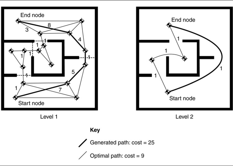
Figure 4.41: Pathological example of the minimum method
We see in Figure 4.42 that the obvious, direct route is not used because the connection has a very large maximin value. The maximin algorithm works better when every route has to pass through many rooms.
In the same example, using the average minimum method does not help, since there is only one route between rooms. The direct route is still not used. The average minimum method often performs better than the maximin method, except in cases where most of the rooms are long and thin with entrances at each end (networks of corridors, for example) or when there are few connections between rooms.
The failure of each of these methods doesn’t indicate that there is another, better method that we haven’t discussed yet; all possible methods will be wrong in some cases. Whatever method you use, it is important to understand what effects the wrongness has. One of the scenarios above, or a blend of them, is likely to provide the optimum trade-off for your game, but finding it is a matter of tweaking and testing.

Figure 4.42: Pathological example of the maximin method
In a single-player game or a level-based multi-player game, all the detail for a level is typically unique. If multiple copies of the same geometry are used, then they are usually tweaked to be slightly different. The pathfinding graph is unique for the whole level, and it doesn’t make sense to use the same subsection of the graph for more than one area in the level.
For massively multi-player games, or large open world RPGs, the whole world can consist of a single level. There is no way to have the same detailed, unique modeling on this scale. Most games at this scale use one large definition for the topology of the landscape (typically, a height field grid that can be represented to the pathfinding system as a tile-based graph). Onto this landscape buildings are placed, either as a whole or as entrances to a separate minilevel representing the inside of the building. Tombs, castles, caves, or spaceships can all be implemented in this way. I’ve used the technique to model bridges connecting islands in a squad-based game, for example. For simplicity, I’ll refer to all these mini-levels as buildings in this section.
These placed buildings are sometimes unique (for special areas with significance to the game content). In most cases, however, they are somewhat generic. There may be 20 farmhouse designs, for example, but there may be hundreds of farmhouses across the world. In the same way that the game wouldn’t store many copies of the geometry for the farmhouse, it shouldn’t store many copies of the pathfinding graph.
We would like to be able to instantiate the pathfinding graph so that it can be reused for every copy of the building.
Algorithm
For each type of building in the game, we have a separate pathfinding graph. The pathfinding graph contains some special connections labeled as “exits” from the building. These connections leave from nodes that we’ll call “exit nodes.” They are not connected to any other node in the building’s graph.
For each instance of a building in the game, we keep a record of its type and which nodes in the main pathfinding graph (i.e., the graph for the whole world) each exit is attached to. Similarly, we store a list of nodes in the main graph that should have connections into each exit node in the building graph. This provides a record of how the building’s pathfinding graph is wired into the rest of the world.
Instance Graph
The building instance presents a graph to be used by the pathfinder. Let’s call this the instance graph. Whenever it is asked for a set of connections from a node, it refers to the corresponding building type graph and returns the results.
To avoid the pathfinder getting confused about which building instance it is in, the instance makes sure that the nodes are changed so that they are unique to each instance.
The instance graph is simply acting as a translator. When asked for connections from a node, it translates the requested node into a node value understood by the building graph. It then delegates the connection request to the building graph, as shown in Figure 4.43. Finally, it translates the results so that the node values are all instance-specific again and returns the result to the pathfinder.
For exit nodes, the process adds an additional stage. The building graph is called in the normal way, and its results are translated. If the node is an exit node, then the instance graph adds the exit connections, with destinations set to the appropriate nodes in the main pathfinding graph.
Because it is difficult to tell the distance between nodes in different buildings, the connection costs of exit connections are often assumed to be zero. This is equivalent to saying that the source and destination nodes of the connection are at the same point in space.
World Graph
To support entrance into the building instance, a similar process needs to occur in the main pathfinding graph. Each node requested has its normal set of connections (the eight adjacent neighbors in a tile-based graph, for example). It may also have connections into a building instance. If so, the world graph adds the appropriate connection to the list. The destination node of this connection is looked up in the instance definition, and its value is in instance graph format. This is illustrated in Figure 4.44.

Figure 4.43: The delegation in progress
The pathfinder, as we’ve implemented it in this chapter, can only handle one graph at a time. The world graph manages all the instance graphs to make it appear as if it is generating the whole graph. When asked for the connections from a node, it first works out which building instance the node value is from or if it is from the main pathfinding graph. If the node is taken from a building, it delegates to that building to process the getConnections request and returns the result unchanged. If the node is not taken from a building instance, it delegates to the main pathfinding graph, but this time adds connections for any entrance nodes into a building.
If you are building a pathfinder from scratch to use in a game where you need instancing, it is possible to include the instancing directly in the pathfinding algorithm, so it makes calls to both the top-level graph and the instanced graphs. This approach makes it much more difficult to later incorporate other optimizations such as hierarchical pathfinding, or node array A*, however, so we’ll stick with the basic pathfinding implementation here.
Pseudo-Code
To implement instanced geometry we need two new implicit graphs: one for building instances and one for the main pathfinding graph.

Figure 4.44: An instance in the world graph
In the code below I have added the data used to store the building instance with the instance graph class, since the same data are needed for each. The instance graph implementation therefore has the following form:

The main pathfinding graph has the following structure:
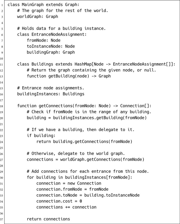
Data Structures and Interfaces
In the instance graph class, we access the exit nodes as a hash, indexed by node number and returning a list of exit node assignments. This process is called every time the graph is asked for connections, so it needs to be implemented in as efficient a manner as possible. The building instances structure in the world graph class is used in exactly the same way, with the same efficiency requirements.
The building instances structure also has a getBuilding method in the pseudo-code above. This method takes a node and returns a building instance from the list if the node is part of the instance graph. If the node is part of the main pathfinding graph, then the method returns a null value. This method is also highly speed critical. Because a range of node values is used by each building, however, it can’t be easily implemented as a hash table. A good solution is to perform a binary search on the nodeOffsets of the buildings. A further speed up can be made using coherence, taking advantage of the fact that if the pathfinder requests a node in a building instance, it is likely to follow it with requests to other nodes in the same building.
Implementation Notes
The translation process between instance node values and building node values assumes that nodes are numeric values. This is the most common implementation of nodes. However, they can be implemented as opaque data instead. In this case the translation operations (adding and subtracting nodeOffset in the pseudo-code) would be replaced by some other operation on the node data type.
The main pathfinding graph for a tile-based world is usually implicit. Rather than delegating from a new implicit graph implementation to another implicit implementation, it is probably better to combine the two. The getConnections method compiles the connections to each neighboring tile, as well as checks for building entrances.
Performance
Both the instance graph and the world graph need to perform a hash lookup for entrance or exit connections. This check takes place at the lowest part of the pathfinding loop and therefore is speed critical. For a well-balanced hash, the speed of hash lookup approaches O(1).
The world graph also needs to look up a building instance from a node value. In the case where nodes are numeric, this cannot be performed using a reasonably sized hash table. A binary search implementation is O(log2 n) in time, where n is the number of buildings in the world. Judicial use of caching can reduce this to almost O(1) in practice, although pathological graph structures can theoretically foil any caching scheme and give the O(log2 n) worst case.
Both algorithms are O(1) in memory, requiring only temporary storage.
Weaknesses
This approach introduces a fair amount of complexity low down in the pathfinding loop. The performance of the pathfinder is extremely sensitive to inefficiencies in the graph data structure. I have seen a halving of execution speed by using this method. It is not worth the extra time if the game level is small enough to create a single master graph.
For massive worlds with instanced buildings, however, a single graph may not be an option, and instanced graphs are the only way to go. I would personally be reluctant to consider using instanced graphs in a production environment unless the pathfinding system was hierarchical (if the graph is big enough to need instanced buildings, it is big enough to need hierarchical pathfinding). This has the added advantage that each building instance can be treated as a single node higher up the hierarchy. When using a hierarchical pathfinding algorithm, moving to instanced geometry usually produces a much smaller drop in pathfinding speed, because instanced graphs are only considered when they are part of the plan.
Setting Node Offsets
In order for this code to work, we need to make sure that every building instance has a unique set of node values. The node values should not only be unique within instances of the same building type, but also between different building types. If node values are numeric, this can be simply accomplished by assigning the first building instance a nodeOffset equal to the number of nodes in the main pathfinding graph. Thereafter, subsequent building instances have offsets which differ from the previous building by the number of nodes in the previous building’s graph.
For example, let’s say we have a pathfinding graph of 10,000 nodes and three building instances. The first and third buildings are instances of a type with 100 nodes in the graph. The second building has 200 nodes in its graph. Then the node offset values for the building instances would be 10,000, 10,200, and 10,300.
4.7 OTHER IDEAS IN PATHFINDING
There are many variations on the A* algorithm that have been developed for specific applications. It would take a book this size to describe them all. This section takes a whirlwind tour of some of the most interesting. There are pointers to more information, including algorithm specifications, in the references at the end of the book.
In many applications there may be more than one possible node in the graph that is a goal. If a character is pathfinding to an alarm point, for example, then any alarm will do, and there will be multiple possible goals.
Rather than checking if a node is the goal, we need to check if the node is a goal. This has implications for the design of the heuristic: the heuristic needs to accurately report the distance to the nearest goal. To do that it needs to understand which goal will eventually be chosen.
Imagine a situation where a character is trying to reach one of two alarm points to raise the alarm. Alarm point A is near, but has been blocked by the player; alarm point B is much further away. The heuristic gives a low score for the area of the level close to point A, including the area that is in completely the wrong direction to get to point B. This low score is given because the heuristic believes that point A will be the chosen goal for these areas.
The pathfinder will search all around A, including all the areas in completely the wrong direction to get to B, before it starts to look at routes to B. In the worst case scenario, it could search the whole level before realizing that A is blocked.
Because of these kinds of issues, it is rare for game AI to use multiple goals at a great distance from one another. Usually, some kind of decision making process decides which alarm point to go to, and the pathfinding simply finds a route.
So far we have always assumed that the pathfinder can know everything about the game level it is working in. We also assumed that what it knows cannot change: a connection will always be usable, and its cost will always be the same.
The methods I have described so far do not work well if the environment is changing in unpredictable ways or if its information is otherwise incomplete. When something changes, they have to start all over again.
But imagine human soldiers navigating through enemy terrain. They will have a map and possibly satellite intelligence showing the position of enemy encampments and defenses. Despite this information, they may come across a new site not shown on their map. Human beings will be able to accommodate this information, changing their route ahead to avoid detection by the newly discovered enemy squad.
We can achieve the same thing using the standard pathfinding algorithms. Each time we find some information that doesn’t match what we expected, we can replan. This new pathfinding attempt would include the new information we’ve found.
This approach works, and in many cases it is perfectly adequate. But if the game level is constantly changing, there will be lots of replanning. This can eventually swamp the pathfinder; it has to start again before it finishes the previous plan, so no progress is ever made.
Dynamic pathfinding is an interesting modification to the pathfinding algorithm that allows the pathfinder to only recalculate the parts of the plan that may have changed. The dynamic version of A* is called D*. While it dramatically reduces the time required to pathfind in an uncertain environment, it requires a lot of storage space to keep intermediate data that might be required later. The original paper describing D* is [62], with a further refinement termed “focused D*” described in [63].
4.7.3 OTHER KINDS OF INFORMATION REUSE
The intermediate information gained while pathfinding (such as the path estimates and the parents of nodes in the open list) can be useful if the task changes midway through. This is the approach used by D* and similar dynamic pathfinders.
Even if the task doesn’t change, the same information can be useful to speed up successive pathfinding attempts. For example, if we calculate that the shortest path from A to D is [A B C D], then we know that the shortest path from B to D will be [B C D].
Keeping partial plans in storage can dramatically speed up future searches. If a pathfinder comes across a pre-built section of plan, it can often use it directly and save a lot of processing time.
Complete plans are easy to store and check. If exactly the same task is performed a second time, the plan is ready to use. However, the chance of having exactly the same task many times is small. More sophisticated algorithms, such as LPA* (lifelong planning A*, see [29]), keep information about small sections of a plan, which are much more likely to be useful in a range of different pathfinding tasks.
Like dynamic pathfinding, the storage requirements of this kind of algorithm are large. While they may be suited to small pathfinding graphs in first-person shooters, they are unlikely to be useful for large open air levels. Ironically, this is exactly the application where their increased speed would be useful.
Memory is a major issue in designing a pathfinding algorithm. There are two well-known variations on the A* algorithm that have lower memory requirements. Accordingly, they are less open to optimizations such as dynamic pathfinding.
IDA*—Iterative Deepening A*
Iterative deepening A* [30] has no open or closed list and doesn’t look very much like the standard A* algorithm.
IDA* starts with a “cut-off “ value, a total path length beyond which it will stop searching.
Effectively, it searches all possible paths until it finds one to the goal that is less than this cut-off value.
The initial cut-off value is small (it is the heuristic value of the starting node, which usually underestimates the path length), so there is unlikely to be a suitable path that gets to the goal.
Each possible path is considered, recursively. The total path estimate is calculated exactly as it is in the regular A* algorithm. If the total path estimate is less than the cut-off, then the algorithm extends the path and continues looking. Once all possible paths less than the cut-off are exhausted, the cut-off is increased slightly and the process starts again.
The new cut-off value should be the smallest path length, greater than the previous cut-off value, that was found in the previous iteration.
Because the cut-off value keeps increasing, eventually the cut-off value will be larger than the distance from the start to the goal, and the correct path will be found.
This algorithm requires no storage other than the list of nodes in the current plan being tested. It is very simple to implement, taking no more than 50 lines of code.
Unfortunately, by restarting the planning over and over, it is much less efficient than regular A* and is less efficient than Dijkstra in some cases. It should probably be reserved for instances when memory is the key limiting factor (such as on handheld devices, for example).
In some non-pathfinding situations, IDA* can be an excellent variation to use, however. It will get its moment of glory when we look at goal-oriented action planning, a decision making technique, in Chapter 5 (see Chapter 5 for a full implementation of IDA*).
SMA*—Simplified Memory-Bounded A*
Simplified memory-bounded A* [53] solves the storage problem by putting a fixed limit on the size of the open list. When a new node is processed, if it has a total path length (including heuristic) that is larger than any node in the list, it is discarded. Otherwise, it is added, and the node already in the list with the largest path length is removed.
This approach can be far more efficient than the IDA* approach, although it can still revisit the same node multiple times during a search. It is highly sensitive to the heuristic used. A heuristic that is a dramatic underestimate can see useless nodes eject important nodes from the open list.
SMA* is an example of a “lossy” search mechanism. In order to reduce search efficiency, it throws away information, assuming that the information it discards is not important. There is no guarantee that it is unimportant, however. In all cases with SMA*, the final path returned has no guarantee of being the optimal path. An early, unpromising node can be rejected from consideration, and the algorithm will never know that by following this seemingly unpromising line, it would have found the shortest path.
Setting a large limit on the size of the open list helps ease this problem, but defeats the object of limiting memory usage. At the other extreme, a limit of 1 node in the open list will see the algorithm wander toward its target, never considering any but the most promising path.
For high-performance memory limited applications, I feel that SMA* is underrated as an alternative to A*. One of the key problems in optimizing pathfinding at a low level is memory cache performance. By limiting the size of the open list to exactly the right size, SMA* can avoid problems that A* has with cache misses and aliasing.
4.7.5 INTERRUPTIBLE PATHFINDING
Planning is a time-consuming process. For large graphs, even the best pathfinding algorithm may take tens of milliseconds to plan a route. If the pathfinding code has to run in the constraints imposed by rendering every 60th or 30th of a second, it is likely to not have enough time to complete.
Pathfinding is an easily interruptible process. The A* algorithm, in the form described in this chapter, can be stopped after any iteration and resumed later. The data required to resume that algorithm are all contained in the open and closed lists, or their equivalents.
Pathfinding algorithms are often written so that they can perform over the course of several frames. The data are retained between frames to allow the algorithm to continue processing later. Because the character may move in this time, a pathfinding algorithm such as D* or LPA* can be useful to avoid having to start over.
Chapter 10 on execution management covers interruptible algorithms in more detail, along with the infrastructure code required to use them.
Pathfinding was first used extensively in real-time strategy games. A large number of characters need to be able to navigate autonomously around the game environment. Consequently, there may be many pathfinding requests in progress at the same time.
We could simply complete a pathfinding task for one character before moving onto the next. With many characters and with pathfinding split over several frames, the queue for pathfinding time can mount.
Alternatively, we could use a separate pathfinding instance for each character in the game. Unfortunately, the data associated with a pathfinding algorithm can be sizable, especially if the algorithm is experiencing a high degree of fill or if we use an algorithm such as node array A*. Even if the data for all characters fit into memory, they will almost certainly not fit in the cache, and performance will slow accordingly.
RTS games use a pool of pathfinders and a pathfinding queue. When a character needs to plan a route, it places its request on a central pathfinding queue. A fixed set of pathfinders then services these requests in order (usually first-in, first-out order).
The same approach has been used to provide pathfinding for NPC characters in massively multi-player games. A server-based pathfinding pool processes requests from characters throughout the game, on an as needed basis.
When I worked on such a system for an MMORPG with lots of AI characters, I found that a variation on the LPA* algorithm was the best algorithm to use. Because each pathfinder was regularly asked to plan different routes, information from previous runs could be useful in cutting down execution time. For any pathfinding request, the chances are good that another character has had to pathfind a similar route in the past. This is especially true when hierarchical pathfinding is being performed, since the high-level components of the plan are common to thousands or even millions of requests.
After a while, an algorithm that reuses data will be more efficient, despite having to do extra work to store the data. Any form of data reuse is advantageous, including storing partial plans or keeping information about short through-routes in the data for each node (as with LPA*).
Despite the large amount of additional data in each pathfinder, in my tests the memory consumption was often reduced using this method. Faster pathfinding means fewer pathfinders can service the same volume of requests, which in turn means less memory used overall. This approach is particularly significant in MMORPGs, where the same game level is active for days or weeks at a time (only changing when new buildings or new content alter the pathfinding graph). In an RTS it is less significant, but worth trying if the pathfinding code is causing performance bottlenecks.
4.8 CONTINUOUS TIME PATHFINDING
So far I have described discrete pathfinding. The only choices available to the pathfinding system occur at specific locations and times. The pathfinding algorithm doesn’t get to choose where to change direction. It can only move directly between nodes in the graph. The locations of nodes are the responsibility of whatever or whoever creates the graph.
As we’ve seen, this is powerful enough to cope with the pathfinding tasks required in most games. Some of the inflexibility of fixed graphs can also be mitigated by path smoothing or by using steering behaviors to follow the path (there is a discussion of movement along a path with more details in Chapter 3).
There still remains a handful of scenarios in which regular pathfinding cannot be applied directly: situations where the pathfinding task is changing rapidly, but predictably. We can view it as a graph that is changing from moment to moment. Algorithms such as D* can cope with graphs that change dynamically, but they are only efficient when the graph changes infrequently.

Figure 4.45: Police car moving along a four-lane road
There are many places where continuous pathfinding problems are useful, but I will give one extended example, drawn from a previous implementation I worked on.
Imagine we have an AI-controlled police vehicle moving along a busy city road, as shown in Figure 4.45. The car needs to travel as quickly as possible when pursuing a criminal or trying to reach a designated roadblock. For the sake of our example, we will assume there is not enough room to drive between two lanes of traffic; we have to stay in one lane.
Each lane of traffic has vehicles traveling along. We will not be concerned with how these vehicles are controlled at the moment, as long as they are moving fairly predictably (i.e., rarely changing lanes).
The pathfinding task for the police car is to decide when to change lanes. A path will consist of a period of time in a series of adjacent lanes. We could split this task down by placing a node every few yards along the road. At each node, the connections join to the next node in the same lane or to nodes in the adjacent lane.
If the other cars on the road are moving relatively quickly (such as the oncoming traffic), then a reasonable node spacing will inevitably mean that the police car misses opportunities to travel faster. Because the nodes are positioned in an arbitrary way, the player will see the police car sometimes make death-defying swerves through traffic (when the nodes line up just right), while at other times miss obvious opportunities to make progress (when the nodes don’t correspond to the gaps in traffic).
Shrinking the spacing of the nodes down will help. But, for a fast-moving vehicle, a very fine graph would be required, most of which would be impossible to navigate because of vehicles in the way.
Even with a static graph, we couldn’t use an algorithm such as A* to perform the pathfinding. A* assumes that the cost of traveling between two nodes is irrespective of the path to get to the first node. This isn’t true of our situation. If the vehicle takes 10 seconds to reach a node, then there may be a gap in traffic, and the cost of the corresponding connection will be small. If the vehicle reaches the same node in 12 seconds, however, the gap may be closed, and the connection is no longer available (i.e., it has infinite cost). The A* family of algorithms cannot work directly with this kind of graph.
We need a pathfinding algorithm that can cope with a continuous problem.
The police car may change lanes at any point along the road; it isn’t limited to specific locations. We can view the problem as being in two parts. First, we need to decide where and when it might be sensible to change lanes. Second, we can work out a route between these points.
The algorithm is also in two parts. We create a dynamic graph that contains information about position and timing for lane changes, and then we use a regular pathfinding algorithm (i.e., A*) to arrive at a final route.
Previously, I mentioned that the A* family of algorithms is not capable of solving this problem. To redeem their use, we first need to reinterpret the pathfinding graph so that it no longer represents positions.
Nodes as States
So far we have assumed that each node in the pathfinding graph represents a position in the game level or, at most, a position and an orientation. Connections similarly represent which locations can be reached from a node.
As I stressed before, the pathfinding system doesn’t understand what its graph represents. It is simply trying to find the best route in terms of the graph. We can make use of this.
Rather than having nodes as locations, we can interpret nodes in the graph to be states of the road. A node has two elements: a position (made up of a lane and a distance along the road section) and a time. A connection exists between two nodes if the end node can be reached from the start node and if the time it takes to reach the node is correct.
Figure 4.46 illustrates this. In the second lane there are two nodes at the same location, C and D. Each node has a different time. If the car traveling from A stayed in the same lane, then it would reach the end of the section in 5 seconds and so would be at node C. If it traveled via lane 1, at node B, then it would reach the end in 7 seconds and would be at node D. Nodes C and D are shown in the figure slightly apart, so you can see the connections. Because we are only concerned with the lane number and the distance, in reality they represent the exact same location.
Using a graph of this kind means that we’ve removed the path-dependent cost length. C and D are different nodes. If the traffic is different at that location after 5 seconds rather than 7 seconds, then the connections out from C and D will have different costs. This is fine, because they are different nodes. The pathfinding algorithm no longer has to worry about which route it came from. It can trust that the cost of a connection from a node will always be the same.
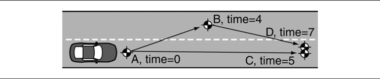
Figure 4.46: Different nodes with different times and the same position
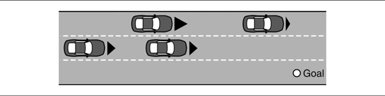
Figure 4.47: Navigating a gap through oncoming traffic
Incorporating time into the pathfinding graph allows us to rescue A* as our pathfinding algorithm for this problem.
The Size of the Graph
Unfortunately, we’ve only moved the problem along, not really solved it. Now we have not only an infinite number of places where we can change lanes but also (because of acceleration and braking) an infinite number of nodes representing every possible time for every possible place along the road. We now truly have a huge pathfinding graph, far too large to use efficiently.
We get around this problem by dynamically generating only the subsection of the graph that is actually relevant to the task. Figure 4.47 shows a simple case of the car dodging sideways through a gap in the oncoming traffic.
There are any number of ways to accomplish this. We can drive at full speed into the center lane as soon as possible and immediately out to the far side. We could brake, wait until the gap comes closer, and then pull into the gap. We could brake and wait for all the cars to go by. The options are endless.
We constrain the problem by using a heuristic. We make two assumptions: (1) if the car is to change lanes, it will do so as soon as possible; and (2) it will move in its current lane to its next lane change as quickly as possible.
The first assumption is sound. There are no situations in which changing lanes earlier rather than later will give the car less flexibility. The opposite is not true. Changing lanes at the last possible moment will often mean that opportunities are missed.
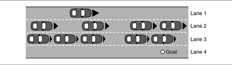
Figure 4.48: When top speed isn’t a good idea
The second assumption helps make sure the car is moving at top speed as much as possible. Unlike the first assumption, this may not be the best strategy. Figure 4.48 shows an extreme example.
Lane 4 is empty, but lanes 2 and 3 are both very busy. If the car streaks ahead to the front gap in lane 2, then it will not be able to cross into lane 3 and from there into lane 4. If it breaks, however, and waits until the second gap in lane 2 is aligned with the gap in lane 3, then it can streak through both gaps and onto the empty highway. In this case it pays to go slower initially.
In practice, such obvious pathological examples are rare. Drivers in a rush to get somewhere are quite likely to go as fast as they possibly can. Although it is not optimal, using this assumption produces AI drivers that behave plausibly: they don’t look like they are obviously missing simple opportunities.
How the Graph Is Created
The graph is created as is required by the pathfinding algorithm. Initially, the graph has only a single node in it: the current location of the AI police car, with the current time.
When the pathfinder asks for outgoing connections from the current node, the graph examines the cars on the road and returns four sets of connections.
First, it returns a connection to one node for each adjacent lane that is vacant at this point. I will call these nodes the lane change nodes. Their connection cost is the time required to change lanes at the current speed, and the destination nodes will have a position and a time value reflecting the lane change.
Second, the graph adds a connection to a node immediately behind the next car in the current lane, assuming that it travels as fast as possible and breaks at the very last minute to match the car’s speed (i.e., it doesn’t keep traveling at top speed and slam into the back of the car). The arrive and velocity match behaviors from Chapter 3 can calculate this kind of maneuver.
I will call this node the boundary node. If the AI cannot possibly avoid the collision (i.e., it can’t brake fast enough), then the boundary node is omitted; we don’t let the pathfinder even consider the possibility of crashing.
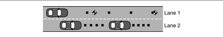
Figure 4.49: The placement of nodes within the same lane
Next, the graph returns connections to nodes along the current lane immediately after the AI passes each car in each adjacent lane, up until it reaches the next car in the current lane. For calculating these nodes assume that the car travels in the same way as we calculated for the boundary node; i.e., as fast as possible, making sure it doesn’t crash into the car in front. I will call these nodes safe opportunity nodes, because they represent the opportunity for the AI to change lanes, while making sure to avoid a collision with the car in front. Figure 4.49 shows this situation.
Because it is difficult to show time passing on a 2D graphic, I have indicated the position of each car in 1-second intervals as a black spot. Notice that the nodes in the current lane aren’t placed immediately after the current position of each car, but immediately after the position of each car when the AI would reach it.
Finally, the graph returns a set of unsafe opportunity nodes. These are exactly the same as the safe opportunity nodes, but are calculated assuming that the car always travels at top speed and doesn’t avoid slamming into the back of a car in front. These are useful because the pathfinder may choose to change lanes. There is no point in slowing down to avoid hitting a car in front if you intend to swerve around it into a different lane.
Notice that all four groups of connections are returned in the same set. They are all the connections outgoing from the current position of the police car; there is no distinction in the pathfinding algorithm. The connections and the nodes that they point to are created specially on this request.
The connections include a cost value. This is usually just a measure of time because we’re trying to move as quickly as possible. It would also be possible to include additional factors in the cost. A police driver might factor in how close each maneuver comes to colliding with an innocent motorist. Particularly close swerves would then only be used if they saved a lot of time.
The nodes referenced by each connection include both position information and time information.
As we’ve seen, we couldn’t hope to pre-create all nodes and connections, so they are built from scratch when the outgoing connections are requested from the graph.
On successive iterations of the pathfinding algorithm, the graph will be called again with a new start node. Since this node includes both a position and a time, we can predict where the cars on the road will be and repeat the process of generating connections.
Which Pathfinder
Two routes through the graph may end up at an identical node (i.e., one with the same position and timing information). In this case the connections leaving the node should be identical in every respect. In practice, this happens very rarely; the pathfinding graph tends to resemble a tree rather than a connected network.
Because it is rare to revisit a node that has already been visited, there is little point in storing a large number of nodes for future reference. Combined with the large size of the resulting graphs, a memory-saving variant of A* is the best choice. IDA* is unsuitable because retrieving the outgoing connections from a node is a very time-consuming process. IDA* replans through the same set of nodes at each iteration, incurring a significant performance hit. This could be mitigated by caching the connections from each node, but that goes against the memory-saving ethos of IDA*.
In my own experiments, SMA* seemed to be an excellent choice for pathfinding in this kind of continuous, dynamic task.
The remainder of this section is concerned with the dynamic graph algorithm only. The particular choice of pathfinder responsible for the planning is independent of the way the graph is implemented.
It is convenient to store driving actions in the connection data structure. When the final path is returned from the pathfinder, the driving AI will need to execute each maneuver. Each connection may have come from one of the four different categories, each of which involves a particular sequence of steering, acceleration, or breaking. There is no point in having to calculate this sequence again when it was calculated in the pathfinding graph. By storing it we can feed the action directly into the code that moves the car.
The algorithm is O(1) in memory, requiring only temporary storage. It is O(n) in time, where n is the number of vehicles in adjacent lanes, closer than the nearest vehicle in the current lane. The performance of the algorithm may be hampered by acquiring the data on adjacent cars. Depending on the data structure that stores the traffic pattern, this can be itself an O(log2 n) algorithm, where m is the number of cars in the lane (if it does a binary search for nearby cars, for example). By caching the results of the search each time, the practical performance can be brought back to O(n).
This algorithm is called at the lowest part of the pathfinding loop and therefore is highly speed critical.
Continuous pathfinding is a fairly complex algorithm to implement, and highly dependent on the situation. The example above is tied directly to the requirements of the car moving along the multi-lane road. Other kinds of movement may require different heuristics.
In practice, it can be extremely difficult to debug the placement of dynamic nodes. Especially so since nodes involving time are difficult to visualize.
Even when working properly, the algorithm is not fast, even in comparison with other pathfinders. It should probably be used for only small sections of planning. In the police driving game on which I’ve based this section, we used continuous planning to plan a route for only the next 100 yards or so. The remainder of the route was planned only on an intersectionby-intersection basis. The pathfinding system that drove the car was hierarchical, with the continuous planner being the lowest level of the hierarchy.
In the section on world representations, we looked briefly at situations where the orientation as well as the position of a character was used in planning. This helps to generate sensible paths for characters that cannot easily turn on the spot. In many cases pathfinding is used at a high level and doesn’t need to take account of these kinds of constraints; they will be handled by the steering behaviors. Increasingly, however, characters are highly constrained, and the steering behaviors discussed in the previous chapter cannot produce sensible results.
The first genre of game to show this inadequacy was urban driving. Vehicles such as cars or lorries need maneuver room and can often have lots of constraints specific to their physical capabilities (a car, for example, may need to decelerate before it can turn to avoid skidding).
Even non-driving game genres, in particular first- and third-person action games, are often set in highly constrained environments where steering alone cannot succeed. As animation fidelity has improved, characters need to move more fluidly through their environment. It is unacceptable for feet to intersect a staircase as if it were a ramp, or to slide when a character turns at low speed. Movement planning is a technique for using the algorithms in this chapter to produce sensible character movement: animation, steering, local and large-scale level navigation.
Most characters in a game have a range of animations that are used when the character is moving. A character may have a walk animation, a run animation, and a sprint animation, for example. Likewise, there are animations for turning—for example, turning while walking, turning on the spot, and turning while crouched.

Figure 4.50: Velocity diagram for allowed animations
Each of these animations can be used over a range of different movement scenarios. A walk animation, for example, needs to have the feet sticking to the ground and not sliding. So the character must move at a particular rate in order for the animation to look right. The speed of animation can be increased to accommodate slightly faster motion, but there are limits. Eventually, the character will look unbelievable.
It is possible to visualize animations as being applicable to a range of different movement speeds, both linear movement and angular movement. Figure 4.50 shows which animations can be used for different linear and angular velocities of a character.
Notice that not all the space of possible velocities has an associated animation. These are velocities that the character should not use for more than a moment.
In addition, it may not make sense to stop an animation before it has been completed. Most animation sets define transitions between walking and running and standing and crouching, for example. But a walk cycle may look odd being blended into a run cycle unless it has reached the right point for the transition to occur. This means that each movement has a natural length in the game world. Again, we can show this visually on a diagram. In this case, however, it is position and orientation shown, rather than velocity and rotation.
Notice in Figure 4.51 that the range over which the animations are believable is much smaller than for velocities.
It is possible to sidestep this problem entirely. Procedural animation, and human locomotion middleware is being applied to generating sensible animations for any movement required. It is not ubiquitous, however, and in many cases developers prefer motion captured or handmade animations. Most games still use a modest portfolio of possible animations, along with blending and parameterization.

Figure 4.51: Position diagram for allowed animations
In a highly constrained environment, the particular animations chosen may have a large impact on whether the character can maneuver correctly. A character that needs to move exactly 2 meters forward before doing a 30° right turn may not be able to use an animation that sends it 1.5 meters forward and rotates it by 45°.
To achieve a particular large-scale maneuver, the particular sequence of animations may be significant. In this case movement planning is required: planning a sequence of allowed maneuvers that lead to an overall state.
The Planning Graph
Just like pathfinding, movement planning uses a graph representation. In this case each node of the graph represents both the position and the state of the character at that point. A node may include the character’s position vector, its velocity vector, and the set of allowable animations that can follow. A running character, for example, may have high velocity and be capable of only carrying out the “run,” “transition run to walk,” or “collide with object” animations.
Connections in the graph represent valid animations; they lead to nodes representing the state of the character after the animation is complete. A run animation, for example, may lead to the character being 2 meters farther forward and traveling at the same velocity.
With the graph defined in this way, a heuristic can be used that determines how close a character’s state is to the goal. If the goal is to maneuver through a room full of exposed electrical wires, then the goal may be the door on the other side, and the heuristic may be based on distance alone. If the goal is to reach the edge of a platform traveling fast enough to jump a large gap, then the goal may include both position and velocity components.
Planning
With the graph defined in this way, the regular A* algorithm, or one of its siblings, can be used to plan a route. The route returned consists of a set of animations that, when executed in order, will move a character to its goal.
Care needs to be taken to define the goal in a broad way. If an exact position and orientation are given as a goal, then there may be no sequence of animations that exactly reach it, and the planning algorithm will fail (after considering every possible combination of animations, at a great cost of time). Rather, the goal needs to make sure the character is “near enough”; a range of states is allowable.
Infinite Graphs
Recall that an animation may be parameterized so that it can be used to travel a range of distances and through a range of velocities. Each possible distance and velocity would be a different state. So from one state the character may transition to any one of many similar states, depending on the speed it plays the following animation. If the velocities and positions are continuous (represented by real numbers), then there may be an infinite number of possible connections.
A* can be adapted to apply to infinite graphs. At each iteration of A*, all the successor nodes are examined using the heuristic function and added to the open list. To avoid this taking infinitely long, only the best successor nodes are returned for addition to the open list. This is often done by returning a few trial successors and then rating each heuristically. The algorithm can then try to generate a few more trials based on the best of the previous bunch, and so on until it is confident that the best successors have been provided. Although this technique is used in several non-game domains, it is slow and highly sensitive to the quality of the heuristic function.
To avoid the headaches involved in adapting A* to operate on infinite graphs, it is common to divide up the possible range into a small set of discrete values. If an animation can be played at between 15 and 30 frames per second (fps), then there may be four different possible values exposed to the planner: 15, 20, 25, and 30 fps.
Another alternative is to use domain-specific simplifying heuristics, as we saw in the previous section on continuous pathfinding. This allows us to dynamically generate a small subset of the pathfinding graph based on heuristics about what sections of the graph might be useful.

Figure 4.52: Example of an animation state machine
Implementation Issues
Even limiting the number of connections in this way, there are still a huge number of possible connections in the graph, and the graph tends to be very large indeed. The optimized versions of A* require us to know in advance the number of nodes in the graph. In movement planning the graph is usually generated on the fly: the successor nodes are generated by applying allowable animations to the current state. A basic, two list A* is therefore the most applicable for movement planning.
Typically, movement planning is only used for small sequences of movement. In the same way that the steering behavior of a character is guided by the large-scale pathfinding plan, movement planning can be used to fill in detail for just the next part of the overall route. If the plan states to move through a room with lots of live electrical wires, the movement planner may generate a sequence of animations to get to the other side only. It is unlikely to be used to generate a complete path through a level, because of the size of the graph involved and the planning time it would require.
As an example consider a walking bipedal character. The character has the following animations: walk, stand to walk, walk to stand, sidestep, and turn on the spot. Each animation starts or ends from one of two positions: mid-walk or standing still. The animation can be represented as the state machine in Figure 4.52, with the positions as states and the transitions as animations.
The animations can apply to the range of movement distances as shown on the graph in Figure 4.53.
The character is moving through the lava-filled room shown in Figure 4.54. There are many dangerous areas where the character should not walk. The character needs to work out a valid sequence of movements from its initial position to the opposite doorway. The goal is shown as a range of positions with no orientation. We don’t care what speed the character is traveling, which way it is facing, or what its animation state is when it reaches the goal.
Running an A*-style algorithm, we get the route generated in Figure 4.55. It can be seen that this avoids the dangers correctly using a combination of walking, turning, and sidestepping.

Figure 4.53: Example of position ranges for animations
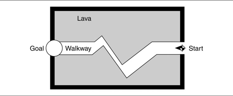
Figure 4.54: The dangerous room

Figure 4.55: The example path through the dangerous room
When movement planning is used to determine where character’s feet will be placed, it is called “footfall planning.” This is an active area of research in robotics, requiring the pathfinding system to have very fine data about the path of limbs in each animation. This is probably at too fine a level of detail for games.
Most recent third-person games lock footfalls correctly: particularly when climbing stairs, but also when navigating narrow ledges or avoiding ground clutter. As far as I know, the current state of the art uses purely local constraints to achieve this: the character’s footfall is examined and moved to the nearest suitable location, causing adjustments in the rest of the animation if required. This uses inverse kinematics algorithms for the animation, such algorithms are not normally associated with AI.
Footfall planning, on the other hand, would look ahead, using a series of animations to place footfalls in the correct locations to achieve a distant goal. As yet, I am not aware of anyone doing this.
EXERCISES
4.1 We can represent the graph in Figure 4.4 as a set of nodes and edges:
nodes = {A, B, C, D}
edges = {(A, B) : 4, (B, A) : 4, (A, D) : 5, (D, A) : 5,
(B, D) : 6, (D, B) : 6, (B, C) : 5, (C, B) : 5}.
The following description is of a weighted directed graph taken from an MIT lecture by Tomas Lozano-Perez and Leslie Kaelbling:
nodes = {S, A, B, C, D, G}
edges = {(S, A) : 6, (S, B) : 15, (A, C) : 6, (A, D) : 12,
(B, D) : 3, (B, G) : 15, (D, C) : 9, (D, G) : 6}.
Draw a diagram of the graph.
4.2 In the graph you drew in Exercise 4.1 assume that S is the start node and G is the goal node. If we use Dijkstra’s algorithm to find the minimum cost path from S to G, then the following table shows the contents of the open list for the first 2 steps of the algorithm. Fill in the remaining 5 lines.
Open List |
|
1 |
0: S |
2 |
6: A → S, 15: B → S |
3 |
|
4 |
|
5 |
|
6 |
|
7 |
4.3 In the answer to Exercise 4.2, explain why we don’t just stop when we visit the goal node for the first time.
4.4 For a node A, we can specify that the value of the heuristic function at the node is 5 by writing A : 5. Update the diagram you drew for Exercise 4.1 with the following heuristic values:
4.5 If the A* algorithm is applied to the same graph as in Exercise 4.2, the following table shows the contents of the open list for the first 2 steps. Fill in the remaining 3 lines.
Open List |
|
1 |
0:S |
2 |
12: A → S,24: B → S |
3 |
|
4 |
|
5 |
4.6 Using the same graph as for Exercise 4.5, what is the maximum value of the heuristic at D before the heuristic no longer underestimates the actual cost?
4.7 A heuristic is called consistent if it has the property that for every node A and every successor B of A, the estimated cost of reaching the goal from A is no greater than the cost of getting from A to B plus the estimated cost of reaching the goal from B. In equation form:
Is the heuristic defined in Exercise 4.4 consistent?
4.8 Explain why, if the heuristic used for A* is consistent and admissible, then you don’t need a closed list.
4.9 How could you make any admissible heuristic into a consistent one?
4.10 The grid below shows costs associated with cells on a map. For example, suppose the cells of cost 1 correspond to flat grassland while the cells of cost 3 correspond to more mountainous areas.

If we wanted to speed up A* would we artificially increase or decrease the costs of the mountainous areas? Why? What is the downside of making the change?
4.11 A common trick used in games to avoid the expense of taking square roots is to perform all distance comparisons with the distance squared. Explain why using the distance squared, in place of the standard Euclidean distance, as a heuristic for A* would be a bad idea.
4.12 For a world represented as a tile graph, where m is the cost to move between any two adjacent tiles, the Manhattan distance heuristic can be defined as:
Explain why this might be a better heuristic to use on a tile graph than the Euclidean distance.
4.13 Draw the navigation mesh you would get by considering edges as nodes in Figure 4.29.

Figure 4.56: A representation of a game level as a grid

Figure 4.57: Important points marked on part of a simple level
4.14 Games need to take into account many factors beside distance when calculating path costs. We’ll consider many examples in Chapter6, but try to think of some on your own in advance.
4.15 Compute the minimum, maximin, and average minimum distance costs of going from group B to group C in the tile-based representation of a level shown in Figure 4.56.
4.16 Figure 4.57 shows part of a level with 4 nodes, where S is the start, G is the goal, A is a node in a doorway, and B is a normal node. Nodes S, A, and G are all 3 units apart while B is 4 units from A.
Suppose for the door to open a character has to first stand in front of it for t seconds.
Assuming that a character moves at 1 unit per second, then for values of t = 1 and t = 7 draw a separate “nodes as states” graph like the one in Figure 4.46. For what value of t does it become faster to simply go around rather than wait for the door to open?