ONE of the most fundamental requirements of game AI is to sensibly move characters around. Even the earliest AI-controlled characters (the ghosts in Pac-Man, for example, or the opposing bat in some Pong variants) had movement algorithms that weren’t far removed from modern games.
Movement forms the lowest level of AI techniques in our model, shown in Figure 3.1.
Many games, including some with quite decent-looking AI, rely solely on movement algorithms and don’t have any more advanced decision making. At the other extreme, some games don’t need moving characters at all. Resource management games and turn-based games often don’t need movement algorithms; once a decision is made where to move, the character can simply be placed there.
There is also some degree of overlap between AI and animation; animation is also about movement. This chapter looks at large-scale movement: the movement of characters around the game level, rather than the movement of their limbs or faces. The dividing line isn’t always clear, however. In many games, animation can take control over a character, including some large-scale movement. This may be as simple as the character moving a few steps to pull a lever. Or as complex as mini cut-scenes, completely animated, that seamlessly transition into and out of gameplay. These are not AI driven and therefore aren’t covered here.
This chapter will look at a range of different AI-controlled movement algorithms, from the simple Pac-Man level up to the complex steering behaviors used for driving a racing car or piloting a spaceship in three dimensions.

Figure 3.1: The AI model
3.1 THE BASICS OF MOVEMENT ALGORITHMS
Unless you’re writing an economic simulator, chances are the characters in your game need to move around. Each character has a current position and possibly additional physical properties that control its movement. A movement algorithm is designed to use these properties to work out where the character should be next.
All movement algorithms have this same basic form. They take geometric data about their own state and the state of the world, and they come up with a geometric output representing the movement they would like to make. Figure 3.2 shows this schematically. In the figure, the velocity of a character is shown as optional because it is only needed for certain classes of movement algorithms.
Some movement algorithms require very little input: just the position of the character and the position of an enemy to chase, for example. Others require a lot of interaction with the game state and the level geometry. A movement algorithm that avoids bumping into walls, for example, needs to have access to the geometry of the wall to check for potential collisions.
The output can vary too. In most games it is normal to have movement algorithms output a desired velocity. A character might see its enemy to the west, for example, and respond that its movement should be westward at full speed. Often, characters in older games only had two speeds: stationary and running (with maybe a walk speed in there, too, for patrolling). So the output was simply a direction to move in. This is kinematic movement; it does not account for how characters accelerate and slow down.
It is common now for more physical properties to be taken into account. Producing movement algorithms I will call “steering behaviors.” Steering behaviors is the name given by Craig Reynolds to his movement algorithms [51]; they are not kinematic, but dynamic. Dynamic movement takes account of the current motion of the character. A dynamic algorithm typically needs to know the current velocities of the character as well as its position. A dynamic algorithm outputs forces or accelerations with the aim of changing the velocity of the character.
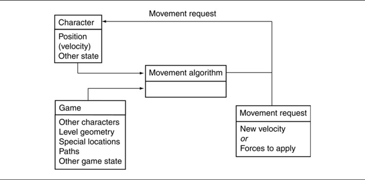
Figure 3.2: The movement algorithm structure
Dynamics adds an extra layer of complexity. Let’s say your character needs to move from one place to another. A kinematic algorithm simply gives the direction to the target; your character moves in that direction until it arrives, whereupon the algorithm returns no direction. A dynamic movement algorithm needs to work harder. It first needs to accelerate in the right direction, and then as it gets near its target it needs to accelerate in the opposite direction, so its speed decreases at precisely the correct rate to slow it to a stop at exactly the right place. Because Craig’s work is so well known, in the rest of this chapter I’ll usually follow the most common terminology and refer to all dynamic movement algorithms as steering behaviors.
Craig Reynolds also invented the flocking algorithm used in countless films and games to animate flocks of birds or herds of other animals. We’ll look at this algorithm later in the chapter. Because flocking is the most famous steering behavior, all steering algorithms (in fact, all movement algorithms) are sometimes wrongly called “flocking.”
3.1.1 TWO-DIMENSIONAL MOVEMENT
Many games have AI that works in two dimensions (2D). Even games that are rendered in three dimensions (3D), usually have characters that are under the influence of gravity, sticking them to the floor and constraining their movement to two dimensions.
A lot of movement AI can be achieved in 2D, and most of the classic algorithms are only defined for this case. Before looking at the algorithms themselves, we need to quickly cover the data needed to handle 2D math and movement.
Characters as Points
Although a character usually consists of a 3D model that occupies some space in the game world, many movement algorithms assume that the character can be treated as a single point. Collision detection, obstacle avoidance, and some other algorithms use the size of the character to influence their results, but movement itself assumes the character is at a single point. This is a process similar to that used by physics programmers who treat objects in the game as a “rigid body” located at its center of mass. Collision detection and other forces can be applied anywhere on the object, but the algorithm that determines the movement of the object converts them so it can deal only with the center of mass.
Characters in two dimensions have two linear coordinates representing the position of the object. These coordinates are relative to two world axes that lie perpendicular to the direction of gravity and perpendicular to each other. This set of reference axes is termed the orthonormal basis of the 2D space.
In most games the geometry is typically stored and rendered in three dimensions. The geometry of the model has a 3D orthonormal basis containing three axes: normally called x, y, and z. It is most common for the y-axis to be in the opposite direction to gravity (i.e., “up”) and for the x and z axes to lie in the plane of the ground. Movement of characters in the game takes place along the x and z axes used for rendering, as shown in Figure 3.3. For this reason this chapter will use the x and z axes when representing movement in two dimensions, even though books dedicated to 2D geometry tend to use x and y for the axis names.
In addition to the two linear coordinates, an object facing in any direction has one orientation value. The orientation value represents an angle from a reference axis. In our case we use a counterclockwise angle, in radians, from the positive z-axis. This is fairly standard in game engines; by default (i.e., with zero orientation a character is looking down the z-axis).
With these three values the static state of a character can be given in the level, as shown in Figure 3.4.
Algorithms or equations that manipulate this data are called static because the data do not contain any information about the movement of a character.
We can use a data structure of the form:
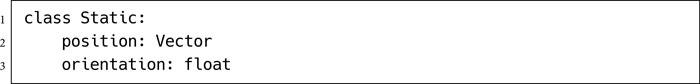

Figure 3.3: The 2D movement axes and the 3D basis
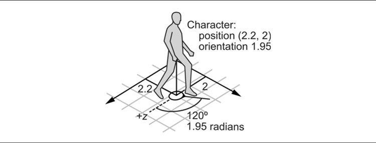
Figure 3.4: The positions of characters in the level
I will use the term orientation throughout this chapter to mean the direction in which a character is facing. When it comes to rendering characters, we will make them appear to face one direction by rotating them (using a rotation matrix). Because of this, some developers refer to orientation as rotation. I will use rotation in this chapter only to mean the process of changing orientation; it is an active process.
2½ Dimensions
Some of the math involved in 3D geometry is complicated. The linear movement in three dimensions is quite simple and a natural extension of 2D movement, but representing an orientation has tricky consequences that are better to avoid (at least until the end of the chapter).
As a compromise, developers often use a hybrid of 2D and 3D calculations which is known as 2½D, or sometimes four degrees of freedom.
In 2½ dimensions we deal with a full 3D position but represent orientation as a single value, as if we are in two dimensions. This is quite logical when you consider that most games involve characters under the influence of gravity. Most of the time a character’s third dimension is constrained because it is pulled to the ground. In contact with the ground, it is effectively operating in two dimensions, although jumping, dropping off ledges, and using elevators all involve movement through the third dimension.
Even when moving up and down, characters usually remain upright. There may be a slight tilt forward while walking or running or a lean sideways out from a wall, but this tilting doesn’t affect the movement of the character; it is primarily an animation effect. If a character remains upright, then the only component of its orientation we need to worry about is the rotation about the up direction.
This is precisely the situation we take advantage of when we work in 2½D, and the simplification in the math is worth the decreased flexibility in most cases.
Of course, if you are writing a flight simulator or a space shooter, then all the orientations are very important to the AI, so you’ll have to support the mathematics for three-dimensional orientation. At the other end of the scale, if your game world is completely flat and characters can’t jump or move vertically in any other way, then a strict 2D model is needed. In the vast majority of cases, 2½D is an optimal solution. I’ll cover full 3D motion at the end of the chapter, but aside from that, all the algorithms described in this chapter are designed to work in 2½D.
Math
In the remainder of this chapter I will assume that you are comfortable using basic vector and matrix mathematics (i.e., addition and subtraction of vectors, multiplication by a scalar). Explanations of vector and matrix mathematics, and their use in computer graphics, are beyond the scope of this book. If you can find it, the older book Schneider and Eberly [56], covers mathematical topics in computer games to a much deeper level. An excellent, and more recent alternative is [36].
Positions are represented as a vector with x and z components of position. In 2½D, a y component is also given.
In two dimensions we need only an angle to represent orientation. The angle is measured from the positive z-axis, in a right-handed direction about the positive y-axis (counterclockwise as you look down on the x–z plane from above). Figure 3.4 gives an example of how the scalar orientation is measured.
It is more convenient in many circumstances to use a vector representation of orientation. In this case the vector is a unit vector (it has a length of one) in the direction that the character is facing. This can be directly calculated from the scalar orientation using simple trigonometry:

Figure 3.5: The vector form of orientation
where ωs is the orientation as a scalar (i.e. a single number representing the angle), and is the orientation expressed as a vector. I am assuming a right-handed coordinate system here, in common with most of the game engines I’ve worked on,1 if you use a left-handed system, then simply flip the sign of the x coordinate:
If you draw the vector form of the orientation, it will be a unit length vector in the direction that the character is facing, as shown in Figure 3.5.
So far, each character has two associated pieces of information: its position and its orientation. We can create movement algorithms to calculate a target velocity based on position and orientation alone, allowing the output velocity to change instantly.
While this is fine for many games, it can look unrealistic. A consequence of Newton’s laws of motion is that velocities cannot change instantly in the real world. If a character is moving in one direction and then instantly changes direction or speed, it may look odd. To make smooth motion or to cope with characters that can’t accelerate very quickly, we need either to use some kind of smoothing algorithm or to take account of the current velocity and use accelerations to change it.
To support this, the character keeps track of its current velocity as well as position. Algorithms can then operate to change the velocity slightly at each frame, giving a smooth motion. Characters need to keep track of both their linear and their angular velocities. Linear velocity has both x and z components, the speed of the character in each of the axes in the orthonormal basis. If we are working in 2½D, then there will be three linear velocity components, in x, y, and z.
The angular velocity represents how fast the character’s orientation is changing. This is given by a single value: the number of radians per second that the orientation is changing.
I will call angular velocity rotation, since rotation suggests motion. Linear velocity will normally be referred to as simply velocity. We can therefore represent all the kinematic data for a character (i.e., its movement and position) in one structure:

Steering behaviors operate with these kinematic data. They return accelerations that will change the velocities of a character in order to move them around the level. Their output is a set of accelerations:

Independent Facing
Notice that there is nothing to connect the direction that a character is moving and the direction it is facing. A character can be oriented along the x-axis but be traveling directly along the z-axis. Most game characters should not behave in this way; they should orient themselves so they move in the direction they are facing.
Many steering behaviors ignore facing altogether. They operate directly on the linear components of the character’s data. In these cases the orientation should be updated so that it matches the direction of motion.
This can be achieved by directly setting the orientation to the direction of motion, but doing so may mean the orientation changes abruptly.
A better solution is to move it a proportion of the way toward the desired direction: to smooth the motion over many frames. In Figure 3.6, the character changes its orientation to be halfway toward its current direction of motion in each frame. The triangle indicates the orientation, and the gray shadows show where the character was in previous frames, to illustrate its motion.
Updating Position and Orientation
If your game uses a physics engine, it may be used to update the position and orientation of characters. Even with a physics engine, some developers prefer to use only its collision detection on characters, and code custom movement controllers. So if you need to update position and orientation manually, you can use a simple algorithm of the form:

Figure 3.6: Smoothing facing direction of motion over multiple frames

The updates use high-school physics equations for motion. If the frame rate is high, then the update time passed to this function is likely to be very small. The square of this time is likely to be even smaller, and so the contribution of acceleration to position and orientation will be tiny. It is more common to see these terms removed from the update algorithm, to give what’s known as the Newton-Euler-1 integration update:

This is the most common update used for games. Note that, in both blocks of code I’ve assumed that we can do normal mathematical operations with vectors, such as addition and multiplication by a scalar. Depending on the language you are using, you may have to replace these primitive operations with function calls.
The Game Physics [12] book in the Morgan Kaufmann Interactive 3D Technology series, and my Game Physics Engine Development [40], also in that series, have a complete analysis of different update methods and cover a more complete range of physics tools for games (as well as detailed implementations of vector and matrix operations).
Variable Frame Rates
So far I have assumed that velocities are given in units per second rather than per frame. Older games often used per-frame velocities, but that practice largely died out, before being resurrected occasionally when gameplay began to be processed in a separate execution thread with a fixed frame rate, separate to graphics updates (Unity’s FixedUpdate function compared to its variable Update, for example). Even with these functions available, it is more flexible to support variable frame rates, in case the fixed update rate needs changing. For this reason I will continue to use an explicit update time.
If the character is known to be moving at 1 meter per second and the last frame was of 20 milliseconds’ duration, then they will need to move 20 millimeters.
Forces and Actuation
In the real world we can’t simply apply an acceleration to an object and have it move. We apply forces, and the forces cause a change in the kinetic energy of the object. They will accelerate, of course, but the acceleration will depend on the inertia of the object. The inertia acts to resist the acceleration; with higher inertia, there is less acceleration for the same force.
To model this in a game, we could use the object’s mass for the linear inertia and the moment of inertia (or inertia tensor in three dimensions) for angular acceleration.
We could continue to extend the character data to keep track of these values and use a more complex update procedure to calculate the new velocities and positions. This is the method used by physics engines: the AI controls the motion of a character by applying forces to it. These forces represent the ways in which the character can affect its motion. Although not common for human characters, this approach is almost universal for controlling cars in driving games: the drive force of the engine and the forces associated with the steering wheels are the only ways in which the AI can control the movement of the car.
Because most well-established steering algorithms are defined with acceleration outputs, it is not common to use algorithms that work directly with forces. Usually, the movement controller considers the dynamics of the character in a post-processing step called actuation. Actuation takes as input a desired change in velocity, the kind that would be directly applied in a kinematic system. The actuator then calculates the combination of forces that it can apply to get as near as possible to the desired velocity change.
At the simplest level this is just a matter of multiplying the acceleration by the inertia to give a force. This assumes that the character is capable of applying any force, however, which isn’t always the case (a stationary car can’t accelerate sideways, for example). Actuation is a major topic in AI and physics integration, and I’ll return to actuation at some length in Section 3.8 of this chapter.
3.2 KINEMATIC MOVEMENT ALGORITHMS
Kinematic movement algorithms use static data (position and orientation, no velocities) and output a desired velocity. The output is often simply an on or off and a target direction, moving at full speed or being stationary. Kinematic algorithms do not use acceleration, although the abrupt changes in velocity might be smoothed over several frames.
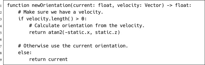
Many games simplify things even further and force the orientation of a character to be in the direction it is traveling. If the character is stationary, it faces either a pre-set direction or the last direction it was moving in. If its movement algorithm returns a target velocity, then that is used to set its orientation.
This can be done simply with the function:
We’ll look at two kinematic movement algorithms: seeking (with several of its variants) and wandering. Building kinematic movement algorithms is extremely simple, so we’ll only look at these two as representative samples before moving on to dynamic movement algorithms, the bulk of this chapter.
I can’t stress enough, however, that this brevity is not because they are uncommon or unimportant. Kinematic movement algorithms still form the bread and butter of movement systems in a lot of games. The dynamic algorithms in the rest of the book are widespread, where character movement is controlled by a physics engine, but they are still not ubiquitous.
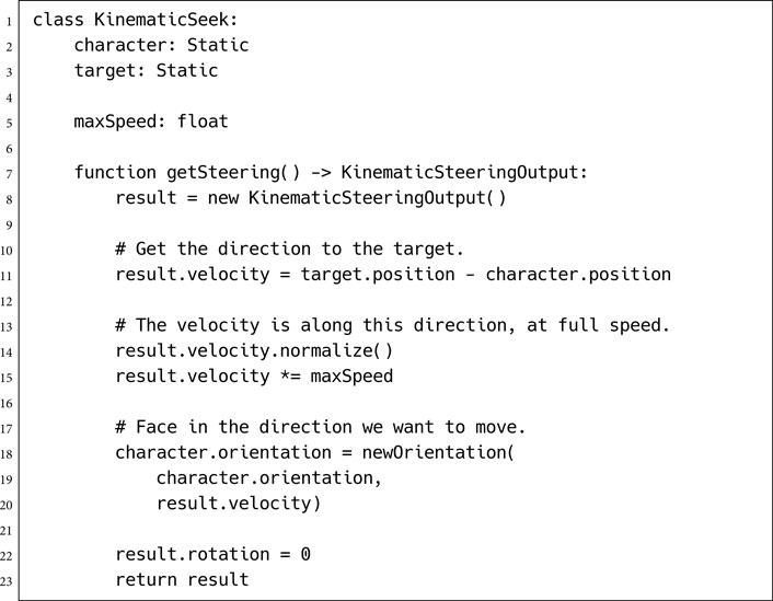
A kinematic seek behavior takes as input the character’s static data and its target’s static data. It calculates the direction from the character to the target and requests a velocity along this line. The orientation values are typically ignored, although we can use the newOrientation function above to face in the direction we are moving.
The algorithm can be implemented in a few lines:
where the normalize method applies to a vector and makes sure it has a length of one. If the vector is a zero vector, then it is left unchanged.
Data Structures and Interfaces
We use the Static data structure as defined at the start of the chapter and a KinematicSteeringOutput structure for output. The KinematicSteeringOutput structure has the following form:

In this algorithm rotation is never used; the character’s orientation is simply set based on their movement. You could remove the call to newOrientation if you want to control orientation independently somehow (to have the character aim at a target while moving, as in Tomb Raider [95], or twin-stick shooters such as The Binding of Isaac [151], for example).
Performance
The algorithm is O(1) in both time and memory.
Flee
If we want the character to run away from the target, we can simply reverse the second line of the getSteering method to give:

The character will then move at maximum velocity in the opposite direction.
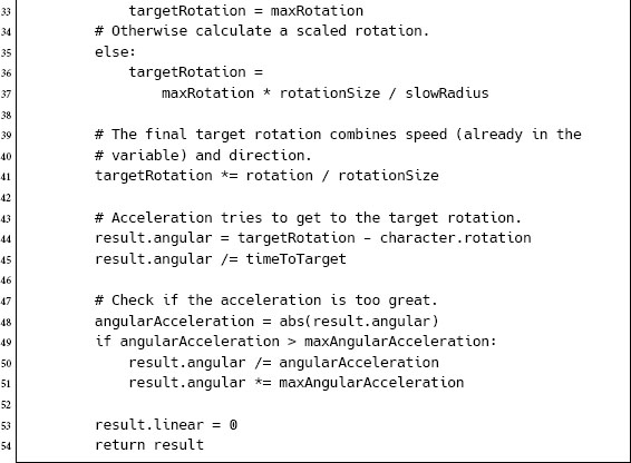
Arriving
The algorithm above is intended for use by a chasing character; it will never reach its goal, but it continues to seek. If the character is moving to a particular point in the game world, then this algorithm may cause problems. Because it always moves at full speed, it is likely to overshoot an exact spot and wiggle backward and forward on successive frames trying to get there. This characteristic wiggle looks unacceptable. We need to end by standing stationary at the target spot.
To achieve this we have two choices. We can just give the algorithm a large radius of satisfaction and have it be satisfied if it gets closer to its target than that. Alternatively, if we support a range of movement speeds, then we could slow the character down as it reaches its target, making it less likely to overshoot.
The second approach can still cause the characteristic wiggle, so we benefit from blending both approaches. Having the character slow down allows us to use a much smaller radius of satisfaction without getting wiggle and without the character appearing to stop instantly.
We can modify the seek algorithm to check if the character is within the radius. If so, it doesn’t worry about outputting anything. If it is not, then it tries to reach its target in a fixed length of time. (I’ve used a quarter of a second, which is a reasonable figure; you can tweak the value if you need to.) If this would mean moving faster than its maximum speed, then it moves at its maximum speed. The fixed time to target is a simple trick that makes the character slow down as it reaches its target. At 1 unit of distance away it wants to travel at 4 units per second. At a quarter of a unit of distance away it wants to travel at 1 unit per second, and so on. The fixed length of time can be adjusted to get the right effect. Higher values give a more gentle deceleration, and lower values make the braking more abrupt.
The algorithm now looks like the following:
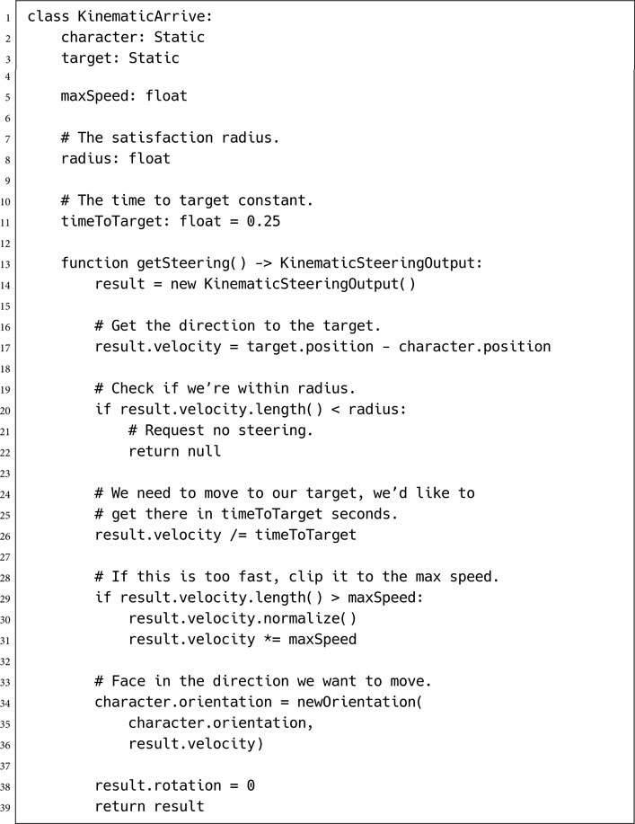
I’ve assumed a length function that gets the length of a vector.
A kinematic wander behavior always moves in the direction of the character’s current orientation with maximum speed. The steering behavior modifies the character’s orientation, which allows the character to meander as it moves forward. Figure 3.7 illustrates this. The character is shown at successive frames. Note that it moves only forward at each frame (i.e., in the direction it was facing at the previous frame).
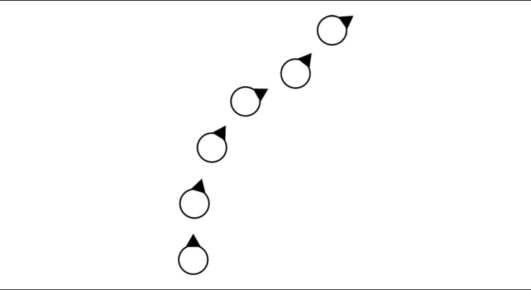
Figure 3.7: A character using kinematic wander
Pseudo-Code
It can be implemented as follows:
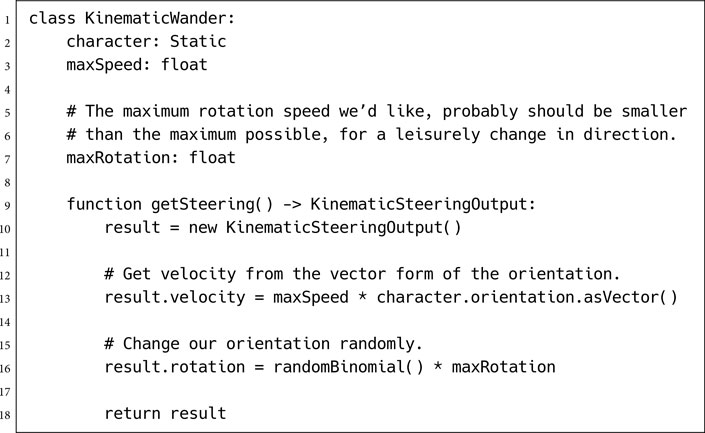
Data Structures
Orientation values have been given an asVector function that converts the orientation into a direction vector using the formulae given at the start of the chapter.
Implementation Notes
I’ve used randomBinomial to generate the output rotation. This is a handy random number function that isn’t common in the standard libraries of programming languages. It returns a random number between –1 and 1, where values around zero are more likely. It can be simply created as:

where random() returns a random number from 0 to 1.
For our wander behavior, this means that the character is most likely to keep moving in its current direction. Rapid changes of direction are less likely, but still possible.
Steering behaviors extend the movement algorithms in the previous section by adding velocity and rotation. In some genres (such as driving games) they are dominant; in other genres they are more context dependent: some characters need them, some characters don’t.
There is a whole range of different steering behaviors, often with confusing and conflicting names. As the field has developed, no clear naming schemes have emerged to tell the difference between one atomic steering behavior and a compound behavior combining several of them together.
In this book I’ll separate the two: fundamental behaviors and behaviors that can be built up from combinations of these.
There are a large number of named steering behaviors in various papers and code samples. Many of these are variations of one or two themes. Rather than catalog a zoo of suggested behaviors, we’ll look at the basic structures common to many of them before looking at some exceptions with unusual features.
By and large, most steering behaviors have a similar structure. They take as input the kinematic of the character that is moving and a limited amount of target information. The target information depends on the application. For chasing or evading behaviors, the target is often another moving character. Obstacle avoidance behaviors take a representation of the collision geometry of the world. It is also possible to specify a path as the target for a path following behavior.
The set of inputs to a steering behavior isn’t always available in an AI-friendly format. Collision avoidance behaviors, in particular, need to have access to collision information in the level. This can be an expensive process: checking the anticipated motion of the character using ray casts or trial movement through the level.
Many steering behaviors operate on a group of targets. The famous flocking behavior, for example, relies on being able to move toward the average position of the flock. In these behaviors some processing is needed to summarize the set of targets into something that the behavior can react to. This may involve averaging properties of the whole set (to find and aim for their center of mass, for example), or it may involve ordering or searching among them (such as moving away from the nearest predator or avoiding bumping into other characters that are on a collision course).
Notice that the steering behavior isn’t trying to do everything. There is no behavior to avoid obstacles while chasing a character and making detours via nearby power-ups. Each algorithm does a single thing and only takes the input needed to do that. To get more complicated behaviors, we will use algorithms to combine the steering behaviors and make them work together.
The simplest family of steering behaviors operates by variable matching: they try to match one or more of the elements of the character’s kinematic to a single target kinematic.
We might try to match the position of the target, for example, not caring about the other elements. This would involve accelerating toward the target position and decelerating once we are near. Alternatively, we could try to match the orientation of the target, rotating so that we align with it. We could even try to match the velocity of the target, following it on a parallel path and copying its movements but staying a fixed distance away.
Variable matching behaviors take two kinematics as input: the character kinematic and the target kinematic. Different named steering behaviors try to match a different combination of elements, as well as adding additional properties that control how the matching is performed.
It is possible, but not particularly helpful, to create a general steering behavior capable of matching any subset of variables and simply tell it which combination of elements to match. I’ve made the mistake of trying this implementation myself. The problem arises when more than one element of the kinematic is being matched at the same time. They can easily conflict. We can match a target’s position and orientation independently. But what about position and velocity? If we are matching velocities, between a character and its target, then we can’t simultaneously be trying to get any closer.
A better technique is to have individual matching algorithms for each element and then combine them in the right combination later. This allows us to use any of the steering behavior combination techniques in this chapter, rather than having one hard-coded. The algorithms for combing steering behaviors are designed to resolve conflicts and so are perfect for this task.
For each matching steering behavior, there is an opposite behavior that tries to get as far away from matching as possible. A behavior that tries to catch its target has an opposite that tries to avoid its target; a behavior that tries to avoid colliding with walls has an opposite that hugs them (perhaps for use in the character of a timid mouse) and so on. As we saw in the kinematic seek behavior, the opposite form is usually a simple tweak to the basic behavior. We will look at several steering behaviors in a pair with their opposite, rather than separating them into separate sections.
Seek tries to match the position of the character with the position of the target. Exactly as for the kinematic seek algorithm, it finds the direction to the target and heads toward it as fast as possible. Because the steering output is now an acceleration, it will accelerate as much as possible.
Obviously, if it keeps on accelerating, its speed will grow larger and larger. Most characters have a maximum speed they can travel; they can’t accelerate indefinitely. The maximum can be explicit, held in a variable or constant, or it might be a function of speed-dependent drag, slowing the character down more strongly the faster it goes.
With an explicit maximum, the current speed of the character (the length of the velocity vector) is checked regularly, and is trimmed back if it exceeds the maximum speed. This is normally done as a post-processing step of the update function. It is not normally performed in a steering behavior. For example,

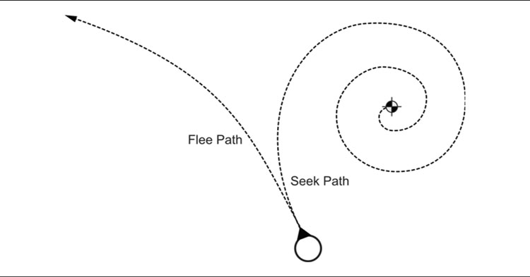
Figure 3.8: Seek and flee
Games that rely on physics engines typically include drag instead of a maximum speed (though they may use a maximum speed as well for safety). Without a maximum speed, the update does not need to check and clip the current velocity; the drag (applied in the physics update function) automatically limits the top speed.
Drag also helps another problem with this algorithm. Because the acceleration is always directed toward the target, if the target is moving, the seek behavior will end up orbiting rather than moving directly toward it. If there is drag in the system, then the orbit will become an inward spiral. If drag is sufficiently large, the player will not notice the spiral and will see the character simply move directly to its target.
Figure 3.8 illustrates the path that results from the seek behavior and its opposite, the flee path, described below.
Pseudo-Code
The dynamic seek implementation looks very similar to our kinematic version:

Note that I’ve removed the change in orientation that was included in the kinematic version. We can simply set the orientation, as we did before, but a more flexible approach is to use variable matching to make the character face in the correct direction. The align behavior, described below, gives us the tools to change orientation using angular acceleration. The “look where you’re going” behavior uses this to face the direction of movement.
Data Structures and Interfaces
This class uses the SteeringOutput structure we defined earlier in the chapter. It holds linear and angular acceleration outputs.
Performance
The algorithm is again O(1) in both time and memory.
Flee
Flee is the opposite of seek. It tries to get as far from the target as possible. Just as for kinematic flee, we simply need to flip the order of terms in the second line of the function:

The character will now move in the opposite direction of the target, accelerating as fast as possible.
Seek will always move toward its goal with the greatest possible acceleration. This is fine if the target is constantly moving and the character needs to give chase at full speed. If the character arrives at the target, it will overshoot, reverse, and oscillate through the target, or it will more likely orbit around the target without getting closer.
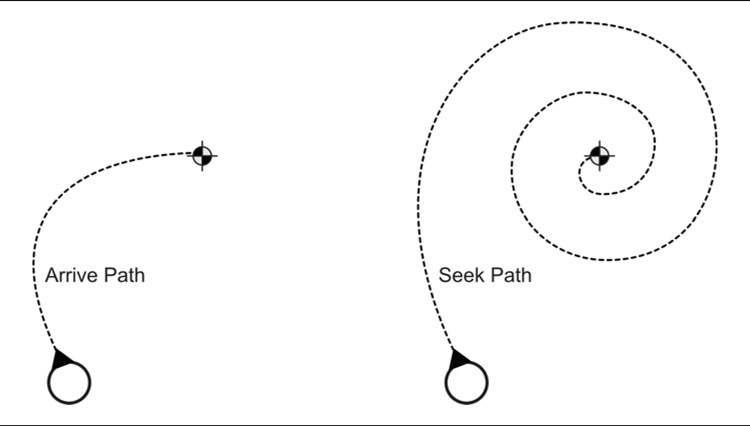
Figure 3.9: Seeking and arriving
If the character is supposed to arrive at the target, it needs to slow down so that it arrives exactly at the right location, just as we saw in the kinematic arrive algorithm. Figure 3.9 shows the behavior of each for a fixed target. The trails show the paths taken by seek and arrive. Arrive goes straight to its target, while seek orbits a bit and ends up oscillating. The oscillation is not as bad for dynamic seek as it was in kinematic seek: the character cannot change direction immediately, so it appears to wobble rather than shake around the target.
The dynamic arrive behavior is a little more complex than the kinematic version. It uses two radii. The arrival radius, as before, lets the character get near enough to the target without letting small errors keep it in motion. A second radius is also given, but is much larger. The incoming character will begin to slow down when it passes this radius. The algorithm calculates an ideal speed for the character. At the slowing-down radius, this is equal to its maximum speed. At the target point, it is zero (we want to have zero speed when we arrive). In between, the desired speed is an interpolated intermediate value, controlled by the distance from the target.
The direction toward the target is calculated as before. This is then combined with the desired speed to give a target velocity. The algorithm looks at the current velocity of the character and works out the acceleration needed to turn it into the target velocity. We can’t immediately change velocity, however, so the acceleration is calculated based on reaching the target velocity in a fixed time scale.
This is exactly the same process as for kinematic arrive, where we tried to get the character to arrive at its target in a quarter of a second. Because there is an extra layer of indirection (acceleration effects velocity which affects position) the fixed time period for dynamic arrive can usually be a little smaller; we’ll use 0.1 as a good starting point.
When a character is moving too fast to arrive at the right time, its target velocity will be smaller than its actual velocity, so the acceleration is in the opposite direction—it is acting to slow the character down.
Pseudo-Code
The full algorithm looks like the following:

Performance
The algorithm is O(1) in both time and memory, as before.
Implementation Notes
Many implementations do not use a target radius. Because the character will slow down to reach its target, there isn’t the same likelihood of oscillation that we saw in kinematic arrive. Removing the target radius usually makes no noticeable difference. It can be significant, however, with low frame rates or where characters have high maximum speeds and low accelerations. In general, it is good practice to give a margin of error around any target, to avoid annoying instabilities.
Leave
Conceptually, the opposite behavior of arrive is leave. There is no point in implementing it, however. If we need to leave a target, we are unlikely to want to accelerate with minuscule (possibly zero) acceleration first and then build up. We are more likely to accelerate as fast as possible. So for practical purposes the opposite of arrive is flee.
Align tries to match the orientation of the character with that of the target. It pays no attention to the position or velocity of the character or target. Recall that orientation is not directly related to direction of movement for a general kinematic. This steering behavior does not produce any linear acceleration; it only responds by turning.
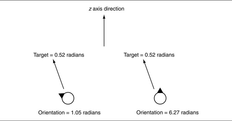
Figure 3.10: Aligning over a 2π radians boundary
Align behaves in a similar way to arrive. It tries to reach the target orientation and tries to have zero rotation when it gets there. Most of the code from arrive we can copy, but orientations have an added complexity that we need to consider.
Because orientations wrap around every 2π radians, we can’t simply subtract the target orientation from the character orientation and determine what rotation we need from the result. Figure 3.10 shows two very similar align situations, where the character is the same angle away from its target. If we simply subtracted the two angles, the first one would correctly rotate a small amount clockwise, but the second one would travel all around to get to the same place.
To find the actual direction of rotation, we subtract the character orientation from the target and convert the result into the range (−π, π) radians. We perform the conversion by adding or subtracting some multiple of 2π to bring the result into the given range. We can calculate the multiple to use by using the mod function and a little jiggling about. Most game engines or graphics libraries have one available (in Unreal Engine it is FMath::FindDeltaAngle, in Unity it is Mathf.DeltaAngle, though be aware that Unity uses degrees for its angles not radians).
We can then use the converted value to control rotation, and the algorithm looks very similar to arrive. Like arrive, we use two radii: one for slowing down and one to make orientations near the target acceptable. Because we are dealing with a single scalar value, rather than a 2D or 3D vector, the radius acts as an interval.
When we come to subtracting the rotation values, we have no problem we values repeating. Rotations, unlike orientations, don’t wrap: a rotation of π is not the same as a rotational of 3π. In fact we can have huge rotation values, well out of the (−π, π) range. Large values simply represent very fast rotation. Objects at very high speeds (such as the wheels in racing cars) may be rotating so fast that the updates we use here cause numeric instability. This is less of a problem on machines with 64-bit precision, but early physics on 32-bit machines often showed cars at high-speed having wheels that appeared to wobble. This has been resolved in robust physics engines, but it is worth knowing about, as the code we’re discussing here is basically implementing a simple physics update. The simple approach is effective for moderate rotational speeds.
Pseudo-Code
Most of the algorithm is similar to arrive, we simply add the conversion:

where the function abs returns the absolute (i.e., positive) value of a number; for example, –1 is mapped to 1.
Implementation Notes
Whereas in the arrive implementation there are two vector normalizations, in this code we need to normalize a scalar (i.e., turn it into either +1 or −1). To do this we use the result that:
![]()
In a production implementation in a language where you can access the bit pattern of a floating point number (C and C++, for example), you can do the same thing by manipulating the non-sign bits of the variable. Some C libraries provide an optimized sign function faster than the approach above.
Performance
The algorithm, unsurprisingly, is O(1) in both memory and time.
The Opposite
There is no such thing as the opposite of align. Because orientations wrap around every 2π, fleeing from an orientation in one direction will simply lead you back to where you started. To face the opposite direction of a target, simply add π to its orientation and align to that value.
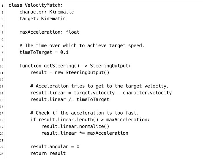
So far we have looked at behaviors that try to match position (linear position or orientation) with a target. We will do the same with velocity.
On its own this behavior is seldom used. It could be used to make a character mimic the motion of a target, but this isn’t very useful. Where it does become critical is when combined with other behaviors. It is one of the constituents of the flocking steering behavior, for example.
We have already implemented an algorithm that tries to match a velocity. Arrive calculates a target velocity based on the distance to its target. It then tries to achieve the target velocity. We can strip the arrive behavior down to provide a velocity matching implementation.
Pseudo-Code
The stripped down code looks like the following:
Performance
The algorithm is O(1) in both time and memory.
We have covered the basic building block behaviors that help to create many others. Seek and flee, arrive, and align perform the steering calculations for many other behaviors.
All the behaviors that follow have the same basic structure: they calculate a target, either a position or orientation (they could use velocity, but none of those we’re going to cover does), and then they delegate to one of the other behaviors to calculate the steering. The target calculation can be based on many inputs. Pursue, for example, calculates a target for seek based on the motion of another target. Collision avoidance creates a target for flee based on the proximity of an obstacle. And wander creates its own target that meanders around as it moves.
In fact, it turns out that seek, align, and velocity matching are the only fundamental behaviors (there is a rotation matching behavior, by analogy, but I’ve never seen an application for it). As we saw in the previous algorithm, arrive can be divided into the creation of a (velocity) target and the application of the velocity matching algorithm. This is common. Many of the delegated behaviors below can, in turn, be used as the basis of another delegated behavior. Arrive can be used as the basis of pursue, pursue can be used as the basis of other algorithms, and so on.
In the code that follows I will use a polymorphic style of programming to capture these dependencies. You could alternatively use delegation, having the primitive algorithms called by the new techniques. Both approaches have their problems. In our case, when one behavior extends another, it normally does so by calculating an alternative target. Using inheritance means we need to be able to change the target that the super-class works on.
If we use the delegation approach, we’d need to make sure that each delegated behavior has the correct character data, maxAcceleration, and other parameters. This requires duplication and data copying that using sub-classes removes.
So far we have moved based solely on position. If we are chasing a moving target, then constantly moving toward its current position will not be sufficient. By the time we reach where it is now, it will have moved. This isn’t too much of a problem when the target is close and we are reconsidering its location every frame. We’ll get there eventually. But if the character is a long distance from its target, it will set off in a visibly wrong direction, as shown in Figure 3.11.
Instead of aiming at its current position, we need to predict where it will be at some time in the future and aim toward that point. We did this naturally playing tag as children, which is why the most difficult tag players to catch were those who kept switching direction, foiling our predictions.
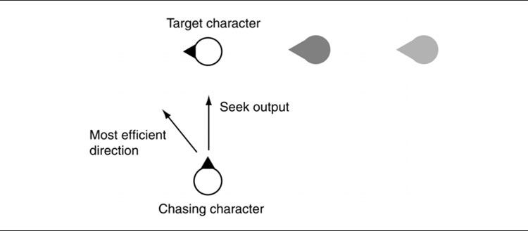
Figure 3.11: Seek moving in the wrong direction
We could use all kinds of algorithms to perform the prediction, but most would be overkill. Various research has been done into optimal prediction and optimal strategies for the character being chased (it is an active topic in military research for evading incoming missiles, for example). Craig Reynolds’s original approach is much simpler: we assume the target will continue moving with the same velocity it currently has. This is a reasonable assumption over short distances, and even over longer distances it doesn’t appear too stupid.
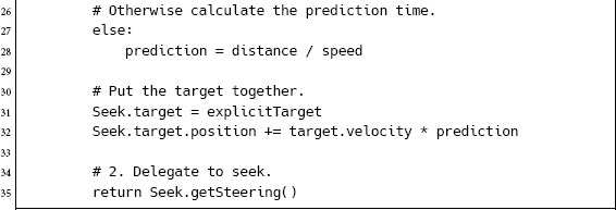
The algorithm works out the distance between character and target and works out how long it would take to get there, at maximum speed. It uses this time interval as its prediction lookahead. It calculates the position of the target if it continues to move with its current velocity. This new position is then used as the target of a standard seek behavior.
If the character is moving slowly, or the target is a long way away, the prediction time could be very large. The target is less likely to follow the same path forever, so we’d like to set a limit on how far ahead we aim. The algorithm has a maximum time parameter for this reason. If the prediction time is beyond this, then the maximum time is used.
Figure 3.12 shows a seek behavior and a pursue behavior chasing the same target. The pursue behavior is more effective in its pursuit.
Pseudo-Code
The pursue behavior derives from seek, calculates a surrogate target, and then delegates to seek to perform the steering calculation:

Figure 3.12: Seek and pursue

Implementation Notes
In this code I’ve used the slightly unsavory technique of naming a member variable in a derived class with the same name as the super-class. In most languages this will have the desired effect of creating two members with the same name. In our case this is what we want: setting the pursue behavior’s target will not change the target for the seek behavior it extends.
Be careful, though! In some languages (Python, for example) you can’t do this. You’ll have to name the target variable in each class with a different name.
As mentioned previously, it may be beneficial to cut out these polymorphic calls altogether to improve the performance of the algorithm. We can do this by having all the data we need in the pursue class, removing its inheritance of seek, and making sure that all the code the class needs is contained in the getSteering method. This is faster, but at the cost of duplicating the delegated code in each behavior that needs it and obscuring the natural reuse of the algorithm.
Performance
Once again, the algorithm is O(1) in both memory and time.
Evade
The opposite behavior of pursue is evade. Once again we calculate the predicted position of the target, but rather than delegating to seek, we delegate to flee.
In the code above, the class definition is modified so that it is a sub-class of Flee rather than Seek and thus Seek.getSteering is changed to Flee.getSteering.
Overshooting
If the chasing character is able to move faster than the target, it will overshoot and oscillate around its target, exactly as the normal seek behavior does.
To avoid this, we can replace the delegated call to seek with a call to arrive. This illustrates the power of building up behaviors from their logical components; when we need a slightly different effect, we can easily modify the code to get it.
The face behavior makes a character look at its target. It delegates to the align behavior to perform the rotation but calculates the target orientation first.
The target orientation is generated from the relative position of the target to the character.
It is the same process we used in the getOrientation function for kinematic movement.
Pseudo-Code
The implementation is very simple:

3.3.10 LOOKING WHERE YOU’RE GOING
So far, I have assumed that the direction a character is facing does not have to be its direction of motion. In many cases, however, we would like the character to face in the direction it is moving. In the kinematic movement algorithms we set it directly. Using the align behavior, we can give the character angular acceleration to make it face the correct direction. In this way the character changes facing gradually, which can look more natural, especially for aerial vehicles such as helicopters or hovercraft or for human characters that can move sideways (providing sidestep animations are available).
This is a process similar to the face behavior, above. The target orientation is calculated using the current velocity of the character. If there is no velocity, then the target orientation is set to the current orientation. We have no preference in this situation for any orientation.
Pseudo-Code
The implementation is even simpler than face:

Implementation Notes
In this case we don’t need another target member variable. There is no overall target; we are creating the current target from scratch. So, we can simply use Align.target for the calculated target (in the same way we did with pursue and the other derived algorithms).
Performance
The algorithm is O(1) in both memory and time.
The wander behavior controls a character moving aimlessly about.
When we looked at the kinematic wander behavior, we perturbed the wander direction by a random amount each time it was run. This makes the character move forward smoothly, but the rotation of the character is erratic, appearing to twitch from side to side as it moves.
The simplest wander approach would be to move in a random direction. This is unacceptable, and therefore almost never used, because it produces linear jerkiness. The kinematic version added a layer of indirection but produced rotational jerkiness. We can smooth this twitching by adding an extra layer, making the orientation of the character indirectly reliant on the random number generator.
We can think of kinematic wander as behaving as a delegated seek behavior. There is a circle around the character on which the target is constrained. Each time the behavior is run, we move the target around the circle a little, by a random amount. The character then seeks the target. Figure 3.13 illustrates this configuration.

Figure 3.13: The kinematic wander as a seek
We can improve this by moving the circle around which the target is constrained. If we move it out in front of the character (where front is determined by its current facing direction) and shrink it down, we get the situation in Figure 3.14.
The character tries to face the target in each frame, using the face behavior to align to the target. It then adds an extra step: applying full acceleration in the direction of its current orientation.
We could also implement the behavior by having it seek the target and perform a ‘look where you’re going’ behavior to correct its orientation.
In either case, the orientation of the character is retained between calls (so smoothing the changes in orientation). The angles that the edges of the circle subtend to the character determine how fast it will turn. If the target is on one of these extreme points, it will turn quickly. The target will twitch and jitter around the edge of the circle, but the character’s orientation will change smoothly.
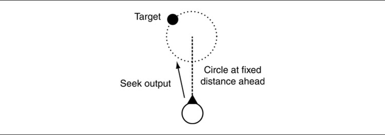
Figure 3.14: The full wander behavior
This wander behavior biases the character to turn (in either direction). The target will spend more time toward the edges of the circle, from the point of view of the character.
Pseudo-Code

Data Structures and Interfaces
I’ve used the same asVector function as earlier to get a vector form of the orientation.
Performance
The algorithm is O(1) in both memory and time.
So far we’ve seen behaviors that take a single target or no target at all. Path following is a steering behavior that takes a whole path as a target. A character with path following behavior should move along the path in one direction.
Path following, as it is usually implemented, is a delegated behavior. It calculates the position of a target based on the current character location and the shape of the path. It then hands its target off to seek. There is no need to use arrive, because the target should always be moving along the path. We shouldn’t need to worry about the character catching up with it.
The target position is calculated in two stages. First, the current character position is mapped to the nearest point along the path. This may be a complex process, especially if the path is curved or made up of many line segments. Second, a target is selected which is further along the path than the mapped point by some distance. To change the direction of motion along the path, we can change the sign of this distance. Figure 3.15 shows this in action. The current path location is shown, along with the target point a little way farther along. This approach is sometimes called “chase the rabbit,” after the way greyhounds chase the cloth rabbit at the dog track.

Figure 3.15: Path following behavior
Some implementations generate the target slightly differently. They first predict where the character will be in a short time and then map this to the nearest point on the path. This is a candidate target. If the new candidate target has not been placed farther along the path than it was at the last frame, then it is changed so that it is. I will call this predictive path following. It is shown in Figure 3.16. This latter implementation can appear smoother for complex paths with sudden changes of direction, but has the downside of cutting corners when two paths come close together.
Figure 3.17 shows this cutting-corner behavior. The character misses a whole section of the path. The character is shown at the instant its predictive future position crosses to a later part of the path.
This might not be what you want if, for example, the path represents a patrol route or a race track.
Pseudo-Code

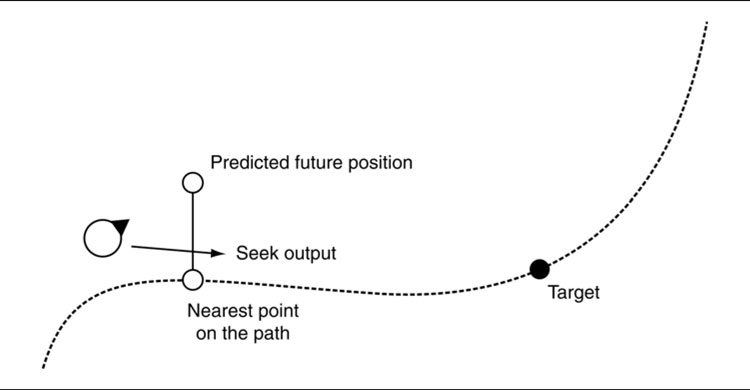
Figure 3.16: Predictive path following behavior
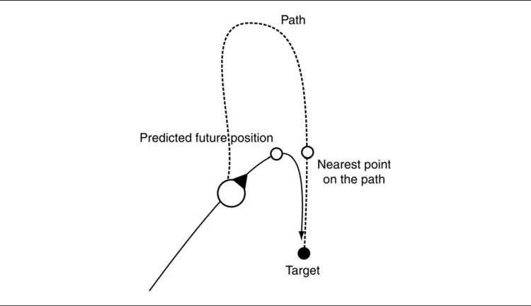
Figure 3.17: Vanilla and predictive path following
We can convert this algorithm to a predictive version by first calculating a surrogate position for the call to path.getParam. The algorithm looks almost identical:

Data Structures and Interfaces
The path that the behavior follows has the following interface:
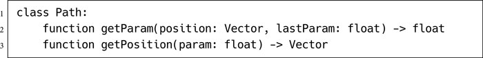
Both these functions use the concept of a path parameter. This is a unique value that increases monotonically along the path. It can be thought of as a distance along the path. Typically, paths are made up of line or curve splines; both of these are easily assigned parameters. The parameter allows us to translate between the position on the path and positions in 2D or 3D space.
Path Types
Performing this translation (i.e., implementing a path class) can be tricky, depending on the format of the path used.
It is most common to use a path of straight line segments as shown in Figure 3.18. In this case the conversion is not too difficult. We can implement getParam by looking at each line segment in turn, determining which one the character is nearest to, and then finding the nearest point on that segment. For smooth curved splines common in some driving games, however, the math can be more complex. A good source for closest-point algorithms for a range of different geometries is Schneider and Eberly [56].
Keeping Track of the Parameter
The pseudo-code interface above provides for sending the last parameter value to the path in order to calculate the current parameter value. This is essential to avoid nasty problems when lines are close together.
We limit the getParam algorithm to only considering areas of the path close to the previous parameter value. The character is unlikely to have moved far, after all. This technique, assuming the new value is close to the old one, is called coherence, and it is a feature of many geometric algorithms. Figure 3.19 shows a problem that would fox a non-coherent path follower but is easily handled by assuming the new parameter is close to the old one.
Of course, you may really want corners to be cut or a character to move between very different parts of the path. If another behavior interrupts and takes the character across the level, for example, you don’t necessarily want it to come all the way back to pick up a circular patrol route. In this case, you’ll need to remove coherence or at least widen the range of parameters that it searches for a solution.
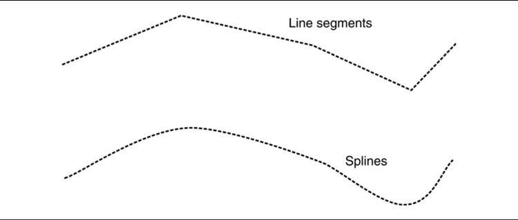
Figure 3.18: Path types

Figure 3.19: Coherence problems with path following
Performance
The algorithm is O(1) in both memory and time. The getParam function of the path will usually be O(1), although it may be O(n), where n is the number of segments in the path. If this is the case, then the getParam function will dominate the performance scaling of the algorithm.
The separation behavior is common in crowd simulations, where a number of characters are all heading in roughly the same direction. It acts to keep the characters from getting too close and being crowded.
It doesn’t work as well when characters are moving across each other’s paths. The collision avoidance behavior, below, should be used in this case.
Most of the time, the separation behavior has a zero output; it doesn’t recommend any movement at all. If the behavior detects another character closer than some threshold, it acts in a way similar to an evade behavior to move away from the character. Unlike the basic evade behavior, however, the strength of the movement is related to the distance from the target. The separation strength can decrease according to any formula, but a linear or an inverse square law decay is common.
Linear separation looks like the following:
![]()
The inverse square law looks like the following:
![]()
In each case, distance is the distance between the character and its nearby neighbor, threshold is the minimum distance at which any separation output occurs, and maxAcceleration is the maximum acceleration of the character. The k constant can be set to any positive value. It controls how fast the separation strength decays with distance.
Separation is sometimes called the “repulsion” steering behavior, because it acts in the same way as a physical repulsive force (an inverse square law force such as magnetic repulsion).
Where there are multiple characters within the avoidance threshold, either the closest can be selected, or the steering can be calculated for each in turn and summed. In the latter case, the final value may be greater than the maxAcceleration, in which case it should be clipped to that value.
Pseudo-Code

Implementation Notes
In the algorithm above, we simply look at each possible character in turn and work out whether we need to separate from them. For a small number of characters, this will be the fastest approach. For a few hundred characters in a level, we need a faster method.
Typically, graphics and physics engines rely on techniques to determine what objects are close to one another. Objects are stored in spatial data structures, so it is relatively easy to make this kind of query. Multi-resolution maps, quad-or octrees, and binary space partition (BSP) trees are all popular data structures for rapidly calculating potential collisions. Each of these can be used by the AI to get potential targets more efficiently.
Implementing a spatial data structure for collision detection is beyond the scope of this book. Other books in this series cover the topic in much more detail, particularly Ericson [14] and van den Bergen [73].
Performance
The algorithm is O(1) in memory and O(n) in time, where n is the number of potential targets to check. If there is some efficient way of pruning potential targets before they reach the algorithm above, the overall performance in time will improve. A BSP system, for example, can give O(log n) time, where n is the total number of potential targets in the game. The algorithm above will always remain linear in the number of potential targets it checks, however.
Attraction
Using the inverse square law, we can set a negative value for the constant of decay and get an attractive force. The character will be attracted to others within its radius. This works, but is rarely useful.
Some developers have experimented with having lots of attractors and repulsors in their level and having character movement mostly controlled by these. Characters are attracted to their goals and repelled from obstacles, for example. Despite being ostensibly simple, this approach is full of traps for the unwary.
The next section, on combining steering behaviors, shows why simply having lots of attractors or repulsors leads to characters that regularly get stuck and why starting with a more complex algorithm ends up being less work in the long run.
Independence
The separation behavior isn’t much use on its own. Characters will jiggle out of separation, but then never move again. Separation, along with the remaining behaviors in this chapter, is designed to work in combination with other steering behaviors. We return to how this combination works in the next section.

Figure 3.20: Separation cones for collision avoidance
In urban areas, it is common to have large numbers of characters moving around the same space. These characters have trajectories that cross each other, and they need to avoid constant collisions with other moving characters.
A simple approach is to use a variation of the evade or separation behavior, which only engages if the target is within a cone in front of the character. Figure 3.20 shows a cone that has another character inside it.
The cone check can be carried out using a dot product:

where direction is the direction between the behavior’s character and the potential collision. The coneThreshold value is the cosine of the cone half-angle, as shown in Figure 3.20.
If there are several characters in the cone, then the behavior needs to avoid them all. We can approach this in a similar way to the separation behavior. It is often sufficient to find the average position and speed of all characters in the cone and evade that target. Alternatively, the closest character in the cone can be found and the rest ignored.
Unfortunately, this approach, while simple to implement, doesn’t work well with more than a handful of characters. The character does not take into account whether it will actually collide but instead has a “panic” reaction to even coming close. Figure 3.21 shows a simple situation where the character will never collide, but our naive collision avoidance approach will still take action.
Figure 3.22 shows another problem situation. Here the characters will collide, but neither will take evasive action because they will not have the other in their cone until the moment of collision.

Figure 3.21: Two in-cone characters who will not collide

Figure 3.22: Two out-of-cone characters who will collide
A better solution works out whether or not the characters will collide if they keep to their current velocity. This involves working out the closest approach of the two characters and determining if the distance at this point is less than some threshold radius. This is illustrated in Figure 3.23.
Note that the closest approach will not normally be the same as the point where the future trajectories cross. The characters may be moving at very different velocities, and so are likely to reach the same point at different times. We simply can’t see if their paths will cross to check if the characters will collide. Instead, we have to find the moment that they are at their closest, use this to derive their separation, and check if they collide.
The time of closest approach is given by

Figure 3.23: Collision avoidance using collision prediction
where dp is the current relative position of target to character (what we called the distance vector from previous behaviors):
and dv is the relative velocity:
If the time of closest approach is negative, then the character is already moving away from the target, and no action needs to be taken.
From this time, the position of character and target at the time of closest approach can be calculated:
We then use these positions as the basis of an evade behavior; we are performing an evasion based on our predicted future positions, rather than our current positions. In other words, the behavior makes the steering correction now, as if it were already at the most compromised position it will get to.
For a real implementation it is worth checking if the character and target are already in collision. In this case, action can be taken immediately, without going through the calculations to work out if they will collide at some time in the future. In addition, this approach will not return a sensible result if the centers of the character and target will collide at some point. A sensible implementation will have some special case code for this unlikely situation to make sure that the characters will sidestep in different directions. This can be as simple as falling back to the evade behavior on the current positions of the character.
For avoiding groups of characters, averaging positions and velocities do not work well with this approach. Instead, the algorithm needs to search for the character whose closest approach will occur first and to react to this character only. Once this imminent collision is avoided, the steering behavior can then react to more distant characters.
Pseudo-Code

Performance
The algorithm is O(1) in memory and O(n) in time, where n is the number of potential targets to check.
As in the previous algorithm, if there is some efficient way of pruning potential targets before they reach the algorithm above, the overall performance in time will improve. This algorithm will always remain linear in the number of potential targets it checks, however.
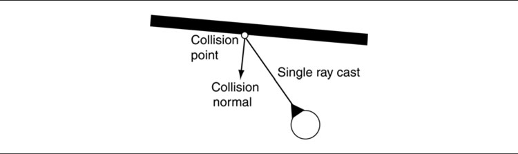
Figure 3.24: Collision ray avoiding a wall
3.3.15 OBSTACLE AND WALL AVOIDANCE
The collision avoidance behavior assumes that targets are spherical. It is interested in avoiding a trajectory too close to the center point of the target.
This can also be applied to any obstacle in the game that is easily represented by a bounding sphere. Crates, barrels, and small objects can be avoided simply this way.
More complex obstacles cannot be easily represented as circles. The bounding sphere of a large object, such as a staircase, can fill a room. We certainly don’t want characters sticking to the outside of the room just to avoid a staircase in the corner. By far the most common obstacles in the game are walls, and they cannot be simply represented by bounding spheres at all.
The obstacle and wall avoidance behavior uses a different approach to avoiding collisions. The moving character casts one or more rays out in the direction of its motion. If these rays collide with an obstacle, then a target is created that will avoid the collision, and the character does a basic seek on this target. Typically, the rays are not infinite. They extend a short distance ahead of the character (usually a distance corresponding to a few seconds of movement).
Figure 3.24 shows a character casting a single ray that collides with a wall. The point and normal of the collision with the wall are used to create a target location at a fixed distance from the surface.
Pseudo-Code

Data Structures and Interfaces
The collision detector has the following interface:

where getCollision returns the first collision for the character if it begins at the given position and moves by the given movement amount. Collisions in the same direction, but farther than moveAmount, are ignored.
Typically, this call is implemented by casting a ray from position to position + moveAmount and checking for intersections with walls or other obstacles.
The getCollision method returns a collision data structure of the form:

where position is the collision point and normal is the normal of the wall at the point of collision. These are standard data to expect from a collision detection routine, and most engines provide such data as a matter of course (see Physics.Raycast in Unity, in Unreal Engine it requires more setup, see the documentation for Traces).

Figure 3.25: Grazing a wall with a single ray and avoiding it with three
Performance
The algorithm is O(1) in both time and memory, excluding the performance of the collision detector (or rather, assuming that the collision detector is O(1)). In reality, collision detection using ray casts is quite expensive and is almost certainly not O(1) (it normally depends on the complexity of the environment). You should expect that most of the time spent in this algorithm will be spent in the collision detection routine.
Collision Detection Problems
So far we have assumed that we are detecting collisions with a single ray cast. In practice, this isn’t a good solution.
Figure 3.25 shows a one-ray character colliding with a wall that it never detects. Typically, a character will need to have two or more rays. The figure shows a three-ray character, with the rays splayed out to act like whiskers. This character will not graze the wall.
I have seen several basic ray configurations used over and over for wall avoidance. Figure 3.26 illustrates these.
There are no hard and fast rules as to which configuration is better. Each has its own particular idiosyncrasies. A single ray with short whiskers is often the best initial configuration to try but can make it impossible for the character to move down tight passages. The single ray configuration is useful in concave environments but grazes convex obstacles. The parallel configuration works well in areas where corners are highly obtuse but is very susceptible to the corner trap, as we’ll see.

Figure 3.26: Ray configurations for obstacle avoidance

Figure 3.27: The corner trap for multiple rays
The Corner Trap
The basic algorithm for multi-ray wall avoidance can suffer from a crippling problem with acute angled corners (any convex corner, in fact, but it is more prevalent with acute angles). Figure 3.27 illustrates a trapped character. Currently, its left ray is colliding with the wall. The steering behavior will therefore turn it to the left to avoid the collision. Immediately, the right ray will then be colliding, and the steering behavior will turn the character to the right.
When the character is run in the game, it will appear to home into the corner directly, until it slams into the wall. It will be unable to free itself from the trap.
The fan structure, with a wide enough fan angle, alleviates this problem. Often, there is a trade-off, however, between avoiding the corner trap with a large fan angle and keeping the angle small to allow the character to access small passageways. At worst, with a fan angle near π radians, the character will not be able to respond quickly enough to collisions detected on its side rays and will still graze against walls.

Figure 3.28: Collision detection with projected volumes
Several developers have experimented with adaptive fan angles. If the character is moving successfully without a collision, then the fan angle is narrowed. If a collision is detected, then the fan angle is widened. If the character detects many collisions on successive frames, then the fan angle will continue to widen, reducing the chance that the character is trapped in a corner.
Other developers implement specific corner-trap avoidance code. If a corner trap is detected, then one of the rays is considered to have won, and the collisions detected by other rays are ignored for a while.
Both approaches work well and represent practical solutions to the problem. The only complete solution, however, is to perform the collision detection using a projected volume rather than a ray, as shown in Figure 3.28.
Many game engines are capable of doing this, for the sake of modeling realistic physics. Unlike for AI, the projection distances required by physics are typically very small, however, and the calculations can be very slow when used in a steering behavior.
In addition, there are complexities involved in interpreting the collision data returned from a volume query. Unlike for physics, it is not the first collision point that needs to be considered (this could be the edge of a polygon on one extreme of the character model), but how the overall character should react to the wall. So far there is no widely trusted mechanism for doing volume prediction in wall avoidance.
For now, it seems that the most practical solution is to use adaptive fan angles, with one long ray cast and two shorter whiskers.

Figure 3.29: Steering family tree
Figure 3.29 shows a family tree of the steering behaviors we have looked at in this section. We’ve marked a steering behavior as a child of another if it can be seen as extending the behavior of its parent.
3.4 COMBINING STEERING BEHAVIORS
Individually, steering behaviors can achieve a good degree of movement sophistication. In many games steering simply consists of moving toward a given location: the seek behavior.
Higher level decision making tools are responsible for determining where the character intends to move. This is often a pathfinding algorithm, generating intermediate targets on the path to a final goal.
This only gets us so far, however. A moving character usually needs more than one steering behavior. It needs to reach its goal, avoid collisions with other characters, tend toward safety as it moves, and avoid bumping into walls. Wall and obstacle avoidance can be particularly difficult to get when working with other behaviors. In addition, some complex steering, such as flocking and formation motion, can only be accomplished when more than one steering behavior is active at once.
This section looks at increasingly sophisticated ways of accomplishing this combination: from simple blending of steering outputs to complicated pipeline architectures designed explicitly to support collision avoidance.
3.4.1 BLENDING AND ARBITRATION
By combining steering behaviors together, more complex movement can be achieved. There are two methods of combining steering behaviors: blending and arbitration.
Each method takes a portfolio of steering behaviors, each with its own output, and generates a single overall steering output. Blending does this by executing all the steering behaviors and combining their results using some set of weights or priorities. This is sufficient to achieve some very complex behaviors, but problems arise when there are a lot of constraints on how a character can move. Arbitration selects one or more steering behaviors to have complete control over the character. There are many arbitration schemes that control which behavior gets to have its way.
Blending and arbitration are not exclusive approaches, however. They are the ends of a continuum.
Blending may have weights or priorities that change over time. Some process needs to change these weights, and this might be in response to the game situation or the internal state of the character. The weights used for some steering behaviors may be zero; they are effectively switched off.
At the same time, there is nothing that requires an arbitration architecture to return a single steering behavior to execute. It may return a set of blending weights for combining a set of different behaviors.
A general steering system needs to combine elements of both blending and arbitration. Although we’ll look at different algorithms for each, an ideal implementation will mix elements of both.
The simplest way to combine steering behaviors is to blend their results together using weights.
Suppose we have a crowd of rioting characters in our game. The characters need to move as a mass, while making sure that they aren’t consistently bumping into each other. Each character needs to stay by the others, while keeping a safe distance. Their overall behavior is a blend of two behaviors: arriving at the center of mass of the group and separation from nearby characters. At no point is the character doing just one thing. It is always taking both concerns into consideration.

Figure 3.30: Blending steering outputs
The Algorithm
A group of steering behaviors can be blended together to act as a single behavior. Each steering behavior in the portfolio is asked for its acceleration request, as if it were the only behavior operating.
These accelerations are combined together using a weighted linear sum, with coefficients specific to each behavior. There are no constraints on the blending weights; they don’t have to sum to one, for example, and rarely do (i.e., it isn’t a weighted mean).
The final acceleration from the sum may be too great for the capabilities of the character, so it is trimmed according to the maximum possible acceleration (a more complex actuation step can always be used; see Section 3.8 on motor control later in the chapter).
In our crowd example, we may use weights of 1 for both separation and cohesion. In this case the requested accelerations are summed and cropped to the maximum possible acceleration. This is the output of the algorithm. Figure 3.30 illustrates this process.
As in all parameterized systems, the choice of weights needs to be the subject of inspired guesswork or good trial and error. Research projects have tried to evolve the steering weights using genetic algorithms or neural networks. Results have not been encouraging, however, and manual experimentation still seems to be the most sensible approach.
Pseudo-Code
The algorithm for blended steering is as follows:
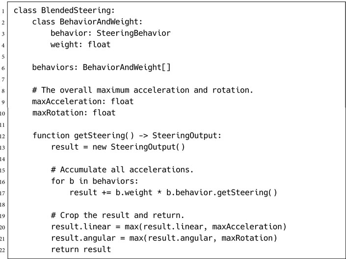
Data Structures
I have assumed that instances of the SteeringOutput structure can be added together and multiplied by a scalar. In each case these operations should be performed component-wise (i.e., linear and angular components should individually be added and multiplied).
Performance
The algorithm requires only temporary storage for the acceleration. It is O(1) in memory. It is O(n) for time, where n is the number of steering behaviors in the list. The practical execution speed of this algorithm depends on the efficiency of the component steering behaviors.
Flocking and Swarming
The original research into steering behaviors by Craig Reynolds modeled the movement patterns of flocks of simulated birds (known as “boids”). Though not the most commonly implemented in a game, flocking is the most commonly cited steering behavior. It relies on a simple weighted blend of simpler behaviors.
It is so ubiquitous that all steering behaviors are sometimes referred to, incorrectly, as “flocking.” I’ve even seen AI programmers fall into this habit at times.
The flocking algorithm relies on blending three simple steering behaviors: move away from boids that are too close (separation), move in the same direction and at the same velocity as the flock (alignment and velocity matching), and move toward the center of mass of the flock (cohesion). The cohesion steering behavior calculates its target by working out the center of mass of the flock. It then hands off this target to a regular arrive behavior.
For simple flocking, using equal weights may be sufficient. To get a more biologically believable behavior, however, separation is more important than cohesion, which is more important than alignment. The latter two are sometimes seen reversed.

Figure 3.31: The three components of flocking behaviors

Figure 3.32: The neighborhood of a boid
These behaviors are shown schematically in Figure 3.31.
In most implementations the flocking behavior is modified to ignore distant boids. In each behavior there is a neighborhood in which other boids are considered. Separation only avoids nearby boids; cohesion and alignment calculate and seek the position, facing, and velocity of only neighboring boids. The neighborhood is most commonly a simple radius, although Reynolds suggests it should have an angular cut-off, as shown in Figure 3.32.