7

LEARNING

MACHINE LEARNING (often abbreviated ML, though in this book I will simply call it ‘learning’) is a hot topic in technology and business, and that excitement has filtered into games. In principle, learning AI has the potential to adapt to each player, learning their tricks and techniques and providing a consistent challenge. It has the potential to produce more believable characters: characters that can learn about their environment and use it to the best effect. It also has the potential to reduce the effort needed to create game-specific AI: characters should be able to learn about their surroundings and the tactical options that they provide.

In practice, it hasn’t yet fulfilled its promise, and not for want of trying. Applying learning to your game requires careful planning and an understanding of the pitfalls. There have been some impressive successes in building learning AI that learns to play games, but less in providing compelling characters or enemies. The potential is sometimes more attractive than the reality, but if you understand the quirks of each technique and are realistic about how you apply them, there is no reason why you can’t take advantage of learning in your game.

There is a whole range of different learning techniques, from very simple number tweaking through to complex neural networks. While most of the attention in the last few years has been focused on ‘deep learning’ (a form of neural networks) there are many other practical approaches. Each has its own idiosyncrasies that need to be understood before they can be used in real games.

7.1  LEARNING BASICS

We can classify learning techniques into several groups depending on when the learning occurs, what is being learned, and what effects the learning has on a character’s behavior.

7.1.1  ONLINE OR OFFLINE LEARNING

Learning can be performed during the game, while the player is playing. This is online learning, and it allows the characters to adapt dynamically to the player’s style and provides more consistent challenges. As a player plays more, their characteristic traits can be better anticipated by the computer, and the behavior of characters can be tuned to playing styles. This might be used to make enemies pose an ongoing challenge, or it could be used to offer the player more story lines of the kind they enjoy playing.

Unfortunately, online learning also produces problems with predictability and testing. If the game is constantly changing, it can be difficult to replicate bugs and problems. If an enemy character decides that the best way to tackle the player is to run into a wall, then it can be a nightmare to replicate the behavior (at worst you’d have to play through the whole same sequence of games, doing exactly the same thing each time as the player). I’ll return to this issue later in this section.

The majority of learning in game AI is done offline, either between levels of the game or more often at the development studio before the game leaves the building. This is performed by processing data about real games and trying to calculate strategies or parameters from them.

This allows more unpredictable learning algorithms to be tried out and their results to be tested exhaustively. The learning algorithms in games are usually applied offline; it is rare to find games that use any kind of online learning. Learning algorithms are increasingly being used offline to learn tactical features of multi-player maps, to produce accurate pathfinding and movement data, and to bootstrap interaction with physics engines. These are very constrained applications. Studios are experimenting with using deep learning in a broader way, having characters learn higher behavior from scratch. It remains to be seen whether this is successful enough to make major inroads into the way AI is created.

Applying learning in the pause when loading the next level of the game is a kind of offline learning: characters aren’t learning as they are acting. But it has many of the same downsides as online learning. We need to keep it short (load times for levels are usually part of a publisher or console manufacturer’s acceptance criteria for a game and certainly affects player satisfaction). We need to take care that bugs and problems can be replicated without replaying tens of games. We need to make sure that the data from the game are easily available in a suitable format (we can’t use long post-processing steps to dig data out of a huge log file, for example).

Most of the techniques in this chapter can be applied either online or offline. They aren’t limited to one or the other. If they are to be applied online, then the data they will learn from are presented as they are generated by the game. If it is used offline, then the data are stored and pulled in as a whole later.

7.1.2  INTRA-BEHAVIOR LEARNING

The simplest kinds of learning are those that change a small area of a character’s behavior. They don’t change the whole quality of the behavior, but simply tweak it a little. These intra-behavior learning techniques are easy to control and can be easy to test.

Examples include learning to target correctly when projectiles are modeled by accurate physics, learning the best patrol routes around a level, learning where cover points are in a room, and learning how to chase an evading character successfully. Most of the learning examples in this chapter will illustrate intra-behavior learning.

An intra-behavior learning algorithm doesn’t help a character work out that it needs to do something very different (if a character is trying to reach a high ledge by learning to run and jump, it won’t tell the character to simply use the stairs instead, for example).

7.1.3  INTER-BEHAVIOR LEARNING

The frontier for learning AI in games is learning of behavior. What I mean by behavior is a qualitatively different mode of action—for example, a character that learns the best way to kill an enemy is to lay an ambush or a character that learns to tie a rope across a backstreet to stop an escaping motorbiker. Characters that can learn from scratch how to act in the game provide a challenging opposition for even the best human players.

Unfortunately, this kind of AI is on the limit of what might be possible.

Over time, an increasing amount of character behavior may be learned, either online or offline. Some of this may be to learn how to choose between a range of different behaviors (although the atomic behaviors will still need to be implemented by the developer). It is doubtful that it will be economical to learn everything. The basic movement systems, decision making tools, suites of available behaviors, and high-level decision making will almost certainly be easier and faster to implement directly. They can then be augmented with intra-behavior learning to tweak parameters.

The frontier for learning AI is decision making. Developers are increasingly experimenting with replacing the techniques discussed in Chapter 5 with learning systems, in particular deep learning. This is the only kind of inter-behavior learning I will look at in detail in this chapter: making decisions between fixed sets of (possibly parameterized) behaviors.

7.1.4  A WARNING

In reality, learning is not as widely used as you might think. Some of this is due to the relative complexity of learning techniques (in comparison with pathfinding and movement algorithms , at least). But games developers master far more complex techniques all the time, for graphics, network and physics simulation. The biggest problems with learning are not difficulty, but reproducibility and quality control.

Imagine a game in which the enemy characters learn their environment and the player’s actions over the course of several hours of gameplay. While playing one level, the QA team notices that a group of enemies is stuck in one cavern, not moving around the whole map. It is possible that this condition occurs only as a result of the particular set of things they have learned. In this case, finding the bug and later testing if it has been fixed involves replaying the same learning experiences. This is often impossible.

It is this kind of unpredictability that is the most often cited reason for severely curbing the learning ability of game characters. As companies developing industrial learning AI have often found, it is impossible to avoid the AI learning the “wrong” thing.

When you read academic papers about learning and games, they often use dramatic scenarios to illustrate the potential of a learning character on gameplay. You need to ask yourself, if the character can learn such dramatic changes of behavior then can it also learn dramatically poor behavior: behavior that might fulfill its own goals but will produce terrible gameplay? You can’t have your cake and eat it. The more flexible your learning is, the less control you have on gameplay.

The normal solution to this problem is to constrain the kinds of things that can be learned in a game. It is sensible to limit a particular learning system to working out places to take cover, for example. This learning system can then be tested by making sure that the cover points it is identifying look right. The learning will have difficulty getting carried away; it has a single task that can be easily visualized and checked.

Under this modular approach there is nothing to stop several different learning systems from being applied (one for cover points, another to learn accurate targeting, and so on). Care must be taken to ensure that they can’t interact in nasty ways. The targeting AI may learn to shoot in such a way that it often accidentally hits the cover that the cover-learning AI is selecting, for example.

7.1.5  OVER-LEARNING

A common problem identified in much of the AI learning literature is over-fitting, or over-learning. This means that if a learning AI is exposed to a number of experiences and learns from them, it may learn the response to only those situations. We normally want the learning AI to be able to generalize from the limited number of experiences it has to be able to cope with a wide range of new situations.

Different algorithms have different susceptibilities to over-fitting. Neural networks particularly can over-fit during learning if they are wrongly parameterized or if the network is too large for the learning task at hand. We’ll return to these issues as we consider each learning algorithm in turn.

7.1.6  THE ZOO OF LEARNING ALGORITHMS

In this chapter we’ll look at learning algorithms that gradually increase in complexity and sophistication. The most basic algorithms, such as the various parameter modification techniques in the next section, are often not thought of as learning at all.

At the other extreme we will look at reinforcement learning and neural networks, both fields of active AI research that are huge in their own right. The chapter ends with a overview of deep learning. But I will not be able to do more than scratch the surface of these advanced techniques. Hopefully there will be enough information to get the algorithms running. More importantly, I hope it will be clear why they are not yet ubiquitous in game AI.

7.1.7  THE BALANCE OF EFFORT

The key thing to remember in all learning algorithms is the balance of effort. Learning algorithms are attractive because you can do less implementation work. You don’t need to anticipate every eventuality or make the character AI particularly good. Instead, you create a general-purpose learning tool and allow that to find the really tricky solutions to the problem. The balance of effort should be that it is less work to get the same result by creating a learning algorithm to do some of the work.

Unfortunately, it is often not possible. Learning algorithms can require a lot of hand-holding: presenting data in the correct way, parameterizing the learning system, making sure their results are valid, and testing them to avoid them learning the wrong thing.

I advise developers to consider carefully the balance of effort involved in learning. If a technique is very tricky for a human being to solve and implement, then it is likely to be tricky for the computer, too. If a human being can’t reliably learn to keep a car cornering on the limit of its tire’s grip, then a computer is unlikely to suddenly find it easy when equipped with a vanilla learning algorithm. To get the result you likely have to do a lot of additional work. Great results in academic papers can be achieved by the researchers carefully selecting the problem they need to solve, and spending a lot of time fine tuning the solution. Both are luxuries a studio AI developer cannot afford.

7.2  PARAMETER MODIFICATION

The simplest learning algorithms are those that calculate the value of one or more parameters. Numerical parameters are used throughout AI development: magic numbers that are used in steering calculations, cost functions for pathfinding, weights for blending tactical concerns, probabilities in decision making, and many other areas.

These values can often have a large effect on the behavior of a character. A small change in a decision making probability, for example, can lead an AI into a very different style of play.

Parameters such as these are good candidates for learning. Most commonly, this is done offline, but can usually be controlled when performed online.

Figure 7.1: The energy landscape of a one-dimensional problem

7.2.1  THE PARAMETER LANDSCAPE

A common way of understanding parameter learning is the “fitness landscape” or “energy landscape.” Imagine the value of the parameter as specifying a location. In the case of a single parameter this is a location somewhere along a line. For two parameters it is the location on a plane.

For each location (i.e., for each value of the parameter) there is some energy value. This energy value (often called a “fitness value” in some learning techniques) represents how good the value of the parameter is for the game. You can think of it as a score.

We can visualize the energy values by plotting them against the parameter values (see Figure 7.1).

For many problems the crinkled nature of this graph is reminiscent of a landscape, especially when the problem has two parameters to optimize (i.e., it forms a three-dimensional structure). For this reason it is usually called an energy or fitness landscape.

The aim of a parameter learning system is to find the best values of the parameter. The energy landscape model usually assumes that low energies are better, so we try to find the valleys in the landscape. Fitness landscapes are usually the opposite, so they try to find the peaks.

The difference between energy and fitness landscapes is a matter of terminology only: the same techniques apply to both. You simply swap searching for maximum (fitness) or minimum (energy). Often, you will find that different techniques favor different terminologies. In this section, for example, hill climbing is usually discussed in terms of fitness landscapes, and simulated annealing is discussed in terms of energy landscapes.

Energy and Fitness Values

It is possible for the energy and fitness values to be generated from some function or formula. If the formula is a simple mathematical formula, we may be able to differentiate it. If the formula is differentiable, then its best values can be found explicitly. In this case, there is no need for parameter optimization. We can simply find and use the best values.

In most cases, however, no such formula exists. The only way to find out the suitability of a parameter value is to try it out in the game and see how well it performs. In this case, there needs to be some code that monitors the performance of the parameter and provides a fitness or energy score. The techniques in this section all rely on having such an output value.

If we are trying to generate the correct parameters for decision making probabilities, for example, then we might have the character play a couple of games and see how it scores. The fitness value would be the score, with a high score indicating a good result.

In each technique we will look at several different sets of parameters that need to be tried. If we have to have a five-minute game for each set, then learning could take too long. There usually has to be some mechanism for determining the value for a set of parameters quickly. This might involve allowing the game to run at many times normal speed, without rendering the screen, for example. Or, we could use a set of heuristics that generate a value based on some assessment criteria, without ever running the game. If there is no way to perform the check other than running the game with the player, then the techniques in this chapter are unlikely to be practical.

There is nothing to stop the energy or fitness value from changing over time or containing some degree of guesswork. Often, the performance of the AI depends on what the player is doing. For online learning, this is exactly what we want. The best parameter value will change over time as the player behaves differently in the game. The algorithms in this section cope well with this kind of uncertain and changing fitness or energy score.

In all cases we will assume that we have some function that we can give a set of parameter values and it will return the fitness or energy value for those parameters. This might be a fast process (using heuristics) or it might involve running the game and testing the result. For the sake of parameter modification algorithms, however, it can be treated as a black box: in goes the parameters and out comes the score.

7.2.2  HILL CLIMBING

Initially, a guess is made as to the best parameter value. This can be completely random; it can be based on the programmer’s intuition or even on the results from a previous run of the algorithm. This parameter value is evaluated to get a score.

The algorithm then tries to work out in what direction to change the parameter in order to improve its score. It does this by looking at nearby values for each parameter. It changes each parameter in turn, keeping the others constant, and checks the score for each one. If it sees that the score increases in one or more directions, then it moves up the steepest gradient. Figure 7.2 shows the hill climbing algorithm scaling a fitness landscape.

Figure 7.2: Hill climbing ascends a fitness landscape

In the single parameter case, two neighboring values are sufficient, one on each side of the current value. For two parameters four samples are used, although more samples in a circle around the current value can provide better results at the cost of more evaluation time.

Hill climbing is a very simple parametric optimization technique. It is fast to run and can often give very good results.

Pseudo-Code

One step of the algorithm can be run using the following implementation:

The STEP constant in this function dictates the size of each tweak that can be made. We could replace this with an array, with one value per parameter if parameters required different step sizes.

The optimizeParameters function can then be called multiple times in a row to give the hill climbing algorithm. At each iteration the parameters given are the results from the previous call to optimizeParameters.

Data Structures and Interfaces

The list of parameters has its number of elements accessed with the size method. Other than this, there are no special interfaces or data structures required.

Implementation Notes

In the implementation above I evaluate the function on the same set of parameters inside both the driver and the optimization functions. This is wasteful, especially if the evaluation function is complex or time-consuming.

We should allow the same value to be shared, either by caching it (so it isn’t re-evaluated when the evaluation function is called again) or by passing both the value and the parameters back from optimizeParameters.

Performance

Each iteration of the algorithm is O(n) in time, where n is the number of parameters. It is O(1) in memory. The number of iterations is controlled by the steps parameter. If the steps parameter is sufficiently large, then the algorithm will return when it has found a solution (i.e., it has a set of parameters that it cannot improve further).

7.2.3  EXTENSIONS TO BASIC HILL CLIMBING

The hill climbing problem given in the algorithm description above is very easy to solve. It has a single slope in each direction from the highest fitness value. Following the slope will always lead you to the top. The fitness landscape in Figure 7.3 is more complex. The hill climbing algorithm shows that the best parameter value is never found. It gets stuck on a small sub-peak on the way to the main peak.

This sub-peak is called a local maximum (or a local minimum if we are using an energy landscape). The more local maxima there are in a problem, the more difficult it is for any algorithm to solve. At worst, every fitness or energy value could be random and not correlated to the nearby values at all. This is shown in Figure 7.4, and, in this case, no systematic search mechanism will be able to solve the problem.

Figure 7.3: Non-monotonic fitness landscape with sub-optimal hill climbing

Figure 7.4: Random fitness landscape

The basic hill climbing algorithm has several extensions that can be used to improve performance when there are local maxima. None of them forms a complete solution, and none works when the landscape is near to random, but they can help if the problem isn’t overwhelmed by sub-optima.

Figure 7.5: Non-monotonic fitness landscape solved by momentum hill climbing

Momentum

In the case of Figure 7.3 (and many others), we can solve the problem by introducing momentum. If the search is consistently improving in one direction, then it should continue in that direction for a little while, even when it seems that things aren’t improving any more.

This can be implemented using a momentum term. When the hill climber moves in a direction, it keeps a record of the score improvement it achieved at that step. At the next step it adds a proportion of that improvement to the fitness score for moving in the same direction again, which then biases the algorithm to move in the same direction again.

This approach will deliberately overshoot the target, take a couple of steps to work out that it is getting worse, and then reverse. Figure 7.5 shows the previous fitness landscape with momentum in the hill climbing algorithm. Notice that it takes much longer to reach the best parameter value, but it doesn’t get stuck so easily on the way to the main peak.

Adaptive Resolution

So far we have assumed that the parameter is changed by the same amount at each step of the algorithm. When the parameter is a long way from the best value, taking small steps means that the learning is slow (especially if it takes a while to generate a score by having the AI play the game). On the other hand, if the steps are large, then the optimization may always overshoot and never reach the best value.

Adaptive resolution is often used to make long jumps early in the search and smaller jumps later on. As long as the hill climbing algorithm is successfully improving, it will increase the length of its jumps somewhat. When it stops improving, it assumes that the jumps are overshooting the best value and reduces their size. This approach can be combined with a momentum term or used on its own in a regular hill climber.

Figure 7.6: Hill climbing multiple trials

Multiple Trials

Hill climbing is very much dependent on the initial guess. If the initial guess isn’t on the slope toward the best parameter value, then the hill climber may move off completely in the wrong direction and climb a smaller peak. Figure 7.6 shows this situation.

Most hill climbing algorithms use multiple different start values distributed across the whole landscape. In Figure 7.6, the correct optimum is found on the third attempt.

In cases where the learning is being performed online and the player expects the AI not to suddenly get worse (because it starts the hill climbing again with a new parameter value), this may not be a suitable technique.

Finding the Global Optimum

So far we’ve talked as if the goal is to find the best possible solution. This is undoubtedly our ultimate aspiration, but we are faced with a problem. In most problems we not only have no idea what the best solution is but we can’t even recognize it when we find it.

Let’s say in an RTS game we are trying to optimize the best use of resources into construction or research, for example. We may run 200 trials and find that one set of parameters is clearly the best. We can’t guarantee it is the best of all possible sets, however. Even if the last 50 trials all come up with the same value, we can’t guarantee that we won’t find a better set of parameters on the next go. There is no formula we can work out that lets us tell if the solution we have is the best possible one.

Extensions to hill climbing such as momentum, adaptive resolution, and multiple trials don’t guarantee that we get the best solution, but compared to the simple hill climbing algorithm they will almost always find better solutions more quickly. In a game we need to balance the time spent looking with the quality of solution. Eventually, the game needs to stop looking and conclude that the solution it has will be the one it uses, regardless if there is a better one out there.

This is sometimes called “satisficing” (although that term has different meanings for different people): we are optimizing to get a satisfactory result, rather than to find the best result.

7.2.4  ANNEALING

Annealing is a physical process where the temperature of a molten metal is slowly reduced, allowing it to solidify in a highly ordered way. Reducing the temperature suddenly leads to internal stresses, weaknesses, and other undesired effects. Slow cooling allows the metal to find its lowest energy configuration.

As a parameter optimization technique, annealing uses a random term to represent the temperature. Initially, it is high, making the behavior of the algorithm very random. Over time it reduces, and the algorithm becomes more predictable.

It is based on the standard hill climbing algorithm, although it is customary to think in terms of energy landscapes rather than fitness landscapes (hence hill climbing becomes hill descent).

There are many ways to introduce the randomness into the hill descent algorithm. The original method uses a calculated Boltzmann probability coefficient. We’ll look at this later in this section. A simpler method is more commonly implemented, however, for simple parameter learning applications.

Direct Method

At each hill climbing step, a random number is added to the evaluation for each neighbor of the current value. In this way the best neighbor is still more likely to be chosen, but it can be overridden by a large random number. The range of the random number is initially large, but is reduced over time.

For example, the random range is ±10, the evaluation of the current value is 0, and its neighbors have evaluations of 20 and 39. A random number is added from the range ±10 to each evaluation. It is possible that the first value (scoring 20) will be chosen over the second, but only if the first gets a random number of +10 and the second gets a random number of -10. In the vast majority of cases, the second value will be chosen.

Several steps later, the random range might be ±1, in which case the first neighbor could never be chosen. On the other hand, at the start of the annealing, the random range might be ±100, where the first neighbor has a very good chance of being chosen.

Pseudo-Code

We can apply this directly to our previous hill climbing algorithm. The optimizeParameters function is replaced by annealParameters.

The randomBinomial function is implemented as

as in previous chapters.

The main hill climbing function should now call annealParameters rather than optimizeParameters.

Implementation Notes

I have changed the direction of the comparison operation in the middle of the algorithm. Because annealing algorithms are normally written based on energy landscapes, I have changed the implementation so that it now looks for a lower function value.

Performance

The performance characteristics of the algorithm are as before: O(n) in time and O(1) in memory.

Boltzmann Probabilities

Motivated by the physical annealing process, the original simulated annealing algorithm used a more complex method of introducing the random factor to hill climbing. It was based on a slightly less complex hill climbing algorithm.

In our hill climbing algorithm we evaluate all neighbors of the current value and work out which is the best one to move to. This is often called “steepest gradient” hill climbing, because it moves in the direction that will bring the best results. A simpler hill climbing algorithm will simply move as soon as it finds the first neighbor with a better score. It may not be the best direction to move in, but is an improvement nonetheless.

We can combine annealing with this simpler hill climbing algorithm as follows. If we find a neighbor that has a lower (better) score, we select it as normal. If the neighbor has a worse score, then we calculate the energy we’ll be gaining by moving there, ΔE. We make this move with a probability proportional to

$e^{-\frac{\text{Δ}E}{T}}$

where T is the current temperature of the simulation (corresponding to the amount of randomness). In the same way as previously, the T value is lowered over the course of the process.

Pseudo-Code

We can implement a Boltzmann optimization step in the following way:

The exp function returns the value of e raised to the power of its argument. It is a standard function in most math libraries.

The driver function is as before, but now calls boltzmannAnnealParameters rather than optimizeParameters.

Performance

The performance characteristics of the algorithm are as before: O(n) in time and O(1) in memory.

Optimizations

Just like regular hill climbing, annealing algorithms can be combined with momentum and adaptive resolution techniques for further optimization. Combining all these techniques is often a matter of trial and error, however. Tuning the amount of momentum, changing the step size, and annealing temperature so they work in harmony can be tricky.

In my experience I’ve rarely been able to make reliable improvements to annealing by adding in momentum, although adaptive step sizes are useful.

7.3  ACTION PREDICTION

It is often useful to be able to guess what players will do next. Whether it is guessing which passage they are going to take, which weapon they will select, or which route they will attack from, a game that can predict a player’s actions can mount a more challenging opposition.

Humans are notoriously bad at behaving randomly. Psychological research has been carried out over decades and shows that we cannot accurately randomize our responses, even if we specifically try. Mind magicians and expert poker players make use of this. They can often easily work out what we’ll do or think next based on a relatively small amount of experience of what we’ve done in the past.

Often, it isn’t even necessary to observe the actions of the same player. We have shared characteristics that run so deep that learning to anticipate one player’s actions can often lead to better play against a completely different player.

7.3.1  LEFT OR RIGHT

A simple prediction game is “left or right.” One person holds a coin in either the left or right hand. The other person then attempts to guess which hand the person has hidden it in.

Although there are complex physical giveaways (called “tells”) which indicate a person’s choice, it turns out that a computer can score reasonably well at this game also. We will use it as the prototype action prediction task.

In a game context, this may apply to the choice of any item from a set of options: the choice of passageway, weapon, tactic, or cover point.

7.3.2  RAW PROBABILITY

The simplest way to predict the choice of a player is to keep a tally of the number of times they choose each option. This will then form a raw probability of that player choosing that action again.

For example, after 20 times through a level, if the first passage has been chosen 72 times, and the second passage has been chosen 28 times, then the AI will be able to predict that a player will choose the first route.

Of course, if the AI then always lays in wait for the player in the first route, the player will very quickly learn to use the second route.

This kind of raw probability prediction is very easy to implement, but it gives a lot of feedback to the player, who can use the feedback to make their decisions more random.

In the above example, the character will position itself on the most likely route. The player will only fall foul of this once and then will use the other route. The character will continue standing where the player isn’t until the probabilities balance. Eventually, the player will learn to simply alternate different routes and always miss the character.

When the choice is made only once, then this kind of prediction may be all that is possible. If the probabilities are gained from many different players, then it can be a good indicator of which way a new player will go.

Often, a series of choices must be made, either repeats of the same choice or a series of different choices. The early choices can have good predictive power over the later choices. We can do much better than using raw probabilities.

7.3.3  STRING MATCHING

When a choice is repeated several times (the selection of cover points or weapons when enemies attack, for example), a simple string matching algorithm can provide good prediction.

The sequence of choices made is stored as a string (it can be a string of numbers or objects, not just a string of characters). In the left-and-right game this may look like “LRRLRLLLRRLRLRR,” for example. To predict the next choice, the last few choices are searched for in the string, and the choice that normally follows is used as the prediction.

In the example above the last two moves were “RR.” Looking back over the sequence, two right-hand choices are always followed by a left, so we predict that the player will go for the left hand next time. In this case we have looked up the last two moves. This is called the “window size”: we are using a window size of two.

7.3.4  N-GRAMS

The string matching technique is rarely implemented by matching against a string. It is more common to use a set of probabilities similar to the raw probability in the previous section. This is known as an N-Gram predictor (where N is one greater than the window size parameter, so 3-Gram would be a predictor with a window size of two).

In an N-Gram we keep a record of the probabilities of making each move given all combinations of choices for the previous N moves. So in a 3-Gram for the left-and-right game we keep track of probability for left and right given four different sequences: “LL,” “LR,” “RL,” and “RR.” That is eight probabilities in all, but each pair must add up to one.

The sequence of moves above reduces to the following probabilities:

	..R	..L
LR	$\frac{1}{2}$	$\frac{1}{2}$
LR	$\frac{3}{5}$	$\frac{2}{5}$
RL	$\frac{3}{4}$	$\frac{1}{4}$
RR	$\frac{0}{2}$	$\frac{2}{2}$

The raw probability method is equivalent to the string matching algorithm, with a zero window size.

N-Grams in Computer Science

N-Grams are used in various statistical analysis techniques and are not limited to prediction. They have applications particularly in analysis of human languages.

Strictly, an N-Gram algorithm keeps track of the frequency of each sequence, rather than the probability. In other words, a 3-Gram will keep track of the number of times each sequence of three choices is seen. For prediction, the first two choices form the window, and the probability is calculated by looking at the proportion of times each option is taken for the third choice.

In the implementation I will follow this pattern by storing frequencies rather than probabilities (they also have the advantage of being easier to update), although we will optimize the data structures for prediction by allowing lookup using the window choices only.

Pseudo-Code

We can implement the N-Gram predictor in the following way:

Each time an action occurs, the game registers the last n actions using the registerActions method. This updates the counts for the N-Gram. When the game needs to predict what will happen next, it feeds only the window actions into the getMostLikely method, which returns the most likely action or none if no data has ever been seen for the given action.

Data Structures and Interfaces

In the pseudo-code I have used a hash table to store count data. Each entry in the data hash is a key data record, which has the following structure:

There is one KeyDataRecord instance for each set of window actions. It contains counts for how often each following action is seen and a total member that keeps track of the total number of times the window has been seen.

We can calculate the probability of any following action by dividing its count by the total. This isn’t used in the algorithm above, but it can be used to determine how accurate the prediction is likely to be. A character may only lay an ambush in a dangerous location, for example, if it is very sure the player will come its way.

Within the record, the counts member is also a hash table indexed by the predicted action. In the getMostLikely function we need to be able to find all the keys in the counts hash table. This is done using the getKeys method.

Implementation Notes

The implementation above will work with any window size and can support more than two actions. It uses hash tables to avoid growing too large when most combinations of actions are never seen.

If there are only a small number of actions, and all possible sequences can be visited, then it will be more efficient to replace the nested hash tables with a single array. As in the table example at the start of this section, the array is indexed by the window actions and the predicted action. Values in the array initialized to zero are simply incremented when a sequence is registered. One row of the array can then be searched to find the highest value and, therefore, the most likely action.

Performance

Assuming that the hash tables are not full (i.e., that hash assignment and retrieval are constant time processes), the registerActions function is O(1) in time. The getMostLikely function is O(m) in time, where m is the number of possible actions (since we need to search each possible follow-on action to find the best). We can swap this over by keeping the counts hash table sorted by value. In this case, registerActions will be O(m) and getMostLikely will be O(1).

In most cases, however, actions will need to be registered much more often than they are predicted, so the balance as given is optimum.

The algorithm is O(m_n) in memory, where n is the N value. The N value is the number of actions in the window, plus one.

7.3.5  WINDOW SIZE

Increasing the window size initially increases the performance of the prediction algorithm. For each additional action in the window, the improvement reduces until there is no benefit to having a larger window, and eventually the prediction gets worse with a larger window until we end up making worse predictions than we would if we simply guessed at random.

This is because, while our future actions are predicted by our preceding actions, this is rarely a long causal process. We are drawn toward certain actions and short sequences of actions, but longer sequences only occur because they are made up of the shorter sequences. If there is a certain degree of randomness in our actions, then a very long sequence will likely have a fair degree of randomness in it. The very large window size is likely to include more randomness and, therefore, be a poor predictor. There is a balance in having a large enough window to accurately capture the way our actions influence each other, without being so long that it gets foiled by our randomness. As the sequence of actions gets more random, the window size needs to be reduced.

Figure 7.7 shows the accuracy of an N-Gram for different window sizes on a sequence of 1,000 trials (for the left-or-right game). You’ll notice that we get greatest predictive power in the 5-Gram, and higher window sizes provide worse performance. But the majority of the power of the 5-Gram is present in the 3-Gram. If we use just a 3-Gram, we’ll get almost optimum performance, and we won’t have to train on so many samples. Once we get beyond the 10-Gram, prediction performance is very poor. Even on this very predictable sequence, we get worse performance than we’d expect if we guessed at random. This graph was produced using an N-Gram implementation which follows the algorithm given above.

In predictions where there are more than two possible choices, the minimum window size needs to be increased a little. Figure 7.8 shows results for the predictive power in a five choice game. In this case the 3-Gram does have noticeably less power than the 4-Gram.

We can also see in this example that the falloff is faster for higher window sizes: large window sizes get poorer more quickly than before.

There are mathematical models that can tell you how well an N-Gram predictor will predict a sequence. They are sometimes used to tune the optimal window size. I’ve never seen this done in games, however, and because they rely on being able to find certain inconvenient statistical properties of the input sequence, I suggest it is simpler to just start at a 4-Gram and use trial and error.

Figure 7.7: Different window sizes

Figure 7.8: Different windows in a five choice game

Memory Concerns

Counterbalanced against the improvement in predictive power are the memory and data requirements of the algorithm. For the left-and-right game, each additional move in the window doubles the number of probabilities that need to be stored (if there are three choices rather than two it triples the number, and so on). This increase in storage requirements can often get out of hand, although “sparse” data structures such as a hash table (where not every value needs to have storage assigned) can help.

Sequence Length

The larger number of probabilities requires more sample data to fill. If most of the sequences have never been seen before, then the predictor will not be very powerful. To reach the optimal prediction performance, all the likely window sequences need to have been visited several times. This means that learning takes much longer, and the performance of the predictor can appear quite poor. This final issue can be solved to some extent using a variation on the N-Gram algorithm: hierarchical N-Grams.

7.3.6  HIERARCHICAL N-GRAMS

When an N-Gram algorithm is used for online learning, there is a balance between the maximum predictive power and the performance of the algorithm during the initial stages of learning. A larger window size may improve the potential performance, but will mean that the algorithm takes longer to get to a reasonable performance level.

The hierarchical N-Gram algorithm effectively has several N-Gram algorithms working in parallel, each with increasingly large window sizes. A hierarchical 3-Gram will have regular 1-Gram (i.e., the raw probability approach), 2-Gram, and 3-Gram algorithms working on the same data.

When a series of actions are provided, it is registered in all the N-Grams. A sequence of “LRR” passed to a hierarchical 3-Gram, for example, gets registered as normal in the 3-Gram, the “RR” portion gets registered in the 2-Gram, and “R” gets registered in the 1-Gram.

When a prediction is requested, the algorithm first looks up the window actions in the 3-Gram. If there have been sufficient examples of the window, then it uses the 3-Gram to generate its prediction. If there haven’t been enough, then it looks at the 2-Gram. If that likewise hasn’t had enough examples, then it takes its prediction from the 1-Gram. If none of the N-Grams has sufficient examples, then the algorithm returns no prediction or just a random prediction.

How many constitutes “enough” depends on the application. If a 3-Gram has only one entry for the sequence “LRL,” for example, then it will not be confident in making a prediction based on one occurrence. If the 2-Gram has four entries for the sequence “RL,” then it may be more confident. The more possible actions there are, the more examples are needed for an accurate prediction.

There is no single correct threshold value for the number of entries required for confidence. To some extent it needs to be found by trial and error. In online learning, however, it is common for the AI to make decisions based on very sketchy information, so the confidence threshold can be small (say, 3 or 4). In some of the literature on N-Gram learning, confidence values are much higher. As in many areas of AI, game AI can afford to take more risks.

Pseudo-Code

The hierarchical N-Gram system uses the original N-Gram predictor and can be implemented like the following:

I have added an explicit constructor in the algorithm to show how the array of N-Grams is structured.

Data Structures and Implementation

The algorithm uses the same data structures as previously and has the same implementation caveats: its constituent N-Grams can be implemented in whatever way is best for your application, as long as a count variable is available for each possible set of window actions.

Performance

The algorithm is O(n) in memory and O(n) in time, where n is the highest numbered N-Gram used.

The registerSequence method uses the O(1) registerSequence method of the N-Gram class, so it is O(n) overall. The getMostLikely method uses the O(n) getMostLikely method of the N-Gram class once, so it is O(n) overall.

Confidence

The code above used the number of samples to decide whether to use one level of N-Gram or to look at lower levels. While this gives good behavior in practice, it is strictly only an approximation. What we are interested in is the confidence that an N-Gram has in the prediction it will make. Confidence is a formal quantity defined in probability theory, although it has several different versions with their own characteristics. The number of samples is just one element that affects confidence.

In general, confidence measures the likelihood of a situation being arrived at by chance. If the probability of a situation being arrived at by chance is low, then the confidence is high.

For example, if we have four occurrences of “RL,” and all of them are followed by “R,” then there is a good chance that RL is normally followed by R, and our confidence in choosing R next is high. If we have 1000 “RL” occurrences followed always by “R,” then the confidence in predicting an “R” would be much higher. If, on the other hand, the four occurrences are followed by “R” in two cases and by “L” in two cases, then we’ll have no idea which one is more likely.

Actual confidence values are more complex than this. They need to take into account the probability that a smaller window size will have captured the correct data, while the more accurate N-Gram will have been fooled by random variation.

The math involved in all this isn’t concise and doesn’t buy any performance increase. I’ve only ever used a simple count cut-off in this kind of algorithm. In preparing for this book I experimented and changed implementation to take into account more complex confidence values, but there was no measurable improvement in performance.

7.3.7  APPLICATION IN COMBAT

By far the most widespread game application of N-Gram prediction is in combat games. Beat-em-ups, sword combat games, and any other combo-based melee games involve timed sequences of moves. Using an N-Gram predictor allows the AI to predict what the player is trying to do as they start their sequence of moves. It can then select an appropriate rebuttal.

This approach is so powerful, however, that it can provide unbeatable AI. A common requirement in this kind of game is to remove competency from the AI so that the player has a sporting chance.

This application is so deeply associated with the technique that many developers don’t give it a second thought in other situations. Predicting where players will be, what weapons they will use, or how they will attack are all areas to which N-Gram prediction can be applied.

7.4  DECISION LEARNING

So far I have described learning algorithms that operate on relatively restricted domains: the value of a parameter and predicting a series of player choices from a limited set of options.

To realize the potential of learning AI, we would need to allow the AI to learn to make decisions. Chapter 5 outlined several methods for making decisions; the following sections look at decision makers that choose based on their experience.

These approaches cannot replace the basic decision making tools. State machines, for example, explicitly limit the ability of a character to make decisions that are not applicable in a situation (no point choosing to fire if your weapon has no ammo, for example). Learning is probabilistic; you will usually have some probability (however small) of carrying out each possible action. Learning hard constraints is notoriously difficult to combine with learning general patterns of behavior suitable for outwitting human opponents.

7.4.1  THE STRUCTURE OF DECISION LEARNING

We can simplify the decision learning process into an easy to understand model. Our learning character has some set of behavior options that it can choose from. These may be steering behaviors, animations, or high-level strategies in a war game. In addition, it has some set of observable values that it can get from the game level. These may include the distance to the nearest enemy, the amount of ammo left, the relative size of each player’s army, and so on.

We need to learn to associate decisions (in the form of a single behavior option to choose) with observations. Over time, the AI can learn which decisions fit with which observations and can improve its performance.

Weak or Strong Supervision

In order to improve performance, we need to provide feedback to the learning algorithm. This feedback is called “supervision,” and there are two varieties of supervision used by different learning algorithms or by different flavors of the same algorithm.

Strong supervision takes the form of a set of correct answers. A series of observations are each associated with the behavior that should be chosen. The learning algorithm learns to choose the correct behavior given the observation inputs. These correct answers are often provided by a human player. The developer may play the game for a while and have the AI watch. The AI keeps track of the sets of observations and the decisions that the human player makes. It can then learn to act in the same way.

Weak supervision doesn’t require a set of correct answers. Instead, some feedback is given as to how good its action choices are. This can be feedback given by a developer, but more commonly it is provided by an algorithm that monitors the AI’s performance in the game. If the AI gets shot, then the performance monitor will provide negative feedback. If the AI consistently beats its enemies, then feedback will be positive.

Strong supervision is easier to implement and get right, but it is less flexible: it requires somebody to teach the algorithm what is right and wrong. Weak supervision can learn right and wrong for itself, but is much more difficult to get right.

Each of the remaining learning algorithms in this chapter works with this kind of model. It has access to observations, and it returns a single action to take next. It is supervised either weakly or strongly.

7.4.2  WHAT SHOULD YOU LEARN?

For any realistic size of game, the number of observable items of data will be huge and the range of actions will normally be fairly restricted. It is possible to learn very complex rules for actions in very specific circumstances.

This detailed learning is required for characters to perform at a high level of competency. It is characteristic of human behavior: a small change in our circumstances can dramatically affect our actions. As an extreme example, it makes a lot of difference if a barricade is made out of solid steel or cardboard boxes if we are going to use it as cover from incoming fire.

On the other hand, as we are in the process of learning, it will take a long time to learn the nuances of every specific situation. We would like to lay down some general rules for behavior fairly quickly. They will often be wrong (and we will need to be more specific), but overall they will at least look sensible.

Especially for online learning, it is essential to use learning algorithms that work from general principles to specifics, filling in the broad brush strokes of what is sensible before trying to be too clever. Often, the “clever” stage is so difficult to learn that AI algorithms never get there. They will have to rely on the general behaviors.

7.4.3  FOUR TECHNIQUES

We’ll look at four decision learning techniques in the remainder of this chapter. All four have been used to some extent in games, but their adoption has not been overwhelming. The first technique, Naive Bayes classification, is what you should always try first. It is simple to implement and provides a good baseline for any more complicated techniques. For that reason, even academics who do research into new learning algorithms usually use Naive Bayes as a sanity check. In fact, much seemingly promising research in machine learning has foundered on the inability to do much better on a problem than Naive Bayes.

The second technique, decision tree learning, is also very practicable. It also has the important property than you can look at the output of the learning to see if it makes sense. The final two techniques, reinforcement learning and neural networks, have some potential for game AI, but are huge fields that I will only be able to overview here.

There are also many other learning techniques that you can read about in the literature. Modern machine learning is strongly grounded in Bayesian statistics and probability theory, so in that regard an introduction to Naive Bayes has the additional benefit of providing an introduction to the field.

7.5  NAIVE BAYES CLASSIFIERS

The easiest way to explain Naive Bayes classifiers is with an example. Suppose we are writing a racing game and we want an AI character to learn a player’s style of going around corners. There are many factors that determine cornering style, but for simplicity let’s look at when the player decides to slow down based only on their speed and distance to a corner. To get started we can record some gameplay data to learn from. Here is a table that shows what a small subset of such data might look like:

brake?	distance	speed
Y	2.4	11.3
Y	3.2	70.2
N	75.7	72.7
Y	80.6	89.4
N	2.8	15.2
Y	82.1	8.6
Y	3.8	69.4

It is important to make the patterns in the data as obvious as possible; otherwise, the learning algorithm will require so much time and data that it will be impractical. So the first thing you need to do when thinking about applying learning to any problem is to look at your data. When we look at the data in the table we see some clear patterns emerging. Players are either near or far from the corner and are either going fast or slow. We will codify this by labeling distances below 20.0 as “near” and “far” otherwise. Similarly, we are going to say that speeds below 10.0 are considered “slow,” otherwise they are “fast.” This gives us the following table of binary discrete attributes:

brake?	distance	speed
Y	near	slow
Y	near	fast
N	far	fast
Y	far	fast
N	near	slow
Y	far	slow
Y	near	fast

Even for a human it is now easier to see connections between the attribute values and action choices. This is exactly what we were hoping for as it will make the learning fast and not require too much data.

In a real example there will obviously be a lot more to consider and the patterns might not be so obvious. But often knowledge of the game makes it fairly easy to know how to simplify things. For example, most human players will categorize objects as “in front,” “to the left,” “to the right,” or “behind.” So a similar categorization, instead of using precise angles, probably makes sense for the learning, too.

There are also statistical tools that can help. These tools can find clusters and can identify statistically significant combinations of attributes. But they are no match for common sense and practice. Making sure the learning has sensible attributes is part of the art of applying machine learning and getting it wrong is one of the main reasons for failure.

Now we need to specify precisely what it is that we would like to learn. We want to learn the conditional probability that a player would decide to brake given their distance and speed to a corner. The formula for this is

$P\left(\text{brake?}|\text{distance, speed}\right)$

The next step is to apply Bayes rule:

$P\left(A|B\right)=\frac{P\left(B|A\right)P\left(A\right)}{P\left(B\right)}$

The important point about Bayes rule is that it allows us to express the conditional probability of A given B, in terms of the conditional probability of B given A. We’ll see why this is important when we try to apply it. But first we’re going to re-state Bayes rule slightly as:

$P\left(A|B\right)=\alpha P\left(B|A\right)P\left(A\right)$

where $\alpha =\frac{1}{P\left(B\right)}$. As I’ll explain later, this version turns out to be easier to work with for our use.

Here is the re-stated version of Bayes rule applied to our example:

$P\left(\text{brake?}|\text{distance, speed}\right)=P\left(\text{distance, speed}|\text{brake?}\right)P\left(\text{brake?}\right)$

Next we’ll apply a naive assumption of conditional independence to give:

$P\left(\text{distance, speed}|\text{brake?}\right)=P\left(\text{distance}|\text{brake?}\right)P\left(\text{speed}|\text{brake?}\right)$

If you remember any probability theory, then you’ve probably seen a formula a bit like this one before (but without the conditioning part) in the definition of independence.

Putting the application of Bayes rule and the naive assumption of conditional independence altogether gives the following final formula:

$P\left(\text{brake?}|\text{distance, speed}\right)=\alpha P\left(\text{distance}|\text{brake?}\right)P\left(\text{speed}|\text{brake?}\right)P\left(\text{brake?}\right)$

(7.1)

The great thing about this final version is that we can use the table of values we generated earlier to look up various probabilities. To see how let’s consider the case when we have an AI character trying to decide whether to brake, or not, in a situation where the distance to a corner is 79.2 and its speed is 12.1. We want to calculate the conditional probability that a human player would brake in the same situation and use that to make our decision.

There are only two possibilities, either we brake or we don’t. So we will consider each one in turn. First, let’s calculate the probability of braking:

$P\left(\text{brake?=}Y|\text{distance=792, speed=121}\right)$

We begin by discretizing these new values to give:

$P\left(\text{brake?=}Y|\text{far, slow}\right)$

Now we use the formula we derived in Equation 7.1, above, to give:

$P\left(\text{brake?=}Y|\text{far, slow}\right)=\alpha P\left(\text{far}|\text{brake?=}Y\right)P\left(\text{slow}|\text{brake?=}Y\right)P\left(\text{brake?=}Y\right)$

From the table of values we can count that for the 5 cases when people were braking, there are 2 cases when they were far away. So we estimate:

$P\left(\text{far}|\text{break?=}Y\right)=\frac{2}{5}$

Similarly, we can count 2 out of 5 cases when people braked while traveling at slow speed to give:

$P\left(\text{slow}|\text{break?=}Y\right)=\frac{2}{5}$

Again from the table, in total there were 5 cases out of 7 when people were braking at all, to give:

$P\left(\text{brake?=}Y\right)=\frac{5}{7}$

This value is known as the prior since it represents the probability of braking prior to any knowledge about the current situation. An important point about the prior is that if an event is inherently unlikely, then the prior will be low. Therefore, the overall probability, given what we know about the current situation, can still be low. For example, Ebola is (thankfully) a rare disease so the prior that you have the disease is almost zero. So even if you have one of the symptoms, multiplying by the prior still makes it very unlikely that you actually have the disease.

Going back to our braking example, we can now put all these calculations together to compute the conditional probability a human player would brake in the current situation:

$P\left(\text{brake?=}Y|\text{far, slow}\right)=\alpha \frac{4}{35}$

But what about the value of α? It turns out not to be important. To see why, let’s now calculate the probability of not braking:

$P\left(\text{brake?=}N|\text{far, slow}\right)=\alpha \frac{1}{14}$

The reason we don’t need a is because it cancels out (it has to be positive because probabilities can never be less than 0):

$\alpha \frac{4}{35}>\alpha \frac{7}{14}\Rightarrow \frac{4}{35}>\frac{1}{14}$

So the probability of braking is greater than that of not braking. If the AI character wants to behave like the humans from which we collected the data, then it should also brake.

7.5.1  PSEUDO-CODE

The simplest implementation of a NaiveBayesClassifier class assumes we only have binary discrete attributes.

It’s not hard to extend the algorithm to non-binary discrete labels and non-binary discrete attributes. We also usually want to optimize the speed of the predict method. This is especially true in offline learning applications. In such cases you should pre-compute as many probabilities as possible in the update method.

7.5.2  IMPLEMENTATION NOTES

One of the problems with multiplying small numbers together (like probabilities) is that, with the finite precision of floating point, they very quickly lose precision and eventually become zero. The usual way to solve this problem is to represent all probabilities as logarithms and then, instead of multiplying, we add. That is one of the reasons in the literature that you will often see people writing about the “log-likelihood.”

7.6  DECISION TREE LEARNING

In Chapter 5 I described decision trees: a series of decisions that generate an action to take based on a set of observations. At each branch of the tree some aspect of the game world was considered and a different branch was chosen. Eventually, the series of branches lead to an action (Figure 7.9).

Trees with many branch points can be very specific and make decisions based on the intricate detail of their observations. Shallow trees, with only a few branches, give broad and general behaviors.

Decision trees can be efficiently learned: constructed dynamically from sets of observations and actions provided through strong supervision. The constructed trees can then be used in the normal way to make decisions during gameplay.

There are a range of different decision tree learning algorithms used for classification, prediction, and statistical analysis. Those used in game AI are typically based on Quinlan’s ID3 algorithm, which we will examine in this section.

Figure 7.9: A decision tree

7.6.1  ID3

Depending on whom you believe, ID3 stands for “Inductive Decision tree algorithm 3” or “Iterative Dichotomizer 3.” It is a simple to implement, relatively efficient decision tree learning algorithm.

Like any other algorithm it has a whole host of optimizations useful in different situations. It has been largely replaced in industrial AI use by optimized versions of the algorithm: C4, C4.5, and C5. In this book we’ll concentrate on the basic ID3 algorithm, which provides the foundation for these optimizations.

Algorithm

The basic ID3 algorithm uses the set of observation–action examples. Observations in ID3 are usually called “attributes.” The algorithm starts with a single leaf node in a decision tree and assigns a set of examples to the leaf node.

It then splits its current node (initially the single start node) so that it divides the examples into two groups. The division is chosen based on an attribute, and the division chosen is the one that is likely to produce the most efficient tree. When the division is made, each of the two new nodes is given the subset of examples that applies to them, and the algorithm repeats for each of them.

This algorithm is recursive: starting from a single node it replaces them with decisions until the whole decision tree has been created. At each branch creation it divides up the set of examples among its daughters, until all the examples agree on the same action. At that point the action can be carried out; there is no need for further branches.

The split process looks at each attribute in turn (i.e., each possible way to make a decision) and calculates the information gain for each possible division. The division with the highest information gain is chosen as the decision for this node. Information gain is a mathematical property, which we’ll need to look at in a little depth.

Entropy and Information Gain

In order to work out which attribute should be considered at each step, ID3 uses the entropy of the actions in the set. Entropy is a measure of the information in a set of examples. In our case, it measures the degree to which the actions in an example set agree with each other. If all the examples have the same action, the entropy will be 0. If the actions are distributed evenly, then the entropy will be 1. Information gain is simply the reduction in overall entropy.

You can think of the information in a set as being the degree to which membership of the set determines the output. If we have a set of examples with all different actions, then being in the set doesn’t tell us much about what action to take. Ideally, we want to reach a situation where being in a set tells us exactly which action to take.

This will be clearly demonstrated with an example. Let’s assume that we have two possible actions: attack and defend. We have three attributes: health, cover, and ammo. For simplicity, we’ll assume that we can divide each attribute into true or false: healthy or hurt, in cover or exposed, and with ammo or an empty gun. We’ll return later to situations with attributes that aren’t simply true or false.

Our set of examples might look like the following:

Healthy	In Cover	With Ammo	Attack
Hurt	In Cover	With Ammo	Attack
Healthy	In Cover	Empty	Defend
Hurt	In Cover	Empty	Defend
Hurt	Exposed	With Ammo	Defend

For two possible outcomes, attack and defend, the entropy of a set of actions is given by:

$E=-p_A{\log }_2{p}_A-p_D{\log }_2{p}_D,$

where p_A is the proportion of attack actions in the example set, and p_D is the proportion of defend actions. In our case, this means that the entropy of the whole set is 0.971.

At the first node the algorithm looks at each possible attribute in turn, divides the example set, and calculates the entropy associated with each division.

Divided by:

Health	Ehealthy= 1.000	Ehurt= 0.918
Cover	Ecover= 1.000	Eexposed= 0.000
Ammo	Eammo= 0.918	Eempty= 0.000

Figure 7.10: The decision tree constructed from a simple example

The information gain for each division is the reduction in entropy from the current example set (0.971) to the entropies of the daughter sets. It is given by the formula:

$G=E_s-p_{\top }{E}_{\top }-p_{\perp }{E}_{\perp }$

where p_⊤ is the proportion of examples for which the attribute is true, E_⊤ is the entropy of those examples; similarly p_⊥ and E_⊥ refer to the examples for which the attribute is false. The equation shows that the entropies are multiplied by the proportion of examples in each category. This biases the search toward balanced branches where a similar number of examples get moved into each category.

In our example we can now calculate the information gained by dividing by each attribute:

$\begin{array}{c}{G}_{\text{health}}=0.020\\ G_{\text{cover}}=0.171\\ G_{\text{ammo}}=0.420\end{array}$

So, of our three attributes, ammo is by far the best indicator of what action we need to take (this makes sense, since we cannot possibly attack without ammo). By the principle of learning the most general stuff first, we use ammo as our first branch in the decision tree.

If we continue in this manner, we will build the decision tree shown in Figure 7.10.

Notice that the health of the character doesn’t feature at all in this tree; from the examples we were given, it simply isn’t relevant to the decision. If we had more examples, then we might find situations in which it is relevant, and the decision tree would use it.

More than Two Actions

The same process works with more than two actions. In this case the entropy calculation generalizes to:

$E=-{\displaystyle \sum _{i=1}^n{p}_i{\log }_2{p}_i}$

where n is the number of actions, and p_i is the proportion of each action in the example set.

Most systems don’t have a dedicated base 2 logarithm. The logarithm for a particular base, log_nx, is given by:

${\log }_{n}x=\frac{\log x}{\log n}$

where the logarithms can be in any base (typically, base e is fastest, but it may be base 10 if you have an optimized implementation of that). So simply divide the result of whichever log you use by log(2) to give the logarithm to base 2.

Non-Binary Discrete Attributes

When there are more than two categories, there will be more than two daughter nodes for a decision.

The formula for information gained generalizes to:

$G=E_s-{\displaystyle \sum _{i=1}^n\frac{\left|S_i\right|}{\left|S\right|}{E}_{S_i}}$

where S_i are the sets of examples for each of the n values of an attribute.

The listing below handles this situation naturally. It makes no assumptions about the number of values an attribute can have. Unfortunately, as we saw in Chapter 5, the flexibility of having more than two branches per decision isn’t too useful.

This still does not cover the majority of applications, however. The majority of attributes in a game either will be continuous or will have so many different possible values that having a separate branch for each is wasteful. We’ll need to extend the basic algorithm to cope with continuous attributes. We’ll return to this extension later in the section.

Pseudo-Code

The simplest implementation of makeTree is recursive. It performs a single split of a set of examples and then applies itself on each of the subsets to form the branches.

This pseudo-code relies on three key functions: splitByAttribute takes a list of examples and an attribute and divides them up into several subsets so that each of the examples in a subset share the same value for that attribute; entropy returns the entropy of a list of examples; and entropyOfSets returns the entropy of a list of lists (using the basic entropy function). The entropyOfSets method has the total number of examples passed to it to avoid having to sum up the sizes of each list in the list of lists. As we’ll see below, this makes implementation significantly easier.

Split by Attribute

The splitByAttribute function has the following form:

This pseudo-code treats the sets variable as both a dictionary of lists (when it adds examples based on their value) and a list of lists (when it returns the variable at the end). When it is used as a dictionary, care needs to be taken to initialize previously unused entries to be an empty list before trying to add the current example to it.

This duality is not a commonly supported requirement for a data structure, although the need for it occurs quite regularly. It is fairly easy to implement, however.

Entropy

The entropy function has the following form:

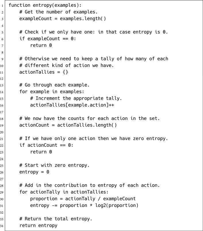
In this pseudo-code I have used the log2 function which gives the logarithm to base 2. As we saw earlier, this can be implemented as:

Although this is strictly correct, it isn’t necessary. We aren’t interested in finding the exact information gain. We are only interested in finding the greatest information gain. Because logarithms to any positive power retain the same order (i.e., if log₂ x > log₂ y then log_e x > log_e y), we can simply use the basic log in place of log₂, and save on the floating point division.

The actionTallies variable acts both as a dictionary indexed by the action (we increment its values) and as a list (we iterate through its values). This can be implemented as a basic hash map, although care needs to be taken to initialize a previously unused entry to zero before trying to increment it.

Entropy of Sets

Finally, we can implement the function to find the entropy of a list of lists:

Data Structures and Interfaces

In addition to the unusual data structures used to accumulate subsets and keep a count of actions in the functions above, the algorithm only uses simple lists of examples. These do not change size after they have been created, so they can be implemented as arrays. Additional sets are created as the examples are divided into smaller groups. In C or C++, it is sensible to have the arrays refer by pointer to a single set of examples, rather than copying example data around constantly.

The pseudo-code assumes that examples have the following interface:

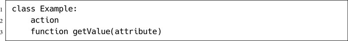
where getValue returns the value of a given attribute.

The ID3 algorithm does not depend on the number of attributes. action, not surprisingly, holds the action that should be taken given the attribute values.

Starting the Algorithm

The algorithm begins with a set of examples. Before we can call makeTree, we need to get a list of attributes and an initial decision tree node. The list of attributes is usually consistent over all examples and fixed in advance (i.e., we’ll know the attributes we’ll be choosing from); otherwise, we may need an additional application-dependent algorithm to work out the attributes that are used.

The initial decision node can simply be created empty. So the call may look something like:

Performance

The algorithm is O(a log_v n) in memory and O(avn log_v n) in time, where a is the number of attributes, v is the number of values for each attribute, and n is the number of examples in the initial set.

7.6.2  ID3 WITH CONTINUOUS ATTRIBUTES

ID3-based algorithms cannot operate directly with continuous attributes, and they are impractical when there are many possible values for each attribute. In either case the attribute values must be divided into a small number of discrete categories (usually two). This division can be performed automatically as an independent process, and with the categories in place the rest of the decision tree learning algorithm remains identical.

Single Splits

Continuous attributes can be used as the basis of binary decisions by selecting a threshold level. Values below the level are in one category, and values above the level are in another category. A continuous health value, for example, can be split into healthy and hurt categories with a single threshold value.

We can dynamically calculate the best threshold value to use with a process similar to that used to determine which attribute to use in a branch.

We sort the examples using the attribute we are interested in. We place the first element from the ordered list into category A and the remaining elements into category B. We now have a division, so we can perform the split and calculate information gained, as before.

We repeat the process by moving the lowest valued example from category B into category A and calculating the information gained in the same way. Whichever division gave the greatest information gained is used as the division. To enable future examples not in the set to be correctly classified by the resulting tree, we need a numeric threshold value. This is calculated by finding the average of the highest value in category A and the lowest value in category B.

This process works by trying every possible position to place the threshold that will give different daughter sets of examples. It finds the split with the best information gain and uses that.

The final step constructs a threshold value that would have correctly divided the examples into its daughter sets. This value is required, because when the decision tree is used to make decisions, we aren’t guaranteed to get the same values as we had in our examples: the threshold is used to place all possible values into a category.

As an example, consider a situation similar to that in the previous section. We have a health attribute, which can take any value between 0 and 200. We will ignore other observations and consider a set of examples with just this attribute.

50	Defend
25	Defend
39	Attack
17	Defend

We start by ordering the examples, placing them into the two categories, and calculating the information gained.

Category	Attribute Value	Action	Information Gain
A	17	Defend
B	25	Defend
	39	Attack
	50	Defend	0.12
Category	Attribute Value	Action	Information Gain
A	17	Defend
	25	Defend
B	39	Attack
	50	Defend	0.31
Category	Attribute Value	Action	Information Gain
A	17	Defend
	25	Defend
	39	Attack
B	50	Defend	0.12

We can see that the most information is gained if we put the threshold between 25 and 39. The midpoint between these values is 32, so 32 becomes our threshold value. Notice that the threshold value depends on the examples in the set. Because the set of examples gets smaller at each branch in the tree, we can get different threshold values at different places in the tree. This means that there is no set dividing line. It depends on the context. As more examples are available, the threshold value can be fine-tuned and made more accurate.

Determining where to split a continuous attribute can be incorporated into the entropy checks for determining which attribute to split on. In this form our algorithm is very similar to the C4.5 decision tree algorithm.

Pseudo-Code

We can incorporate this threshold step in the splitByAttribute function from the previous pseudo-code.

The sortReversed function takes a list of examples and returns a list of examples in order of decreasing value for the given attribute.

In the framework I described previously for makeTree, there was no facility for using a threshold value (it wasn’t appropriate if every different attribute value was sent to a different branch). In this case we would need to extend makeTree so that it receives the calculated threshold value and creates a decision node for the tree that could use it. In Chapter 5, Section 5.2 I described a FloatDecision class that would be suitable.

Data Structures and Interfaces

In the code above the list of examples is held in a stack. An object is removed from one list and added to another list using push and pop. Many collection data structures have these fundamental operations. If you are implementing your own lists, using a linked list, for example, this can be simply achieved by moving the “next“ pointer from one list to another.

Performance

The attribute splitting algorithm is O(n) in both memory and time, where n is the number of examples. Note that this is O(n) per attribute. If you are using it within ID3, it will be called once for each attribute.

Implementation Notes

In this section I have described a decision tree using either binary decisions (or at least those with a small number of branches) or threshold decisions.

In a real game, you are likely to need a combination of both binary decisions and threshold decisions in the final tree. The makeTree algorithm needs to detect what type best suits each algorithm and to call the correct version of splitByAttribute. The result can then be compiled into either a MultiDecision node or a FloatDecision node (or some other kind of decision nodes, if they are suitable, such as an integer threshold). This selection depends on the attributes you will be working with in your game.

Multiple Categories

Not every continuous value is best split into two categories based on a single threshold value. For some attributes there are more than two clear regions that require different decisions. A character who is only hurt, for example, will behave differently from one who is almost dead.

A similar approach can be used to create more than one threshold value. As the number of splits increases, there is an exponential increase in the number of different scenarios that must have their information gains calculated.

There are several algorithms for multi-splitting input data for lowest entropy. In general, the same thing can also be achieved using any classification algorithm, such as a neural network.

In game applications, however, multi-splits are seldom necessary. As the ID3 algorithm recurses through the tree, it can create several branching nodes based on the same attribute value. Because these splits will have different example sets, the thresholds will be placed at different locations. This allows the algorithm to effectively divide the attribute into more than two categories over two or more branch nodes. The extra branches will slow down the final decision tree a little, but since running a decision tree is a very fast process, this will not generally be noticeable.

Figure 7.11: Two sequential decisions on the same attribute

Figure 7.11 shows the decision tree created when the example data above is run through two steps of the algorithm. Notice that the second branch is subdivided, splitting the original attribute into three sections.

7.6.3  INCREMENTAL DECISION TREE LEARNING

So far I have described learning decision trees as a single task. A complete set of examples is provided, and the algorithm returns a complete decision tree ready for use. This is fine for offline learning, where a large number of observation–action examples can be provided in one go. The learning algorithm can spend a short time processing the example set to generate a decision tree.

When used online, however, new examples will be generated while the game is running, and the decision tree should change over time to accommodate them. With a small number of examples, only broad brush sweeps can be seen, and the tree will typically need to be quite flat. With hundreds or thousands of examples, subtle interactions between attributes and actions can be detected by the algorithm, and the tree is likely to be more complex.

The simplest way to support this scaling is to re-run the algorithm each time a new example is provided. This guarantees that the decision tree will be the best possible at each moment. Unfortunately, we have seen that decision tree learning is a moderately inefficient process. With large databases of examples, this can prove very time consuming.

Incremental algorithms update the decision tree based on the new information, without requiring the whole tree to be rebuilt.

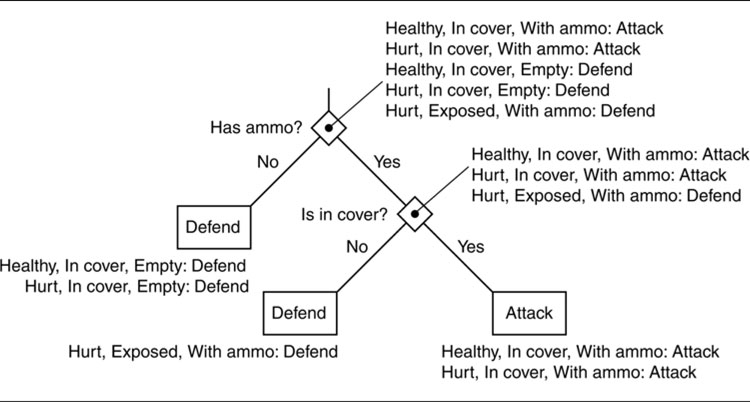
Figure 7.12: The example tree in ID4 format

The simplest approach would be to take the new example and use its observations to walk through the decision tree. When we reach a terminal node of the tree, we compare the action there with the action in our example. If they match, then no update is required, and the new example can simply be added to the example set at that node. If the actions do not match, then the node is converted into a decision node using SPLIT_NODE in the normal way.

This approach is fine, as far as it goes, but it always adds further examples to the end of a tree and can generate huge trees with many sequential branches. We ideally would like to create trees that are as flat as possible, where the action to carry out can be determined as quickly as possible.

The Algorithm

The simplest useful incremental algorithm is ID4. As its name suggests, it is related to the basic ID3 algorithm.

We start with a decision tree, as created by the basic ID3 algorithm. Each node in the decision tree also keeps a record of all the examples that reach that node. Examples that would have passed down a different branch of the tree are stored elsewhere in the tree. Figure 7.12 shows the ID4-ready tree for the example introduced earlier.

In ID4 we are effectively combining the decision tree with the decision tree learning algorithm. To support incremental learning, we can ask any node in the tree to update itself given a new example.

When asked to update itself, one of three things can happen:

1.  If the node is a terminal node (i.e., it represents an action), and if the added example also shares the same action, then the example is added to the list of examples for that node.

2.  If the node is a terminal node, but the example’s action does not match, then we make the node into a decision and use the ID3 algorithm to determine the best split to make.

3.  If the node is not a terminal node, then it is already a decision. We determine the best attribute to make the decision on, adding the new example to the current list. The best attribute is determined using the information gain metric, as we saw in ID3.

•  If the attribute returned is the same as the current attribute for the decision (and it will be most times), then we determine which of the daughter nodes the new example gets mapped to, and we update that daughter node with the new example.

•  If the attribute returned is different, then it means the new example makes a different decision optimal. If we change the decision at this point, then all of the tree further down the current branch will be invalid. So we delete the whole tree from the current decision down and perform the basic ID3 algorithm using the current decision’s examples plus the new one.

Note that when we reconsider which attribute to make a decision on, several attributes may provide the same information gain. If one of them is the attribute we are currently using in the decision, then we favor that one to avoid unnecessary rebuilding of the decision tree.

In summary, at each node in the tree, ID4 checks if the decision still provides the best information gain in light of the new example. If it does, then the new example is passed down to the appropriate daughter node. If it does not, then the whole tree is recalculated from that point on. This ensures that the tree remains as flat as possible.

In fact, the tree generated by ID4 will always be the same as that generated by ID3 for the same input examples. At worst, ID4 will have to do the same work as ID3 to update the tree. At best, it is as efficient as the simple update procedure. In practice, for sensible sets of examples, ID4 is considerably faster than repeatedly calling ID3 each time and will be faster in the long run than the simple update procedure (because it is producing flatter trees).

Walk Through

It is difficult to visualize how ID4 works from the algorithm description alone, so let’s work through an example.

We have seven examples. The first five are similar to those used before:

Healthy	Exposed	Empty	Run
Healthy	In Cover	With Ammo	Attack
Hurt	In Cover	With Ammo	Attack
Healthy	In Cover	Empty	Defend
Hurt	In Cover	Empty	Defend

Figure 7.13: Decision tree before ID4

We use these to create our initial decision tree. The decision tree looks like that shown in Figure 7.13.

We now add two new examples, one at a time, using ID4:

Hurt	Exposed	With Ammo	Defend
Healthy	Exposed	With Ammo	Run

The first example enters at the first decision node. ID4 uses the new example, along with the five existing examples, to determine that ammo is the best attribute to use for the decision. This matches the current decision, so the example is sent to the appropriate daughter node.

Currently, the daughter node is an action: attack. The action doesn’t match, so we need to create a new decision here. Using the basic ID3 algorithm, we decide to make the decision based on cover. Each of the daughters of this new decision have only one example and are therefore action nodes.

The current decision tree is then as shown in Figure 7.14.

Now we add our second example, again entering at the root node. ID4 determines that this time ammo can’t be used, so cover is the best attribute to use in this decision.

So we throw away the sub-tree from this point down (which is the whole tree, since we’re at the first decision) and run an ID3 algorithm with all the examples. The ID3 algorithm runs in the normal way and leaves the tree complete. It is shown in Figure 7.15.

Problems with ID4

ID4 and similar algorithms can be very effective in creating optimal decision trees. As the first few examples come in, the tree will be largely rebuilt at each step. As the database of examples grows, the changes to the tree often decrease in size, keeping the execution speed high.

Figure 7.14: Decision tree during ID4

Figure 7.15: Decision tree after ID4

It is possible, however, to have sets of examples for which the order of attribute tests in the tree is pathological: the tree continues to be rebuilt at almost every step. This can end up being slower than simply running ID3 each step. ID4 is sometimes said to be incapable of learning certain concepts. This doesn’t mean that it generates invalid trees (it generates the same trees as ID3), it just means that the tree isn’t stable as new examples are provided.

In practice, I haven’t suffered from this problem with ID4. Real data do tend to stabilize quite rapidly, and ID4 ends up significantly faster than rebuilding the tree with ID3 each time.

Other incremental learning algorithms, such as ID5, ITI, and their relatives, all use this kind of transposition, statistical records at each decision node, or additional tree restructuring operations to help avoid repeated rebuilding of the tree.

Heuristic Algorithms

Strictly speaking, ID3 is a heuristic algorithm: the information gain value is a good estimate of the utility of the branch in the decision tree, but it may not be the best. Other methods have been used to determine which attributes to use in a branch. One of the most common, the gain-ratio, was suggested by Quinlan, the original inventor of ID3.

Often, the mathematics is significantly more complex than that in ID3, and, while improvements have been made, the results are often highly domain-specific. Because the cost of running a decision tree in game AI is so small, it is rarely worth the additional effort. We know of few developers who have invested in developing anything more than simple optimizations of the ID3 scheme.

More significant speed ups can be achieved in incremental update algorithms when doing online learning. Heuristics can also be used to improve the speed and efficiency of incremental algorithms. This approach is used in algorithms such as SITI and other more exotic versions of decision tree learning.

7.7  REINFORCEMENT LEARNING

Reinforcement learning is the name given to a range of techniques for learning based on experience. In its most general form a reinforcement learning algorithm has three components: an exploration strategy for trying out different actions in the game, a reinforcement function that gives feedback on how good each action is, and a learning rule that links the two together. Each element has several different implementations and optimizations, depending on the application.

Later in this section we’ll look briefly at a range of reinforcement learning techniques. It is possible to do reinforcement learning with neural networks, both shallow and deep. In game applications, however, a good starting point is the Q-learning algorithm. Q-learning is simple to implement, has been widely tested on non-game applications, and can be tuned without a deep understanding of its theoretical properties.

7.7.1  THE PROBLEM

We would like a game character to select better actions over time. What makes a good action may be difficult to anticipate by the designers. It may depend on the way the player acts, or it may depend on the structure of random maps that can’t be designed for.

We would like to be able to give a character free choice of any action in any circumstance and for it to work out which actions are best for any given situation.

Unfortunately, the quality of an action isn’t normally clear at the time the action is made. It is relatively easy to write an algorithm that gives good feedback when the character collects a power-up or kills an enemy. But the actual killing action may have been only 1 out of 100 actions that led to the result, each one of which needed to be correctly placed in series.

Therefore, we would like to be able to give very patchy information: to be able to give feedback only when something significant happens. The character should learn that all the actions leading up to the event are also good things to do, even though no feedback was given while it was doing them.

7.7.2  THE ALGORITHM

Q-learning relies on having the problem represented in a particular way. With this representation in place, it can store and update relevant information as it explores the possible actions it can take. I will describe the representation first.

Q-Learning’s Representation of the World

Q-learning treats the game world as a state machine. At any point in time, the algorithm is in some state. The state should encode all the relevant details about the character’s environment and internal data.

So if the health of the character is significant to learning, and if the character finds itself in two identical situations with two different health levels, then it will consider them to be different states. Anything not included in the state cannot be learned. If we didn’t include the health value as part of the state, then we couldn’t possibly learn to take health into consideration in the decision making.

In a game the states are made up of many factors: position, proximity of the enemy, health level, and so on. Q-learning doesn’t need to understand the components of a state. As far as the algorithm is concerned they can just be an integer value: the state number.

The game, on the other hand, needs to be able to translate the current state of the game into a single state number for the learning algorithm to use. Fortunately, the algorithm never requires the opposite: we don’t have to translate the state number back into game terms (as we did in the pathfinding algorithm, for example).

Q-learning is known as a model-free algorithm because it doesn’t try to build a model of how the world works. It simply treats everything as states. Algorithms that are not model free try to reconstruct what is happening in the game from the states that it visits. Model-free algorithms, such as Q-learning, tend to be significantly easier to implement.

For each state, the algorithm needs to understand the actions that are available to it. In many games all actions are available at all times. For more complex environments, however, some actions may only be available when the character is in a particular place (e.g., pulling a lever), when they have a particular object (e.g., unlocking a door with a key), or when other actions have been properly carried out before (e.g., walking through the unlocked door).

After the character carries out one action in the current state, the reinforcement function should give it feedback. Feedback can be positive or negative and is often zero if there is no clear indication as to how good the action was. Although there are no limits on the values that the function can return, it is common to assume they will be in the range [−1, 1].

There is no requirement for the reinforcement value to be the same every time an action is carried out in a particular state. There may be other contextual information not used to create the algorithm’s state. As we saw previously, the algorithm cannot learn to take advantage of that context if it isn’t part of its state, but it will tolerate its effects and learn about the overall success of an action, rather than its success on just one attempt.

After carrying out an action, the character is likely to enter a new state. Carrying out the same action in exactly the same state may not always lead to the same state of the game. Other characters and the player are also influencing the state of the game.

For example, a character in an FPS is trying to find a health pack and avoid getting into a fight. The character is ducking behind a pillar. On the other side of the room, an enemy character is standing in the doorway looking around. So the current state of the character may correspond to in-room1, hidden, enemy-near, near-death. It chose the “hide” action to continue ducking. The enemy stays put, so the “hide” action leads back to the same state. So it chooses the same action again. This time the enemy leaves, so the “hide” action now leads to another state, corresponding to in-room1, hidden, no-enemy, near-death.

One of the powerful features of the Q-learning algorithm (and most other reinforcement algorithms) is that it can cope with this kind of uncertainty.

These four elements—the start state, the action taken, the reinforcement value, and the resulting state—are called the experience tuple, often written as < s, a, r, s′ >.

Doing Learning

Q-learning is named for the set of quality information (Q-values) it holds about each possible state and action. The algorithm keeps a value for every state and action it has tried. The Q-value represents how good it thinks that action is to take when in that state.

The experience tuple is split into two sections. The first two elements (the state and action) are used to look up a Q-value in the store. The second two elements (the reinforcement value and the new state) are used to update the Q-value based on how good the action was and how good it will be in the next state.

The update is handled by the Q-learning rule:

$Q\left(s,a\right)=\left(1-\alpha \right)Q\left(s,a\right)+\alpha \left(r+\gamma \max \left(Q\left(s^{\prime },a^{\prime }\right)\right)\right)$

where α is the learning rate and γ is the discount rate: both are parameters of the algorithm. The rule is sometimes written in a slightly different form, with the (1–α) multiplied out.

How It Works

The Q-learning rule blends together two components using the learning rate parameter to control the linear blend. The learning rate parameter, used to control the blend, is in the range [0, 1].

The first component Q(s, a) is simply the current Q-value for the state and action. Keeping part of the current value in this way means we never throw away information we have previously discovered.

The second component has two elements of its own. The r value is the new reinforcement from the experience tuple. If the reinforcement rule was

$Q\left(s,a\right)=\left(1-\alpha \right)Q\left(s,a\right)+\alpha r$

We would be blending the old Q-value with the new feedback on the action.

The second element, γ max(Q(s′ a′)), looks at the new state from the experience tuple. It looks at all possible actions that could be taken from that state and chooses the highest corresponding Q-value. This helps bring the success (i.e., the Q-value) of a later action back to earlier actions: if the next state is a good one, then this state should share some of its glory.

The discount parameter controls how much the Q-value of the current state and action depends on the Q-value of the state it leads to. A very high discount will be a large attraction to good states, and a very low discount will only give value to states that are near to success. Discount rates should be in the range [0, 1]. A value greater than 1 can lead to ever-growing Q-values, and the learning algorithm will never converge on the best solution.

So, in summary, the Q-value is a blend between its current value and a new value, which combines the reinforcement for the action and the quality of the state the action led to.

Exploration Strategy

So far we’ve covered the reinforcement function, the learning rule, and the internal structure of the algorithm. We know how to update the learning from experience tuples and how to generate those experience tuples from states and actions. Reinforcement learning systems also require an exploration strategy: a policy for selecting which actions to take in any given state. It is often simply called the policy.

The exploration strategy isn’t strictly part of the Q-learning algorithm. Although the strategy outlined below is very commonly used in Q-learning, there are others with their own strengths and weaknesses. In a game, a powerful alternative technique is to incorporate the actions of a player, generating experience tuples based on their play. We’ll return to this idea later in the section.

The basic Q-learning exploration strategy is partially random. Most of the time, the algorithm will select the action with the highest Q-value from the current state. The remainder, the algorithm will select a random action. The degree of randomness can be controlled by a parameter.

Convergence and Ending

If the problem always stays the same, and rewards are consistent (which they often aren’t if they rely on random events in the game), then the Q-values will eventually converge. Further running of the learning algorithm will not change any of the Q-values. At this point the algorithm has learned the problem completely.

For very small toy problems this is achievable in a few thousand iterations, but in real problems it can take a vast number of iterations. In a practical application of Q-learning, there won’t be nearly enough time to reach convergence, so the Q-values will be used before they have settled down. It is common to begin acting under the influence of the learned values before learning is complete.

7.7.3  PSEUDO-CODE

A general Q-learning system has the following structure:

I am assuming that the random function returns a floating point number between zero and one. The oneOf function picks an item from a list at random.

7.7.4  DATA STRUCTURES AND INTERFACES

The algorithm needs to understand the problem—what state it is in, what actions it can take—and after taking an action it needs to access the appropriate experience tuple. The code above does this through an interface of the following form:

In addition, the Q-values are stored in a data structure that is indexed by both state and action. This has the following form in our example:

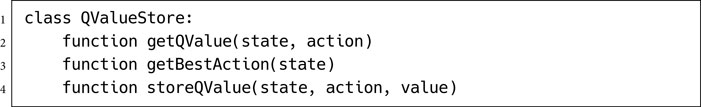
The getBestAction function returns the action with the highest Q-value for the given state. The highest Q-value (needed in the learning rule) can be found by calling getQValue with the result from getBestAction.

7.7.5  IMPLEMENTATION NOTES

If the Q-learning system is designed to operate online, then the Q-learning function should be rewritten so that it only performs one iteration at a time and keeps track of its current state and Q-values in a data structure.

The store can be implemented as a hash table indexed by an action–state pair. Only action–state pairs that have been stored with a value are contained in the data structure. All other indices have an implicit value of zero. So getQValue will return zero if the given action–state pair is not in the hash. This is a simple implementation that can be useful for doing brief bouts of learning. It suffers from the problem that getBestAction will not always return the best action. If all the visited actions from the given state have negative Q-values and not all actions have been visited, then it will pick the highest negative value, rather than the zero value from one of the non-visited actions in that state.

Q-learning is designed to run through all possible states and actions, probably several times (I will return to the practicality of this below). In this case, the hash table will be a waste of time (literally). A better solution is an array indexed by the state. Each element in this array is an array of Q-values, indexed by action. All the arrays are initialized to have zero Q-values. Q-values can now be looked up immediately, as they are all stored.

7.7.6  PERFORMANCE

The algorithm’s performance scales based on the number of states and actions, and the number of iterations of the algorithm. It is preferable to run the algorithm so that it visits all of the states and actions several times. In this case it is O(i) in time, where i is the number of iterations of learning. It is O(as) in memory, where a is the number of actions, and s is the number of states per action. We are assuming that arrays are used to store Q-values in this case.

If O(i) is very much less than O(as), then it might be more efficient to use a hash table; however, this has corresponding increases in the expected execution time.

7.7.7  TAILORING PARAMETERS

The algorithm has four parameters with the variable names alpha, gamma, rho, and nu in the pseudo-code above. The first two correspond to the α and γ parameters in the Q-learning rule. Each has a different effect on the outcome of the algorithm and is worth looking at in detail.

Alpha: The Learning Rate

The learning rate controls how much influence the current feedback value has over the stored Q-value. It is in the range [0, 1].

A value of zero would give an algorithm that does not learn: the Q-values stored are fixed and no new information can alter them. A value of one would give no credence to any previous experience. Any time an experience tuple is generated that alone is used to update the Q-value.

From my experimentation, I found that a value of 0.3 is a sensible initial guess, although tuning is needed. In general, a high degree of randomness in your state transitions (i.e., if the reward or end state reached by taking an action is dramatically different each time) requires a lower alpha value. On the other hand, the fewer iterations the algorithm will be allowed to perform, the higher the alpha value will be.

Learning rate parameters in many machine learning algorithms benefit from being changed over time. Initially, the learning rate parameter can be relatively high (0.7, say). Over time, the value can be gradually reduced until it reaches a lower than normal value (0.1, for example). This allows the learning to rapidly change Q-values when there is little information stored in them, but protects hard-won learning later on.

Gamma: The Discount Rate

The discount rate controls how much an action’s Q-value depends on the Q-value at the state (or states) it leads to. It is in the range [0, 1].

A value of zero would rate every action only in terms of the reward it directly provides. The algorithm would learn no long-term strategies involving a sequence of actions. A value of one would rate the reward for the current action as equally important as the quality of the state it leads to.

Higher values favor longer sequences of actions, but take correspondingly longer to learn. Lower values stabilize faster, but usually support relatively short sequences. It is possible to select the way rewards are provided to increase the sequence length (see the later section on reward values), but again this makes learning take longer.

A value of 0.75 is a good initial value to try, again based on my experimentation. With this value, an action with a reward of 1 will contribute 0.05 to the Q-value of an action ten steps earlier in the sequence.

Rho: Randomness for Exploration

This parameter controls how often the algorithm will take a random action, rather than the best action it knows so far. It is in the range [0, 1].

A value of zero would give a pure exploitation strategy: the algorithm would exploit its current learning, reinforcing what it already knows. A value of one would give a pure exploration strategy: the algorithm would always be trying new things, never benefiting from its existing knowledge.

This is a classic trade-off in learning algorithms: to what extent should we try to learn new things (which may be much worse than the things we know are good), and to what extent should we exploit the knowledge we have gained. The biggest factor in selecting a value is whether the learning is performed online or offline.

If learning is being performed online, then the player will want to see some kind of intelligent behavior. The learning algorithm should be exploiting its knowledge. If a value of one was used, then the algorithm would never use its learned knowledge and would always appear to be making decisions at random (it is doing so, in fact). Online learning demands a low value (0.1 or less should be fine).

For offline learning, however, we simply want to learn as much as possible. Although a higher value is preferred, there is still a trade-off to be made.

Often, if one state and action are excellent (have a high Q-value), then other similar states and actions will also be good. If we have learned a high Q-value for killing an enemy character, for example, we will probably have high Q-values for bringing the character close to death. So heading toward known high Q-values is often a good strategy for finding other action–state pairs with good Q-values.

It takes several iterations for a high Q-value to propagate back along the sequence of actions. To distribute Q-values so that there is a sequence of actions to follow, there needs to be several iterations of the algorithm in the same region.

Following actions known to be good helps both of these issues. A good starting point for this parameter, in offline learning, is 0.2. This value is once again my favorite initial guess from previous experience.

Nu: The Length of Walk

The length of walk controls the number of iterations that will be carried out in a sequence of connected actions. It is in the range [0, 1].

A value of zero would mean the algorithm always uses the state it reached in the previous iteration as the starting state for the next iteration. This has the benefit of the algorithm seeing through sequences of actions that might eventually lead to success. It has the disadvantage of allowing the algorithm to get caught in a relatively small number of states from which there is no escape or an escape only by a sequence of actions with low Q-values (which are therefore unlikely to be selected).

A value of one would mean that every iteration starts from a random state. If all states and all actions are equally likely, then this is the optimal strategy: it covers the widest possible range of states and actions in the smallest possible time. In reality, however, some states and actions are far more prevalent. Some states act as attractors, to which a large number of different action sequences lead. These states should be explored in preference to others, and allowing the algorithm to wander along sequences of actions accomplishes this.

Many exploration policies used in reinforcement learning do not have this parameter and assume that it has the value zero. They always wander in a connected sequence of actions. In online learning, the state used by the algorithm is directly controlled by the state of the game, so it is impossible to move to a new random state. In this case a value of zero is enforced.

Figure 7.16: A learned state machine

In my experimentation with reinforcement learning, especially in applications where only a limited number of iterations are possible, values of around 0.1 are suitable. This produces sequences of about nine actions in a row, on average.

Choosing Rewards

Reinforcement learning algorithms are very sensitive to the reward values used to guide them. It is important to take into account how the reward values will be used when you use the algorithm.

Typically, rewards are provided for two reasons: for reaching the goal and for performing some other beneficial action. Similarly, negative reinforcement values are given for “losing” the game (e.g., dying) or for taking some undesired action. This may seem a contrived distinction. After all, reaching the goal is just a (very) beneficial action, and a character should find its own death undesirable.

Much of the literature on reinforcement learning assumes that the problem has a solution and that reaching the goal state is a well-defined action. In games (and other applications) this isn’t the case. There may be many different solutions, of different qualities, and there may be no final solutions at all but instead hundreds or thousands of different actions that are beneficial or problematic.

In a reinforcement learning algorithm with a single solution, we can give a large reward (let’s say 1) to the action that leads to the solution and no reward to any other action. After enough iterations, there will be a trail of Q-values that leads to the solution. Figure 7.16 shows Q-values labeled on a small problem (represented as a state machine diagram). The Q-learning algorithm has been run a huge number of times, so the Q-values have converged and will not change with additional execution.

Starting at node A, we can simply follow the trail of increasing Q-values to get to the solution. In the language of search (described earlier), we are hill climbing. Far from the solution the Q-values are quite small, but this is not an issue because the largest of these values still points in the right direction.

Figure 7.17: A learned machine with additional rewards

If we add additional rewards, the situation may change. Figure 7.17 shows the results of another learning exercise.

If we start at state A, we will get to state B, whereupon we can get a small reward from the action that leads to C. At C, however, we are far enough from the solution that the best action to take is to go back to B and get the small reward again. Hill climbing in this situation leads us to a sub-optimal strategy: constantly taking the small reward rather than heading for the solution. The problem is said to be unimodal if there is only one hill and multi-modal if there are multiple hills. Hill climbing algorithms don’t do well on multi-modal problems, and Q-learning is no exception.

The situation is made worse with multiple solutions or lots of reward points. Although adding rewards can speed up learning (you can guide the learning toward the solution by rewarding it along the way), it often causes learning to fail completely. There is a fine balance to achieve. Using very small values for non-solution rewards helps, but cannot completely eliminate the problem.

As a rule of thumb, try to simplify the learning task so that there is only one solution and so you don’t give any non-solution rewards. Add in other solutions and small rewards only if the learning takes too long or gives poor results.

7.7.8  WEAKNESSES AND REALISTIC APPLICATIONS

Reinforcement learning has not been widely used in game development. It is one of a new batch of promising techniques often taught in undergraduate AI courses, that is receiving interest in the industry.

Like many of these new technologies, the practicality doesn’t match some of the potential. Game development websites and articles written by those outside the industry can appear effusive. It is worth taking a dispassionate look at their real applicability.

Limits of the Algorithm

Q-learning requires the game to be represented as a set of states linked by actions. The algorithm is very sensitive in its memory requirements to the number of states and actions. The state of a game is typically very complex. If the position of characters is represented as a three-dimensional (3D) vector, then there is an effectively infinite number of states. Clearly, we need to group sets of states together to send to the Q-learning algorithm.

Just like for pathfinding, we can divide up areas of the game level. We can also quantize health values, ammo levels, and other bits of state so that they can be represented with a handful of different discrete values. Similarly, we can represent flexible actions (such as movement in two dimensions) with discrete approximations.

The game state consists of a combination of all these elements, however, producing a huge problem. If there are 100 locations in the game and 20 characters, each with 4 possible health levels, 5 possible weapons, and 4 possible ammo levels, then there will be (100*4*4*5)¹⁰ states, roughly 10⁵⁰. Clearly, no algorithm that is O(as) in memory will be viable.

Even if we dramatically slash the number of states so that they can be fit in memory, we have an additional problem. The algorithm needs to run long enough so that it tries out each action at each state several times. In fact, the quality of the algorithm can only be proved in convergence: it will eventually end up learning the right thing. But eventually could entail many hundreds of visits to each state.

In reality, we can often get by with tweaking the learning rate parameter, using additional rewards to guide learning and applying dramatically fewer iterations.

After a bit of experimentation, I estimate that the technique is practically limited to around 1 million states, with 10 actions per state. We can run around 1 billion iterations of the algorithm to get workable (but not great) results, and this can be done in reasonable time scales (a few minutes) and with reasonable memory. Obviously, solving a problem once offline with more beefy machines could increase the size somewhat, particularly if the algorithm is implemented to run on the graphics card, but it will still only buy an extra order of magnitude or two.

Online learning should probably be limited to problems with less than 1000 states, given that the rate that states can be explored is so limited.

Applications

Reinforcement learning is most suitable for offline learning. It works well for problems with lots of different interacting components, such as optimizing the behavior of a group of characters or finding sequences of order-dependent actions. Its main strength is its ability to seamlessly handle uncertainty. This allows us to simplify the states exposed to it; we don’t have to tell the algorithm everything.

It is not suitable for problems where there is an easy way to see how close a solution is (we can use some kind of planning here), where there are too many states, or where the strategies that are successful change over time (i.e., it requires a good degree of stability to work).

It can be applied to choosing tactics based on knowledge of enemy actions (see below), for bootstrapping a whole character AI for a simple character (we simply give it a goal and a range of actions), for limited control over character or vehicle movement, for learning how to interact socially in multi-player games, for determining how and when to apply one specific behavior (such as learning to jump accurately or learning to fire a weapon), and for many other real-time applications.

It has proven particularly strong in board game AI, evaluating the benefit of a board position. By extension, it has a strong role to play in strategy setting in turn-based games and other slow moving strategic titles.

It can be used to learn the way a player plays and to mimic the player’s style, making it one choice for implementing a dynamic demo mode.

An Example Case Study: Choosing Tactical Defense Locations

Suppose we have a level in which a sentry team of three characters is defending the entrance to a military facility. There are a range of defensive locations that the team can occupy (15 in all). Each character can move to any empty location at will, although we will try to avoid everyone moving at the same time. We would like to determine the best strategy for character movement to avoid the player getting to the entrance safely.

The state of the problem can be represented by the defensive location occupied by each character (or no location if it is in motion), whether each character is still alive, and a flag to say if any of the characters can see the player. We therefore have 17 possible positional states per character (15 + in motion + dead) and 2 sighting states (player is either visible or not). Thus, there are 34 states per player, for a total of 40,000 states overall.

At each state, if no character is in motion, then one may change location. In this case there are 56 possible actions, and there are no possible actions when any character is in motion.

A reward function is provided if the player dies (characters are assumed to shoot on sight). A negative reward is given if any character is killed or if the player makes it to the entrance. Notice we aren’t representing where the player is when seen. Although it matters a great deal where the player is, the negative reward when the player makes it through means the strategy should learn that a sighting close to the entrance is more risky.

The reinforcement learning algorithm can be run on this problem. The game models a simple player behavior (random routes to the entrance, for example) and creates states for the algorithm based on the current game situation.

With no graphics to render, a single run of the scenario can be performed quickly.

To implement this I would use the 0.3 alpha, 0.7 gamma, and 0.3 rho values suggested previously. Because the state is linked to an active game state, nu will be 0 (we can’t restart from a random state, and we’ll always restart from the same state and only when the player is dead or has reached the entrance).

7.7.9  OTHER IDEAS IN REINFORCEMENT LEARNING

Reinforcement learning is a big topic, and one that I couldn’t possibly exhaust here. Because there has been such minor use of reinforcement learning in games, it is difficult to say what the most significant variations will be.

Q-learning is a well-established standard in reinforcement learning and has been applied to a huge range of problems. The remainder of this section provides a quick overview of other algorithms and applications.

TD

Q-learning is one of a family of reinforcement learning techniques called Temporal Difference algorithms (TD for short). TD algorithms have learning rules that update their value based on the reinforcement signal and on previous experience at the same state.

The basic TD algorithm stores values on a per-state basis, rather than using action–state pairs. They can therefore be significantly lighter on memory use, if there are many actions per state.

Because we are not storing actions as well as states, the algorithm is more reliant on actions leading to a definite next state. Q-learning can handle a much greater degree of randomness in the transition between states than vanilla TD.

Aside from these features, TD is very similar to Q-learning. It has a very similar learning rule, has both alpha and beta parameters, and responds similarly to their adjustment.

Off-Policy and On-Policy Algorithms

Q-learning is an off-policy algorithm. The policy for selecting the action to take isn’t a core part of the algorithm. Alternative strategies can be used, and as long as they eventually visit all possible states the algorithm is still valid.

On-policy algorithms have their exploration strategy as part of their learning. If a different policy is used, the algorithm might not reach a reasonable solution. Original versions of TD had this property. Their policy (choose the action that is most likely to head to a state with a high value) is intrinsically linked to their operation.

TD in Board Game AI

A simplified version of TD was used in Samuel’s Checkers-playing program, one of the most famous programs in AI history. Although it omitted some of the later advances in reinforcement learning that make up a regular TD algorithm, it had the same approach.

Another modified version of the TD was used in the famous Backgammon-playing program devised by Gerry Tesauro. It succeeded in reaching international-level play and contributed insights to Backgammon theory used by expert players. Tesauro combined the reinforcement learning algorithm with a neural network.

Neural Networks for Storage

As we have seen, memory is a significant limiting factor for the size of reinforcement learning problems that can be tackled. It is possible to use a neural network to act as a storage medium for Q-values (or state values, called V, in the regular TD algorithm).

Neural networks (as we will see in the next section) also have the ability to generalize and find patterns in data. Previously, I mentioned that reinforcement learning cannot generalize from its experience: if it works out that shooting a guard in one situation is a good thing, it will not immediately assume that shooting a guard in another situation is good. Using neural networks can allow the reinforcement learning algorithm to perform this kind of generalization. If the neural network is told that shooting an enemy in several situations has a high Q-value, it is likely to generalize and assume that shooting an enemy in other situations is also a good thing to do.

On the downside, neural networks are unlikely to return the same Q-value that was given to them. The Q-value for a action–state pair will fluctuate over the course of learning, even when it is not being updated (particularly if it is not, in fact). The Q-learning algorithm is therefore not guaranteed to come to a sensible result. The neural network tends to make the problem more multi-modal. As we saw in the previous section, multi-modal problems tend to produce sub-optimal character behavior.

So far I am not aware of any developers who have used this combination successfully, although its success in the TD Backgammon program suggests that its complexities can be tamed.

Actor–Critic

The actor–critic algorithm keeps two separate data structures: one of values used in the learning rule (Q-values, or V-values, depending on the flavor of learning) and another set that is used in the policy.

The eponymous actor is the exploration strategy; the policy that controls which actions are selected. This policy receives its own set of feedback from the critic, which is the usual learning algorithm. So as rewards are given to the algorithm, they are used to guide learning in the critic, which then passes on a signal (called a critique) to the actor, which uses it to guide a simpler form of learning.

The actor can be implemented in more than one way. There are strong candidates for policies that support criticism. The critic is usually implemented using the basic TD algorithm, although Q-learning is also suitable.

Actor–critic methods have been suggested for use in games by several developers. Their separation of learning and action theoretically provides greater control over decision making. In practice, I feel that the benefit is marginal at best. But I wait to be proved wrong by a developer with a particularly successful implementation.

7.8  ARTIFICIAL NEURAL NETWORKS

Artificial neural networks (ANNs, or just neural networks for short) were at the vanguard of the new “biologically inspired” computing techniques of the 1970s. Despite being used in a wide range of applications, their fame diminished until the mid-2010s when they exploded back to prominence as the main technique in deep learning.

Like many biologically inspired techniques, collectively called Natural Computing (NC), and before that other AI techniques, they have been the subject of a great deal of unreasonable hype. Since the successes of the 1960s, AI has always been on the verge of changing the world. Perhaps with deep learning that prospect will come true.

In games, neural networks attract a vocal following of pundits, particularly on websites and forums, who see their potential as a kind of panacea for the problems in AI.

Developers who have experimented with neural networks for large-scale behavior control tend to be more realistic about the approach’s weaknesses. The combined hype and disappointment have clouded the issue. AI-savvy hobbyists can’t understand why the industry isn’t using them more widely, and developers often see them as being useless and a dead end.

Personally, I’ve never used a neural network in a game. I have built neural network prototypes for a couple of AI projects, but none made it through to playable code. I can see, however, that they are a useful technique in the developer’s armory. In particular, I would strongly consider using them as a classification technique, which is their primary strength.

It will undeniably be an interesting ten years in neural-network-based AI. The reality of the games industry is that a strong success by one or two prominent studios can change the way people think about a technique. It is possible that deep learning will cross from its high-profile role in board games and game playing, to be a reliable technique for character design. Equally, it is possible that developers continue to work with simpler algorithms, feeling that they are sufficient, and easier to manage. When I wrote the first edition of this book, I didn’t expect the arrival of deep learning. And I can’t call what the state-of-the-art will be, when it comes to the fourth edition. For now I personally am keeping it in my toolbox.

In this section I can’t possibly hope to cover more than the basics of neural networks or deep learning.

Neural networks are a huge subject, full of different kinds of network and learning algorithms specialized for very small sets of tasks. Very little neural network theory is applicable to games, however. So I’ll stick to the basic technique with the widest usefulness. When it comes to deep learning, in this chapter I will gave an overview of the field, but focus on deep neural networks. I will talk about the application of deep learning to board games in Chapter 9. Deep learning builds on the basic algorithms of neural networks, so I will discuss neural networks in their simplest terms in the section, and return to deep learning in the next.

Neural Network Zoology

There is a bewildering array of different neural networks. They have evolved for specialized use, giving a branching family tree of intimidating depth. Practically everything we can think of to say about neural networks has exceptions. There are few things you can say about a neural network that is true of all of them.

So I am going to steer a sensible course. I will focus on a particular neural network in more detail: the multi-layer perceptron. And I will describe one particular learning rule: the backpropagation algorithm (backprop for short). Other techniques will be mentioned in passing.

It is an open question as to whether multi-player perceptrons are the most suited to game applications. They are the most common form of ANN, however. Until developers find an application that is obviously a “killer app” for neural networks in games, I think it is probably best to start with the most widespread technique.

7.8.1  OVERVIEW

Neural networks consist of a large number of relatively simple nodes, each running the same algorithm. These nodes are the artificial neurons, originally intended to simulate the operation of a single brain cell. Each neuron communicates with a subset of the other artificial neurons in the network. They are connected in patterns characteristic of the neural network type. This pattern is the neural network’s architecture or topology.

Architecture

Figure 7.18 shows a typical architecture for a multi-layer perceptron (MLP) network. Perceptrons (the specific type of artificial neuron used) are arranged in layers, where each perceptron is connected to all those in the layers immediately in front of and behind it.

The architecture on the right shows a different type of neural network: a Hopfield network. Here the neurons are arranged in a grid, and connections are made between neighboring points in the grid.

Feedforward and Recurrence

In many types of neural networks, some connections are specifically inputs and the others are outputs. The multi-layer perceptron takes inputs from all the nodes in the preceding layer and sends its single output value to all the nodes in the next layer. It is known as a feedforward network for this reason. The leftmost layer (called the input layer) is provided input by the programmer, and the output from the rightmost layer (called the output layer) is the output finally used to do something useful.

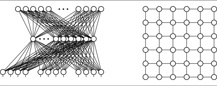
Figure 17.18: ANN architectures (MLP and Hopfield)

Feedforward networks can have loops: connections that lead from a later layer back to earlier layers. This architecture is known as a recurrent network. Recurrent networks can have very complex and unstable behavior and are typically much more difficult to control.

Other neural networks have no specific input and output. Each connection is both input and output at the same time.

Neuron Algorithm

As well as architecture, neural networks specify an algorithm. At any time the neuron has some state; you can think of it as an output value from the neuron (it is normally represented as a floating point number).

The algorithm controls how a neuron should generate its state based on its inputs. In a multi-layer perceptron network, the state is passed as an output to the next layer. In networks without specific inputs and outputs, the algorithm generates a state based on the states of connected neurons.

The algorithm is run by each neuron in parallel. For game machines that don’t have parallel capabilities (at least not of the right kind), the parallelism is simulated by getting each neuron to carry out the algorithm in turn. It is possible, but not common, to make different neurons have completely different algorithms.

We can treat each neuron as an individual entity running its algorithm. The perceptron algorithm is shown figuratively in Figure 7.19.

Each input has an associated weight. The input values (we’re assuming that they’re zero or one here) are multiplied by the corresponding weight. An additional bias weight is added (it is equivalent to another input whose input value is always one). The final sum is then passed through a threshold function. If the sum is less than zero, then the neuron will be off (have a value of zero); otherwise, it will be on (have a value of one).

Figure 7.19: Perceptron algorithm

The threshold function turns an input weight sum into an output value. We’ve used a hard step function (i.e., it jumps right from output = 0 to output = 1), but there are a large number of different functions in use. In order to make learning possible, the multi-layer perceptron algorithm uses slightly smoother functions, where values close to the step get mapped to intermediate output values. We’ll return to this in the next section.

Learning Rule

So far we haven’t talked about learning. Neural networks differ in the way they implement learning. For some networks learning is so closely entwined with the neuron algorithm that they can’t be separated. In most cases, however, the two are quite separate.

Multi-layer perceptrons can operate in two modes. The normal perceptron algorithm, described in the previous section, is used to put the network to use. The network is provided with input in its input layer; each of the neurons does its stuff, and then the output is read from the output layer. This is typically a very fast process and involves no learning. The same input will always give the same output (this isn’t the case for recurrent networks, but we’ll ignore these for now).

To learn, the multi-layer perceptron network is put in a specific learning mode. The task of the learning algorithm is to discover which weights are contributing to the correct answer, and which weights are not. The correct weights can then be reinforced (or possibly left as they are), and the incorrect weights can be changed. Unfortunately, for some input to the network, we are comparing desired outputs to actual outputs. Deciding which weights were important in generating the output is difficult. This is known as the credit assignment problem. The more intermediate layer a network has, more tricky it is to work out where any error has occurred.

There are various learning rules for the multi-layer perceptron. But the credit assignment problem is so complex that there is no one best rule for all situations. Here I will describe ‘backpropagation’, the most common, and the basis of many variations.

Where the network normally feeds forward, with each layer generating its output from the previous layer, backpropagation works in the opposite direction, working backward from the output.

At the end of this section, I will also describe1 Hebbian learning, a completely different learning rule that may be useful in games. For now, let us stick with backpropagation and work through the multi-layer perceptron algorithm.

7.8.2  THE PROBLEM

We’d like to group a set of input values (such as distances to enemies, health values for friendly units, or ammo levels) together so that we can act differently for each group. For example, we might have a group of “safe” situations, where health and ammo are high and enemies are a long way off. Our AI can go looking for power-ups or lay a trap in this situation. Another group might represent life-threatening situations where ammo is spent, health is perilously low, and enemies are bearing down. This might be a good time to run away in blind panic. So far, this is simple (and a decision tree would suffice). But say we also wanted a “fight-valiantly” group. If the character was healthy, with ammo and enemies nearby, it would naturally do its stuff. But it might do the same if it was on the verge of death, but had ammo, and it might do the same even in improbable odds to altruistically allow a squad member to escape. It may be a last stand, but the results are the same.

As these situations become more complex, and the interactions get more involved, it can become difficult to create the rules for a decision tree or fuzzy state machine.

We would like a method that learns from example (just like decision tree learning), allowing us to give a few tens of examples. The algorithm should generalize from examples to cover all eventualities. It should also allow us to add new examples during the game so that we can learn from mistakes.

What about Decision Tree Learning?

We could use decision tree learning to solve this problem: the output values correspond to the leaves of the decision tree, and the input values are used in the decision tree tests. If we used an incremental algorithm (such as ID4), we would also be able to learn from our mistakes during the game. For classification problems like this, decision tree learning and neural networks are viable alternatives.

Decision trees are accurate. They give a tree that correctly classifies from the given examples. To do this, they make hard and fast decisions. When they see a situation that wasn’t represented in their examples, they will make a decision based on it. Because their decision making is so hard and fast, they aren’t so good at generalizing by extrapolating into gray areas beyond the examples. Neural networks are not so accurate. They may even give the wrong responses for the examples provided. They are better, however, at extrapolating (sometimes sensibly) into those gray areas.

This trade-off between accuracy and generalization is the basis of the decision you must make when considering which technique to use. In my work, I’ve come down on the side of accuracy, but every application has its own peculiarities.

7.8.3  THE ALGORITHM

As an example for the algorithm, I will use a variation of the tactical situation we looked at previously. An AI-controlled character makes use of 19 input values: the distance to the nearest 5 enemies, the distance to the nearest 4 friends along with their health and ammo values, and the health and ammo of the AI. I will assume that there are five different output behaviors: run-away, fight-valiantly, heal-friend, hunt-enemy, and find-power-up. Assume that we have an initial set of 20 to 100 scenarios, each one a set of inputs with the output we’d like to see.

For now, we will use a network with three layers: input layer and output layer, as previously discussed, plus an intermediate (hidden) layer. This would qualify as a ‘shallow learning’ neural network, but as we will see in the next section, it is likely to be the best approach for this task.

The input layer has the same number of nodes as there are values in our problem: 19. The output layer has the same number of nodes as there are possible outputs: 5. Hidden layers are typically at least as large as the input layer and often much larger. The structure is shown in Figure 7.20, with some of the nodes omitted for clarity.

Each perceptron has a set of weights for each of the neurons in the previous layer. It also holds a bias weight. Input layer neurons do not have any weights. Their value is simply set by the corresponding values in the game.

We split our scenarios into two groups: a training set (used to do the learning) and a testing set (used to check on how learning is going). Ten training and ten testing examples would be an absolute minimum for this problem. Fifty of each would be much better.

Initial Setup and Framework

We start by initializing all the weights in the network to small random values.

We perform a number of iterations of the learning algorithm (typically hundreds or thousands). For each iteration we select an example scenario from the training set. Usually, the examples are chosen in turn, looping back to the first example after all of them have been used.

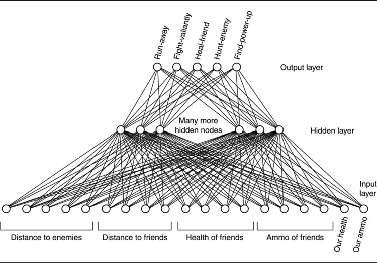
Figure 7.20: Multi-layer perceptron architecture

At each iteration we perform two steps. Feedforward takes the inputs and guesses an output, and backpropagation modifies the network based on the real output and the guess.

After the iterations are complete, and the network has learned, we can test if the learning was successful. We do this by running the feedforward process on the test set of examples. If the guessed output matches the output we were looking for, then it is a good sign that the neural network has learned properly. If it hasn’t, then we can run some more algorithms.

If the network continually gets the test set wrong, then it is an indication that there aren’t enough examples in the training set or that they aren’t similar enough to the test examples. We should give it more varied training examples.

Feedforward

First, we need to generate an output from the input values in the normal feedforward manner. We set the states of the input layer neurons directly. Then for each neuron in the hidden layer, we get it to perform its neuron algorithm: summing the weighted inputs, applying a threshold function, and generating its output. We can then do the same thing for each of the output layer neurons.

We need to use a slightly different threshold function from that described in the introduction. It is called the ReLU function (short for ‘rectified linear unit’), and it is shown in Figure 7.21. For input values below zero, it returns zero just like the step function. For input values greater than zero, the activation increases linearly. This will become important when it comes to learning, because we can differentiate neurons that very strongly fire from those that are more ambivalent about their decision.

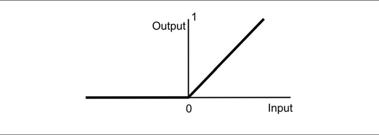
Figure 7.21: The ReLU function

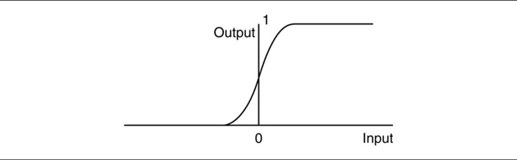
Figure 7.22: The sigmoid threshold function

This will be the function we will use for learning. Its equation is:

$f\left(x\right)=\max \left(0,x\right)$

or, in some cases a slightly smoother version (sometimes known as ‘softplus’, but often simply referred to as ReLU, as with the version that uses max):

$f\left(x\right)=\log \left(1+e^x\right)$

ReLU was introduced in 2011 [16], replacing a decades-old alternative called the ‘sigmoid function’. ReLU made a dramatic difference in the ability of large neural networks to learn efficiently. The sigmoid function can still be used on smaller networks, but as the number of intermediate layers increases, and the shallow network becomes deep, ReLU comes to dominate.

The main limitation of ReLU is that it is unbounded. Unlike the step function, there is no upper limit to how much activation a neuron can produce. In some cases this can lead to a network becoming saturated and it’s learning becoming stuck. In those cases an alternative may be needed.

Although it is now less often used, Figure 7.22 shows the sigmoid function. For input values far from zero, it acts just like the step function. For input values near to zero, it is smoother, giving us intermediate output. The equation of the function is:

$f\left(x\right)=\frac{1}{1+e^{-hx}}$

where h is a tweakable parameter that controls the shape of the function. The larger the value of h, the nearer to the step function this becomes. The best value of h depends on the number of neurons per layer and the size of the weights in the network. Both factors tend to lower the h value. The difficulty of optimizing the h value, and the sensitivity of learning to getting it right, is another reason to prefer ReLU. Because it is relatively new, much of the neural network literature still assumes a sigmoid function, so it is worth being aware of, but from here on we will stick to ReLU.

Backpropagation

To learn, we compare the state of the output nodes with the current pattern. The desired output is zero for all output nodes, except the one corresponding to our desired action. We work backward, a layer at a time, from the output layer, updating all the weights.

Let the set of neuron states be o_j, where j is the neuron, and w_ij is the weight between neurons i and j. The equation for the updated weight value is

${{\omega }^{\prime }}_{ij}={\omega }_{ij}+\eta {\delta }_j{o}_i$

where η is a gain term, and δ_j is an error term (both of which I’ll discuss below).

The equation says that we calculate the error in the current output for a neuron, and we update its weights based on which neurons affected it. So if a neuron comes up with a bad result (i.e., we have a negative error term), we go back and look at all its inputs. For those inputs that contributed to the bad output, we tone down the weights. On the other hand, if the result was very good (positive error term), we go back and strengthen weights from neurons that helped it. If the error term is somewhere in the middle (around zero), we make very little change to the weight.

The Error Term

The error term,δ_j, is calculated slightly differently depending on whether we are considering an output node (for which our pattern gives the output we want) and hidden nodes (where we have to deduce the error).

For the output nodes, the error term is given by:

${\delta }_j=o_j\left(1-o_j\right)\left(t_j-o_j\right)$

where t_j is the target output for node j. For hidden nodes, the error term relates the errors at the next layer up:

${\delta }_j=o_j\left(1-o_j\right){\displaystyle \sum _k{w}_{jk}{\delta }_k}$

where k is the set of nodes in the next layer up. This formula says that the error for a neuron is equal to the total error it contributes to the next layer. The error contributed to another node is w_kjδ_k, the weight of that node multiplied by the error of that node.

For example, let’s say that neuron A is on. It contributes strongly to neuron B, which is also on. We find that neuron B has a high error, so neuron A has to take responsibility for influencing B to make that error. The weight between A and B is therefore weakened.

The Gain

The gain term, η, controls how fast learning progresses. If it is close to zero, then the new weight will be very similar to the old weight. If weights are changing slowly, then learning is correspondingly slow. If η is a larger value (it is rarely greater than one, although it could be), then weights are changed at a greater rate.

Low-gain terms produce relatively stable learning. In the long run they produce better results. The network won’t be so twitchy when learning and won’t make major adjustments in reaction to a single example. Over many iterations the network will adjust to errors it sees many times. Single error values have only a minor effect.

A high-gain term gives you faster learning and can be perfectly usable. It has the risk of continually making large changes to weights based on a single input–output example.

An initial gain of 0.3 serves as a starting point.

Another good compromise is to use a high gain initially (0.7, say) to get weights into the right vicinity. Gradually, the gain is reduced (down to 0.1, for example) to provide fine tuning and stability.

7.8.4  PSEUDO-CODE

We can implement a backpropagation algorithm for multi-layer perceptrons in the following form:

7.8.5  DATA STRUCTURES AND INTERFACES

The code above wraps the operation of a single neuron into a Perceptron class and gets the perceptron to update its own data. The class can be implemented in the following way:

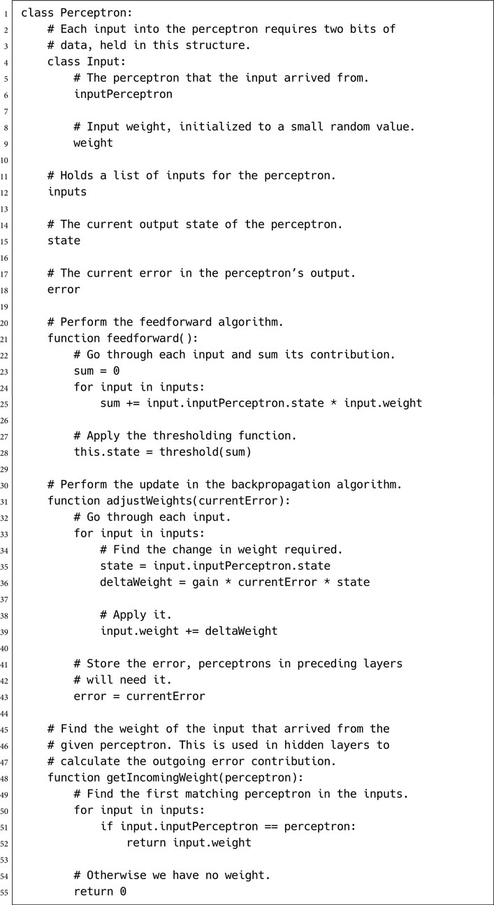
In this code I’ve assumed the existence of a threshold function that can perform the thresholding. This can be a simple ReLU function, implemented as:

To support other kinds of thresholding (such as the sigmoid function described above, or the radial basis function described later), we can replace this with a different formula.

The code also makes reference to a gain variable, which is the global gain term for the network.

7.8.6  IMPLEMENTATION CAVEATS

In a production system, it would be inadvisable to implement getIncomingWeight as a sequential search through each input. Most times connection weights are arranged in a data array. Neurons are numbered, and weights can be directly accessed from the array by index. However, the direct array accessing makes the overall flow of the algorithm more complex. The pseudo-code illustrates what is happening at each stage. The pseudo-code also doesn’t assume any particular architecture. Each perceptron makes no requirements of which perceptrons form its inputs.

Beyond optimizing the data structures, neural networks are intended to be parallel. We can make huge time savings by changing our implementation style. By representing the neuron states and weights in separate arrays, we can write both the feedforward and backpropagation steps using single instruction multiple data (SIMD) operations (such as those provided on a graphics card). Not only are we working on four neurons at a time, per processing core, but we are also making sure that the relevant data are stored together. For larger networks it is almost essential to use a graphics card implementation, taking advantage of the hardware’s many cores and massive parallelization.

7.8.7  PERFORMANCE

The algorithm is O(nw) in memory, where n is the number of perceptrons, and w is the number of inputs per perceptron. In time, the performance is also O(nw) for both feedforward (generateOutputs and backpropagation (backprop). I have ignored the use of a search in the getIncomingWeights method of the perceptron class, as given in the pseudo-code. As we saw in the implementation caveats, this chunk of the code will normally be optimized out.

7.8.8  OTHER APPROACHES

There are many books as big as this filled with neural network theory, I can’t hope to discuss it all. But most of the approaches would be of only marginal use to games. By way of a roundup and pointers to other fields, I think it is worth talking about three other techniques: radial basis functions, weakly supervised learning, and Hebbian learning. The first two I’ve used in practice, and the third is a beloved technique of a former colleague.

Radial Basis Function

The threshold function I introduced earlier is called the ReLU basis function. A basis function is simply a function used as the basis of an artificial neuron’s behavior.

The action of a ReLU basis function is to split its input into two categories. High values are given a high output, and low values are given zero output. The dividing line between the two categories is always at zero input. The function is performing a simple categorization. It distinguishes high from low values.

Figure 7.23: Bias and the sigmoid basis function

So far I’ve included the bias weight as part of the sum before thresholding. This is sensible from an implementation point of view. But we can also view the bias as changing where the dividing line is situated. For example, let’s take a single perceptron with a single input.

To illustrate (because it bears more similarity to the radial basis function I will introduce in a moment), I will return to the alternative sigmoid basis function. Figure 7.23 (left) shows the output from a perceptron when the bias is zero. Figure 7.23 (right) shows the same output from the same perceptron when the bias is one. Because the bias is always added to the weighted inputs, it skews the results.

This is deliberate, of course. You can think of each neuron as something like a decision node in a decision tree: it looks at an input and decides which of two categories the input is in. It makes no sense, then, to always split the decision at zero. We might want 0.5 to be in one category and 0.9 in another. The bias allows us to divide the input at any point.

But categorizations can’t always be made at a single point. Often, it is a range of inputs that we need to treat differently. Only values within the range should have an output of one; higher or lower values should get zero output. A big enough neural network can always cope with this situation. One neuron acts as the low bound, and another neuron acts as the high bound. But it does mean you need all those extra neurons.

Radial basis functions (first described in [6]) address this issue by using the basis function shown in Figure 7.24.

Here the range is explicit. The neuron controls the range, as before, using the bias weight. The spread (the distance between the minimum and maximum input for which the output is > 0.5) is controlled by the overall size of the weights. If the input weights are all high, then the range will be squashed. If the weights are low, then the range will be widened. By altering the weights alone (including the bias weight), any minimum and maximum values can be learned.

Radial basis functions can have various mathematical definitions. Most appear as in the figure above, a combination of a mirrored pair of sigmoid basis functions. Like the sigmoid function, they can also be very slow to learn, but conversely for some problems they fit the data more closely, allowing your network to be much smaller and more efficient.

Figure 7.24: The radial basis function

Weakly Supervised Learning

The algorithm above relies on having a set of examples. The examples can be hand built or generated from experience during the game.

Examples are used in the backpropagation step to generate the error term. The error term then controls the learning process. This is called supervised learning: we are providing correct answers for the algorithm.

An alternative approach used in online learning is weakly supervised learning (sometimes called unsupervised learning, although strictly that is something else). Weakly supervised learning doesn’t require a set of examples. It replaces them with an algorithm that directly calculates the error term for the output layer.

For instance, consider the tactical neural network example again. The character is moving around the level, making decisions based on its nearby friends and enemies. Sometimes the decisions it makes will be poor: it might be trying to heal a friend when suddenly an enemy attack is launched, or it might try to find pick-ups and wander right into an ambush. A supervised learning approach would try to calculate what the character should have done in each situation and then would update the network by learning this example, along with all previous examples.

A weakly supervised learning approach recognizes that it isn’t easy to say what the character should have done, but it is easy to say that what the character did do was wrong. Rather than come up with a solution, it calculates an error term based on how badly the AI was punished. If the AI and all its friends are killed, for example, the error will be very high. If it only suffered a couple of hits, then the error will be small. We can do the same thing for successes, giving positive feedback for successful choices.

The learning algorithm works the same way as before, but uses the generated error term for the output layer rather than one calculated from examples. The error terms for hidden layers remain the same as before.

I have used weakly supervised learning to control characters in a game prototype. It proved to be a simple way to bootstrap character behavior and get some interesting variations without needing to write a large library of behaviors.

Weakly supervised learning has the potential to learn things that the developer doesn’t know. This potential is exciting admittedly, but it has an evil twin. The neural network can easily learn things that the developer doesn’t want it to know—things that the developer can plainly see are wrong. In particular, it can learn to play in a boring and predictable way. Earlier I mentioned the prospect of a character making a last stand when the odds were poor for its survival. This is an enjoyable AI to play against, one with personality. If the character was learning solely based on results, however, it would never learn to do this; it would run away. In this case (as with the vast majority of others), the game designer knows best.

Hebbian Learning

Hebbian learning is named after Donald Hebb, who proposed in 1949 [22] that biological neurons follow this learning rule. It is still not clear how much, if any, of a biological neural network conforms to Hebb’s rule, but it is considered one of the most biologically plausible techniques for artificial neural networks. It has also proven to be practical, and is surprisingly simple to implement.

It is an unsupervised technique. It requires neither examples nor any generated error values. It tries to categorize its inputs based only on patterns it sees.

Although it can be used in any network, Hebbian learning is most commonly used with a grid architecture, where each node is connected to its neighbors (see Figure 7.25).

Neurons have the same non-learning algorithm as previously. They sum a set of weighted inputs and decide their state based on a threshold function. In this case, they are taking input from their neighbors rather than from the neurons in the preceding layer.

Hebb’s learning rule says that if a node tends to have the same state as a neighbor, then the weight between those two nodes should be increased. If it tends to have a different state, then the weight should be decreased.

The logic is simple. If two neighboring nodes are often having the same states (either both on or both off), then it stands to reason that they are correlated. If one neuron is on, we should increase the chance that the other is on also by increasing the weight. If there is no correlation, then the neurons will have the same state about as often as not, and their connection weight will be increased about as often as it is decreased. There will be no overall strengthening or weakening of the connection. This is called Hebb’s Rule.

Hebbian learning is used to find patterns and correlations in data, rather than to generate output. It can be used to regenerate gaps in data.

For example, Figure 7.26 shows a side in an RTS with a patchy understanding of the structure of enemy forces (because of fog-of-war). We can use a grid-based neural network with Hebbian learning. The grid represents the game map. If the game is tile based, it might use 1, 4, or 9 tiles per node.

Figure 7.25: Grid architecture for Hebbian learning

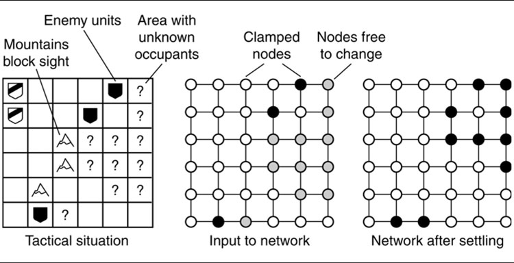
Figure 7.26: Influence mapping with Hebbian learning

The state of each neuron indicates whether the corresponding location in the game is safe or not. With full knowledge of many games, the network can be trained by giving a complete set of safe and dangerous tiles each turn (generated by influence mapping, for example—see Chapter 6, Tactical and Strategic AI).

After a large number of games, the network can be used to predict the pattern of safety. The AI sets the safety of the tiles it can see as state values in the grid of neurons. These values are clamped and are not allowed to change. The rest of the network is then allowed to follow its normal sum-and-threshold algorithm. This may take a while to settle down to a stable pattern, but the result indicates which of the non-visible areas are likely to be safe and which should be avoided.

7.9  DEEP LEARNING

From the mid-2010s onward, deep learning made it from an academic field into a media sensation. With prominent research promoted out of companies such as Google, and Deep Mind (later acquired by Google), the term became synonymous with AI. So much so that it can be difficult, outside of the specialist AI literature, to get a straight answer on what deep learning really is. It remains to be seen whether this popularity translates into longevity; or whether—as in previous cycles of AI—there follows a period of disillusionment when the limits of the technique become clear.

As an engineering approach, deep learning is strikingly powerful. It is an active area of research in many games development studios, and I would be surprised if applications in games do not follow in the coming years. Where it will be most useful, however, is less clear. Like all AI techniques (such as expert systems, or the original interest in neural networks), understanding the mechanism helps put the technique in context. It is such an active and rapidly changing area of research, and there is such voluminous literature, I cannot hope to give anything more than an overview in this book. A next step would be a textbook such as [18], or the gentler overview in Jeff Heaton’s AI for humans series [21].

7.9.1  WHAT IS DEEP LEARNING?

So far we have seen in this chapter examples of artificial neural networks that are shallow. They have only a few layers of neurons between their output and input. The multi-layer perceptron was shown with a single hidden layer, though because its output perceptions are also adaptive, it has two in total. The Hebbian network in the previous section consists of only a single layer.

A deep neural network has more layers. There isn’t an accepted criteria for how many, for when shallow become deep, but deep neural network models may have half a dozen or more. Unlike multi-layer perceptrons, in some network architectures it isn’t easy to say exactly what a layer is (recurrent neural networks, where there are loops, for example). Depending how you count, there may be hundreds or thousands.

Though deep learning is almost synonymous with neural networks, it is not entirely so. Other adaptive processes can be used (such as the decision tree learning we saw earlier in this chapter), or other algorithms used alongside neural network learning (such as Monte Carlo Tree Search in board game playing AI). The vast majority of the work in the area, however, is based on artificial neural networks, even if it draws in other techniques. I will focus on deep neural networks in this overview.

Figure 7.27: A schematic representation of a deep learning system

Figure 7.27 shows a schematic representation of a deep learning system. Each layer may consist of any kind of parameterizable structure, whether an array of perceptrons, an image filter (also known as a convolution, from which convolutional neural networks get their name), even a probabilistic model of human language (used in speech recognition and translation). For the system to be deep, it succeeds or fails as a whole. Which in turn means a learning algorithm must be applied to the whole. All the parameters in all the layers are changed during learning. In practical applications, there may be a combination of this global parameterization, and some local changes presided over by local learning algorithms (sometimes known as a greedy layer-by-layer approach), but it is the overall global learning that makes the system ‘deep’.

7.9.2  DATA

In Section 7.8, above, I described the credit assignment problem (CAP). The network is run, an output is generated, and the output is judged for quality. For supervised learning this involves a list of known correct examples to compare to. For weakly or unsupervised learning it may mean testing the output in practice and seeing if it succeeds or fails. In either case, to learn, we need to be able to work backwards from the score and from the parameters which generated it, to a new set of parameters, which hopefully will do better. The problem of determining which parameters to change is the credit assignment problem. The number of layers of parameters to change is known as the credit assignment path depth. For decades it was generally thought that learning a deep CAP was simply intractable. This changed in the early 2010s for three reasons:

1.  new techniques in neural networks were developed, such as using the ReLU function rather than the sigmoid function for perceptrons, or ‘dropout’: resetting neurons at random during backpropagation;

2.  computer power increased, partly in the way Moore’s law predicted, but particularly with the availability of highly parallel and affordable GPU computing;

3.  larger data sets became available due to large-scale indexing of the web, and more autonomous tools for information gathering in biotechnology.

For games, it is often the last of these three which limits the ability to use deep learning. Deep learning has a lot of parameters to change, and successful learning requires considerably more data than parameters. Consider the situation shown in Figure 7.28. Here we are trying to determine threatening enemies. I have deliberately simplified the situation to fit in a diagram. There are eight scenarios, each labeled whether it is threatening or not. Figure 7.29 shows the network we are using to learn: it has eight nodes in its intermediate layer (for simplicity it is shown as a shallow neural network, if it had a dozen layers the problem would be even more acute).

After learning until the network can correctly classify the situations given, the scenario in Figure 7.30 is presented to the network. It is as likely as not to incorrectly classified this situation. This is not a failure in the learning algorithm, or a mistake in implementation. The data is sparse enough that each neuron in the hidden layer simply learned the correct answer to one input scenario. When a new test is presented, the amount of generalizing the network can do is minimal, the output is effectively random. The network is said to have over-fitted the data. It has learned the input rather than the general rule.

The more parameters to learn, the more data is needed. This can be a problem if you are relying on manually labeled data sets, or if testing the neural network involves playing a game, or simulating part of a game. One of the breakthroughs of deep learning, described in [32], achieved a roughly $\frac{2}{3}$ success rate on the 1.2 million hand labeled ImageNet corpus, using a network with 650,000 neurons in five layers. Acquiring and validating that much data for the character AI in a game is difficult, and a success rate of $\frac{2}{3}$ is unlikely to be impressive to players used to finding and exploiting failures.

Figure 7.28: Situations for which to learn a strategic threat assessment

Figure 7.29: The neural network learning a strategic threat assessment

Figure 7.30: A failed strategic threat assessment with a fully trained network

EXERCISES

7.1  Chapter 3, Section 3.5.1, discussed aiming and shooting. How might we use hill climbing to determine a firing solution?

7.2  Implement a hill climbing approach to determining a firing solution for some simple problems.

7.3  In terms of both speed and accuracy, compare the results you obtain from your implementation for Exercise 7.2 to solutions obtained analytically from the equations given in Chapter 3. Use your results to explain why, for many problems, it might not make sense to use hill climbing or any other learning technique to discover a firing solution?

7.4  Suppose an AI character in a game can direct artillery fire onto a battlefield. The character wants to cause explosions that maximize enemy losses and minimize the risk to friendly units. An explosion is modeled as a circle with a fixed deadly blast radius r. Assuming the location of all enemy and friendly units is known, write down a function that calculates the expected reward of an explosion at a 2D location (x, y).

7.5  If you didn’t already, modify the function you wrote down for Exercise 7.4 to take into account the potential impact on morale of friendly fire incidents.

7.6  Explain why simple hill climbing might not find the global optimum for the function you wrote down for Exercise 7.4. What techniques might you use instead?

7.7  Many fighting games generate special moves by pressing buttons in a particular order (i.e., “combos”). For example, “BA” might generate a “grab and throw” and “BAAB” might generate a “flying kick.” How could you use an N-Gram to predict the player’s next button press? Why would using this approach to create opponent AI probably be a waste of time? What applications might make sense?

7.8  In some fighting games a combo performed when the character being controlled is in a crouching position will have a different effect than when the character is standing. Does the approach outlined in Exercise 7.7 address this point? If not, how could it be fixed?

7.9  Suppose you have written a game that includes a speech recognizer for the following set words: “go,” “stop,” “jump,” and “turn.” Before the game ships, during play testing, you count the frequencies with which each word is spoken by the testers to give the following table:

Word	Frequency
“go”	100
“stop”	125
“jump”	25
“turn”	50

Use these data to construct a prior for P (word).

7.10  Carrying on from Exercise 7.9, further suppose that, during play testing, you timed how long it took players to say each word and you discovered that the time taken was a good indicator of which word was spoken. For example, here are the conditional probabilities, given the word the player spoke, that it took them more than half a second:

Word	P(length(signal) > 0.5|word)
“go”	0.1
“stop”	0.05
“jump”	0.2
“turn”	0.1

Now suppose that, during gameplay, we time how long it takes a player to utter a word. What is the most likely word the player spoke, given that it took 0.9 seconds to say it? What is its probability? (Hint: Apply Bayes rule:

$P\left(A|B\right)=\alpha P\left(B|A\right)P\left(A\right)$

where α is a normalizing constant, then use the prior you constructed in Exercise 7.9 and the given conditional probabilities.)

7.11  Suppose we are trying to learn different styles of playing a game based on when a player decides to shoot. Assume the table below represents data that we have gathered on a particular player:

shoot?	distance-to-target	weapon-type
Y	2.4	pistol
Y	3.2	rifle
N	75.7	rifle
Y	80.6	rifle
N	2.8	pistol
Y	82.1	pistol
Y	3.8	rifle

Using a suitable discretization/quantization of distance-to-target, fill out a new table of data that will be easier to learn from:

shoot?	distance-to-target-discrete	weapon-type
Y		pistol
Y		rifle
N		rifle
Y		rifle
N		pistol
Y		pistol
Y		rifle

7.12  Using the new table of data you filled out in Exercise 7.11 assume we want to construct a Naive Bayes classifier to decide whether an NPC should shoot or not in any given situation. That is, we want to calculate:

$P\left(\text{shoot?}|\text{distance}-\text{to}-\text{target}-\text{discrete, weapon}-\text{type}\right)$

(for shoot? = Y and shoot? = N) and pick the one that corresponds to the larger probability.

7.13  In Exercise 7.12 you only had to calculate the relative conditional probabilities of shooting versus not shooting, but what are the actual conditional probabilities? (Hint: Remember that probabilities have to sum to 1.)

7.14  In Exercise 7.12 we made the assumption that, given the shoot action, the distance to the target and the weapon type are conditionally independent. Do you think the assumption is reasonable? Explain your answer.

7.15  Re-implement the Naive Bayes classifier class given in Section 7.5 using logarithms to avoid floating-point underflow problems.

7.16  Suppose we have a set of examples that look like the following:

Use information gain to build a decision tree from the examples.

7.17  Write down a simple rule that corresponds to the decision tree you built for Exercise 7.12. Does it make any sense?

7.18  Implement the obstacle avoidance behavior described in Section 3.3.15 and use it to generate some data. The data should record relevant information about the environment and the character’s corresponding steering choices.

7.19  Take a look at the data you generated from working on Exercise 7.18. How easy do you think the data are to learn from? How could you represent the data to make the learning problem as tractable as possible?

7.20  Use the data you generated from working on Exercise 7.18 to attempt to learn obstacle avoidance with a neural network. The problem is probably harder than you imagine, so if it fails to work try re-visiting Exercise 7.19. Remember that you need to test on setups that you didn’t train on to be sure it’s really working.

7.21  Obstacle avoidance naturally lends itself to creating an error term based on the number of collisions that occur. Instead of the supervised approach to learning obstacle avoidance that you tried in Exercise 7.20, attempt a weakly supervised approach.

7.22  Instead of the weakly supervised approach to learning obstacle avoidance that you tried in Exercise 7.21, try a completely unsupervised reinforcement learning approach. The reward function should reward action choices that result in collision-free movement. Remember that you always need to test on setups that you didn’t use for training.

7.23  Given that reliable obstacle avoidance behavior is probably far easier to obtain by hand coding, is trying to use machine learning misguided? Discuss the pros and cons.