5.4 Forwarding Priority Scheduling

In this section, we will answer the question “in the time fraction λα assigned to Tα, how can we schedule the forwarding priorities among the forwarding candidates of the transmitter to satisfy ?” Note that is the normalized link rate over the whole scheduling period, thus, during the time fraction λα, the link rate on is . For simplicity, we denote as ni, and as in the following discussion. Furthermore, we denote the rate vector as , where . The forwarding priority scheduling problem (FPSP) can therefore be formally defined as follows:

Definition 5.1 FPSP: Given , find a forwarding priority scheduling , such that on link , the accumulated effective rate .

In the definition, and βm are the mth forwarding priority and its time fraction, respectively. So βm ≥ 0 , and . L is the total number of different priority assignment. Under the scheduling, can be computed as follows:

5.18

where is the effective forwarding rate on link defined in Equation (5.7) under the forwarding priority .

5.4.1 A Scheduling Based on LP

One way to get a scheduling of opportunistic forwarding priorities for a rate vector is by solving a linear programming problem in Figure 5.3. The basic idea of this linear programming is to enumerate all possible r! opportunistic forwarding priorities to see if we can find a feasible solution. If the solution of the objective function (5.19) is no greater than 1, then the flow vector is schedulable, and is a feasible scheduling; otherwise, the flow vector is not schedulable.

The linear programming in Figure 5.3 provides a way to judge the schedulability of a rate vector corresponding to an opportunistic module and find a schedule of forwarding priorities if the rate vector is schedulable. At most, r is the number of all the one-hop neighbors of a transmitter, so it tends to be a relatively small number. However, it may not be necessary to enumerate all the possible forwarding priorities to find a feasible scheduling. In the following subsection, we propose a heuristic algorithm to solve the FPSP in a more efficient way.

5.4.2 A Heuristic Scheduling

Table 5.1 describes the heuristic recursive algorithm that finds a schedule of opportunistic forwarding priorities satisfying the rate vector . The basic idea of this algorithm is to satisfy each rate one-by-one by using two priority settings: assigning the corresponding candidate the highest and lowest priority in the existing subset of the candidates. In the algorithm, we take advantage of the property of OR that the effective forwarding rate of a lower-priority candidate is not affected by the priority relationships among the higher priority candidates. Then we can consider a group of forwarding candidates as a virtual candidate, whose PRR is the probability of at least one forwarding candidate receiving the packet correctly, and the rate to this virtual candidate can be computed using Equation (5.8).

Table 5.1 Pseudocode of a heuristic recursive algorithm for finding a scheduling of opportunistic forwarding strategies

In Table 5.1, the input of the prioritizing and scheduling algorithm PS includes: , the rate vector; , the corresponding PRR vector; , the corresponding forwarding candidate index vector; r, the number of candidates; β, the active time fraction of the links corresponding to candidates in ; ω, a scalar on the PRR, which is used to calculate time fraction β1 and β2 in line 7. Initially, β = ω = 1. The output of this algorithm is a set of opportunistic forwarding priorities, S, and the corresponding time fraction vector, Γ.

Lines 1 and 2 indicate the basic case where there is only one candidate; then the candidate index and the corresponding time fraction β are returned. When the number of candidates is larger than 1, we first pre process the rate vector (in lines 4 and 5) such that if there is a rate equal to its corresponding scaled PRR timing the transmission rate or no greater than the scaled effective forwarding rate when the corresponding candidate is assigned the lowest priority, we put this candidate at the first place of the candidate vector. We then split the candidates into two parts, part 1: I1 and part 2: [I2…Ir]. Next, we calculate the accumulated PRR P2 of candidates [I2…Ir]. In line 7, we calculate the time fractions β1 and β2 corresponding to prioritization 〈I1, [I2…Ir]〉 and 〈[I2…Ir], I1〉, respectively. Note that 〈I1, [I2…Ir]〉 indicates the candidate I1 has higher relay priority than the group of candidates [I2…Ir], and vice versa. Then we recursively call the function PS on I1 and [I2…Ir] (in lines 8 to 11). The returned Sij is the set of forwarding strategies when part i is in the jth place (j = 1, 2 indicates higher and lower priority, respectively). Then we combine the sequences in S11 and S22 to get S1 which are sequences of candidates with I1 having higher priority than [I2…Ir] (in line 12). Similarly, we combine S21 and S12 with group of candidates [I2…Ir] having higher priority than I1 (in line 13). Finally, we return the whole series of prioritizations by taking the union of S1 and S2.

Next, we explain the Merge algorithm in Table 5.2. We assume both input (S1, S2, Γ1 and Γ2) and output (S and Γ) are stored in stacks. The basic idea of this Merge algorithm is to concatenate the sequence (corresponding to a prioritization) in the top of S1 with that in the top of S2 (in line 3) to create a new sequence (prioritization). The time fraction of this new sequence is the minimum of the time fractions of these two subsequences. After creating a new sequence, we pop the sequence with smaller time fraction, and update the time fraction of the other sequence by subtracting the used time fraction (in lines 5, 7, and 9). When all the sequences in S1 and S2 are popped out, a series of new sequences S and the corresponding time fraction vector Γ are returned (in line 11).

Table 5.2 Pseudocode of merging two prioritized sub-sets of candidates

The computation complexity of Merge algorithm is Θ(|S1| + |S2|), where |Si| (i = 1, 2) is the number of sequences in Si. For Si with x elements, we have at most O(2x) and at least Ω(1) sequences in it. So the complexity of the algorithm PS is O(2r−1) in the worst case and Ω(r) in the best case, where r is the number of forwarding candidates.

5.4.2.1 Correctness of the Heuristic Algorithm

This heuristic algorithm does not guarantee to return a feasible schedule of opportunistic forwarding priorities even when the rate vector is schedulable. When this happens, we need to run the LP in Figure 5.3 to get a feasible scheduling. However, we will prove that this heuristic algorithm does return a feasible scheduling for a schedulable rate vector when r ≤ 2. We will also show numerical results that this heuristic algorithm works well for larger number of forwarding candidates in terms of achieving low unsatisfied rate ratio.

Proposition 5.1 When is no greater than 2, any rate vector in the capacity region defined in Inequality (5.9) can be satisfied by the scheduling obtained by the heuristic algorithm PS in Table 5.1.

Proof. First, when r = 1, it is obvious that any μ1, s.t. , is schedulable. Lines 1 and 2 in Table 5.1 deal with this case.

Second, when r = 2, there are two forwarding priorities: and . Assuming the whole transmission period is unit 1, we allocate β1 and β2 time fraction for and , respectively. Then according to Equation (5.18), we have

5.22

5.23

Then we only need to prove, for any μ1 and μ2, s.t. , 0 ≤ μ2 ≤ Ri, and μ1 + μ2 ≤ Ri(1 − (1 − )(1 − )), β1 and β2, s.t. 0 ≤ β1 ≤ 1, 0 ≤ β2 ≤ 1, and β1 + β2 = 1, to make and μ2 ≤ .

With μ2 ≤ , μ2 ≤ Ri, Equation (5.23) and β1 = 1 − β2, we have

5.24

With μ1 ≤ , μ1 ≤ Ri, Equation (5.22) and β2 = 1 − β1, we have

5.25

By satisfying μ1, we set

5.26

By substituting Equation (5.26) into Equations (5.22) and (5.23), we can verify that μ1 ≤ and μ2 ≤ . Note that, the setting of β1 and β2 makes inequalities (5.24) and (5.25) hold. Equation (5.26) exactly corresponds to the first two equations in line 7 in Table 5.1. So we proved the correctness of the heuristic algorithm PS for r = 2.

The proof of the correctness of the heuristic algorithm also indicates that any rate vector in the capacity region shown in Figure 5.4 is schedulable.

Figure 5.4 Capacity region for two forwarding candidates. Reproduced by permission of © 2010 IEEE.

5.4.2.2 An Example

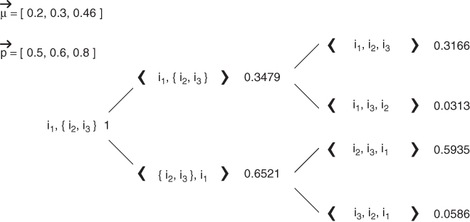
We use an example to illustrate how the PS algorithm works. Assume ni has three forwarding candidates , the corresponding rate on each link (q = 1, 2, 3) is 0.2Ri, 0.3Ri, and 0.46Ri, and the corresponding PRR on these links are 0.5, 0.6 and 0.8, respectively. Figure 5.5 shows the running result of algorithm PS. In the first stage, μ1 is satisfied, and in the second stage μ2 is satisfied, then μ3. The time fraction β of each forwarding priority is listed at the right of the priority.

Figure 5.5 An example of opportunistic forwarding strategy scheduling for three forwarding candidates. Reproduced by permission of © 2010 IEEE.

5.4.2.3 Performance of the Heuristic Algorithm

We conducted numerical simulations to evaluate the performance of the PS algorithm. We propose the metric of unsatisfied rate ratio γ to indicate how well the heuristic algorithm can satisfy the rate vector .

5.27

where is the accumulated effective rate on link defined in Equation (5.18) under a scheduling of forwarding priorities, and I() is an indicator function. When the input expression of I() is true, I() = 1; otherwise I() = 0. According to Equation (5.27), 0 ≤ γ ≤ 1. A smaller γ indicates better performance.

In the simulation, we vary the number of forwarding candidates from 1 to 10. For each number of forwarding candidates, we conducted 104 runs. In each run, we randomly assign the PRR on the links in the opportunistic module, and generates a rate vector that reaches the capacity of that opportunistic module. Then we run PS algorithm on the rate vector and opportunistic module, and compute the corresponding γ. Figure 5.6 shows the mean of γ with 95% confidence interval under different number of forwarding candidates. We can see that the PS algorithm works well in terms of having low γ. It satisfies the rate vector almost all the time with the unsatisfied ratio as low as 0.7% when there are no more than five forwarding candidates. When the number of forwarding candidates increases, γ is increased. However, even when there are ten forwarding candidates, γ is below 10%.

Figure 5.6 Unsatisfied rate ratio versus number of forwarding candidates using PS algorithm for forwarding priority scheduling. Reproduced by permission of © 2010 IEEE.