In this section, we use Matlab to investigate the impact of different factors on the end-to-end throughput bound of opportunistic routing, such as source–destination distances, node densities, and number of forwarding candidates. Both line and square topologies are studied for each factor. We also compare the performance of single rate opportunistic routing and multirate ones, and the performance of OR with traditional routing (TR). We call a routing scheme “traditional” when there is only one forwarding candidate selected for each packet relay at each hop.
The OR schemes we investigate include single-rate ExOR (Biswas and Morris 2005), single/multirate GOR and single/multirate LMTOR introduced in Section 4.3.1. For ExOR (Biswas and Morris 2005), each transmitter selects the neighbors with lower ETF (Expected number of Transmissions over Forward links) to the destination than itself as the forwarding candidates, and neighbors with lower ETF have higher relay priorities. For GOR, the forwarding candidates of a transmitter are those neighbors that are closer to the destination, and candidates with larger advancement to the destination have higher relay priorities. The EAR metric proposed in Section 4.2 is used to select the transmission rate for each node in the multirate scenario. For multirate LMTOR, the algorithm and metric proposed in Section 4.3.1 is used to choose transmission rate and forwarding candidates at each node. All the evaluations are under protocol model.
4.4.1 Simulation Setup
The simulated network has 20 stationary nodes randomly uniformly distributed on a line with length L or in a W × Wm2 square region. The data rates 24, 12, and 6 mbps (chosen from 802.11a) are studied. We use one of the most common models–log-normal shadowing fading model (Rappaport 1996) to characterize the signal propagation. The received signal power is:
where Pr(d)dB is the received signal power at distance d from the transmitter, β is the path loss exponent, and XdB is a Gaussian random variable with zero mean and standard deviation σdB. Pr(d0)dB is the receiving signal power at the reference distance d0, which is calculated by Equation (4.18):
where Pt is the transmitted signal power, Gt and Gr are the antenna gains of the transmitter and the receiver respectively, c is velocity of light, f is the carrier frequency, and L is the system loss.
In our simulation, d0 = 1 m, β = 3, σdB = 6, Gt, Gr and L are all set to 1, Pt = 15 dbm, c = 3 × 10⁸ m/s, and f = 5 GHz.
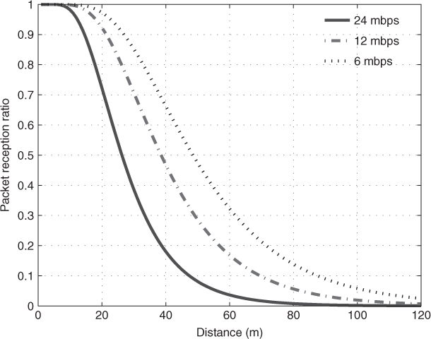
We assume a packet is received successfully if the received signal power is greater than the receiving power threshold (PTh). According to Yee and Pezeshki-Esfahani (2002), for 802.11a, the PTh for 24, 12, and 6 mbps is −74, −79, and −82 dbm, respectively. Then according to Equations (4.17) and (4.18), the packet reception ratio for each rate at a certain distance d can be derived. The PRR versus distance for each data rate is shown in Figure 4.4. We set the PRR threshold ptd as 0.1, so the effective transmission radius for each rate (24, 12, and 6 mbps) is 47, 70 and 88 m, respectively. As discussed in Zhai and Fang (2006b), 802.11 systems have very close interference ranges for different channel rates, so we use a single interference range 120 m for all channel rates for simplicity.
Figure 4.4 Packet reception ratio versus distance at different data rates.
4.4.2 Impact of Source–Destination Distances
In this subsection, we evaluate the impact of the source–destination distance on the end-to-end throughput bound of OR and TR in line and square topologies. For line topology, the length L is set as 400 m. We fix the left-end node as the destination, and calculate the throughput bounds from all other nodes to it under different OR and TR variants. For square topology, the side length is set as 150 m. We fix the node nearest to the lower left corner as the destination, and calculate the throughput bounds from all other nodes to it. Therefore, there are 19 different source–destination pairs considered in the evaluation for each topology. We evaluate the performance under both single-rate and multirate scenarios. The average numbers of neighbors per node (indicated as ρ) under different topologies and data rates are summarized in Tables 4.1.
Table 4.1 Average number of neighbors per node under different topologies and data rates.
| ρ | ||
| Rate (mbps) | Line | Square |
| 24 | 3.5 | 3.5 |
| 12 | 5.5 | 7.0 |
| 6 | 6.8 | 10.0 |
In the single-rate scenario, for TR, we compute the exact end-to-end throughput bound between the source–destination pairs according to the LP formulations in (Jain et al. 2003), which normally result in multiple paths from the source to the destination. So we call it “Multipath TR”. We also compute the end-to-end throughput of a single path that is found by minimizing the medium time (delay), and we call it “Single-path TR”. The bound of single-path TR is calculated according to the formulations in (Zhai and Fang 2006a). For the three OR variants, we compute the throughput bounds under both conservative (indicated as “c”) and greedy (indicated as “g”) modes as we discussed in Section 4.1.2.
Figure 4.5 shows the simulation results of LMTOR, ExOR, GOR and TR in a single rate (12 mbps) system under line topology. We have the following observations: 1. when the distance between the source and destination increases, the end-to-end throughput bound of each routing scheme decreases. 2. the OR achieves higher throughput bound than TR under different source–destination distances. 3. all the OR variants achieve the same performance under the same mode. 4. when source–destination distance is larger than two hops, OR in greedy mode results in higher end-to-end throughput than that in conservative mode, whereas when the source–destination distance is smaller than two hops they represent the same performance. 5. the multipath TR achieves almost the same throughput bound as single-path TR.
Figure 4.5 End-to-end throughput bound of OR and TR in a single rate (12 mbps) network under line topology. Reproduced by permission of © 2008 IEEE.

In the line topology, the throughput gain of OR over TR mainly comes from the opportunistic property. That is, for each packet transmission, multiple forwarding candidates help on forwarding the packet. The reliability of at least one forwarding candidate correctly receiving the packet is increased comparing to TR. The increased reliability reduces the retransmission overhead and saves the medium time for each packet forwarding, thus improving the throughput.
By tracing into the simulation, we find that the three OR variants result in the same forwarding candidate selection and prioritization at each forwarding node, although they follow different criteria to select the candidates and prioritize them. That's why we have the observation 3, which indicates that in the line topology the per-hop greedy behavior in GOR can approach the same end-to-end performance as that obtained by a distributed scheme like LMTOR.
For the observation 4, when the source is near to the destination, all the nodes along the paths are in the interference range of each other, thus there is no concurrent transmission allowed in either greedy or conservative mode. Therefore, OR in both modes achieves the same performance when the source–destination distance is smaller than two hops. When the source–destination distance is lager than two hops, concurrent transmission in the network becomes possible. Since the conservative mode requires interference-free communication at all the forwarding candidates, for each transmission, it consumes more space than the greedy mode, which only needs interference-free communication at least at the forwarding candidate. That is, the greedy mode achieves a higher spacial reuse ratio than conservative mode and allows more concurrent transmissions in the network, thus resulting in higher throughput.
The observation 5 indicates that multipath TR does not really improve the wireless network throughput over the single-path TR in the line topology. The reason is that even when there are multiple paths between the source and destination, the links on different paths cannot be scheduled at the same time due to interference. Opportunistic routing does make real use of multiple paths in the sense that throughput can take place on any one of the outgoing links from the sender to its forwarding candidates.
Figure 4.6 shows the simulation results of LMTOR, ExOR, GOR and TR in a single rate (12 mbps) system under square topology. One interesting observation is that the multipath TR achieves (up to 60%) higher throughput bound than single-path TR, and it can achieve comparable or even higher throughput than OR in conservative mode when the source–destination distance is larger than two hops. In the square topology, when the source and destination are far apart, real multipath routing becomes feasible. That is, different links on different paths can be activated at the same time and this improves the throughput. This observation also indicates that it is not a good idea to include as many forwarding candidates as possible into opportunistic routing when a protocol requires freedom from interference at all the forwarding candidates. As we can see in Figure 4.6 OR in greedy mode still achieves higher throughput than OR in conservative mode and multipath TR. So the advantage of OR over TR is still validated.
Figure 4.6 End-to-end throughput bound of OR and TR in a single rate (12 mbps) network under square topology. Reproduced by permission of © 2008 IEEE.

Opportunistic routing in greedy mode always achieves higher throughput bound than that in conservative mode, so in the following evaluation, the throughput bound of OR is only calculated under greedy mode. As the performance of ExOR is nearly the same as that of GOR, we will not show the simulation result of ExOR in the following figures. Now, we compare the throughput bounds of OR in multirate and single-rate systems.
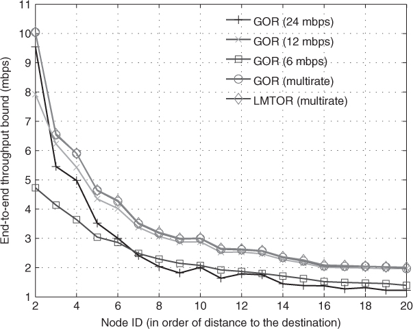
Figure 4.7 shows the simulation results of multirate LMTOR, multirate GOR, and single-rate GOR under line topology. We can see that generally multirate OR achieves better performance than any single-rate OR. When the distance between the source and destination is shorter than the interference range (corresponding to node ID 7), the system operating on 24 mbps achieves better performance than that on 12 mbps. However, the difference becomes smaller and smaller when the source–destination distance becomes larger, since more forwarding candidates are involved for 12 mbps and the spacial diversity is increased. When the source–destination distance is larger than the interference range, the performance of 24 mbps is the same as that of 12 mbps. Figure 4.8 shows the simulation results under square topology. An interesting difference from line topology is that the system operating at 24 mbps shows lower throughput bound than those operating at 12 mbps and 6 mbps for most of the source–destination pairs. The disadvantage of short transmission range and lower spacial diversity of 24 mbps overwhelms its higher data-rate advantage in the square topology.
Figure 4.7 End-to-end throughput bound of OR in single-rate and multirate networks under line topology. Reproduced by permission of © 2008 IEEE.

Figure 4.8 End-to-end throughput bound of OR in single-rate and multirate networks under square topology. Reproduced by permission of © 2008 IEEE.
4.4.3 Impact of Forwarding Candidate Number
In this subsection, we study the impact of the number of forwarding candidates on the performance of OR. For line topology, we examine the bound between the two end nodes on the line. For square topology, we examine the throughput bound between the two end nodes on the diagonal. The topology sizes are set as the same as those in the previous simulation. For a transmitter, given a maximum number of forwarding candidates, the single-rate GOR selects the forwarding candidates as follows: first, it finds all the neighbors that are closer to the destination than the transmitter; second, if the number of neighbors found is less than or equal to the maximum number of forwarding candidates, GOR just involves all the found neighbors and gives the neighbors closer to the destination higher relay priorities. If the number of the found neighbors is greater than the maximum number of forwarding candidates, we apply the algorithm proposed in (Zeng et al. 2007b) to select the forwarding candidates which maximizes the EPA. For multirate GOR, we select the forwarding candidates for each single-rate GOR and calculate its corresponding EAR, then select the data rate with the highest EAR. For LMTOR, we apply the distributed algorithm proposed in Section 4.3.1. For the local search in Equations (4.14) and (4.15), we only test a subset of all the neighbors with cardinality no larger than the maximum number of forwarding candidates.
Figures 4.9 and 4.10 show the simulation results under line and square topologies, respectively. Generally, multirate OR achieves better performance than any single-rate OR, and multirate LMTOR achieves better performance than multirate GOR. In the square topology (Figure 4.10), GOR on 12 mbps is always the best among all the single-rate GOR for all the different candidate sizes. The 24 mbps GOR performs even worse than the 6 mbps GOR in square topology when the maximum forwarding candidate number is larger than 3. Since 24 mbps has the shortest transmission range, which results in the lowest node density as shown in Table 4.1, GOR on 24 mbps actually does not have three or more forwarding candidates to choose. Note that, the maximum number of forwarding candidates being equal to 1 corresponds to the TR. Although 6 mbps geographic TR (GTR) achieves lower throughput bound than 24 mbps GTR, it is not necessarily the truth for GOR. Lower data rates have longer transmission ranges, so this yields higher neighborhood diversities, which can help to increase the effective forwarding rate for each transmission when OR is used. In the line topology (Figure 4.9), when the forwarding candidate number is greater than 3, GOR on 12 mbps achieves better performance than that on 24 mbps which can be explained by the same reason. However, in the line topology, the disadvantage of low data rate of 6 mbps overwhelms its advantage on higher spacial diversity, GOR on 6 mbps shows the worst performance.
Figure 4.9 End-to-end throughput bound of OR with different number of forwarding candidates under line topology. Reproduced by permission of © 2008 IEEE.

Figure 4.10 End-to-end throughput bound of OR with different number of forwarding candidates under square topology. Reproduced by permission of © 2008 IEEE.

An interesting observation in both Figure 4.9 and Figure 4.10 is the concavity of each curve, which indicates that although involving more forwarding candidates improves the end-to-end throughput bound of OR, the capacity gained becomes marginal when we keep doing so. We can see that when the number of forwarding candidates is larger than 3, the end-to-end throughput bound remains almost unchanged. This end-to-end throughput observation is consistent with the local behavior found in Chapter 2. For a realistic MAC for OR, the coordination overhead is likely to increase when more forwarding candidates are involved. Since the throughput gain decreases when the number of forwarding candidates is increased, considering the MAC overhead, it may not be wise or necessary to involve as many as forwarding candidates in OR.
4.4.4 Impact of Node Density
The impact of the node density on the performance of OR is investigated in this subsection. Instead of single flow, we investigate the multiflow case by randomly selecting four source–destination pairs in the network. The settings of the network terrain size and the corresponding number of neighbors per node under different data rates are summarized in Table 4.2 and 4.3.
Table 4.2 Average number of neighbors per node at each rate under square topology with different side lengths.

Table 4.3 Average number of neighbors per node at each rate under square topology with different side lengths.

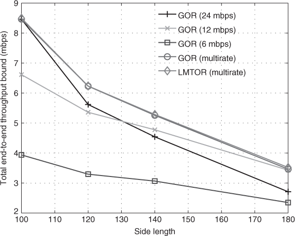
Figures 4.11 and 4.12 show the simulation results under line and square topologies, respectively. They show the same trend. There exists a threshold on the node density, higher than which the GOR on 24 mbps performs better than that on 12 mbps, and lower than which the opposite is the case. The threshold is about 5.5 and 10.9 neighbors per node on 12 mbps for line and square topologies, respectively. Our proposed multirate GOR and LMTOR can adapt to the different node densities, and choose the proper transmission rate and forwarding candidate set to achieve a better performance than any single-rate GOR.
Figure 4.11 Total end-to-end throughput bound of OR under line topology with different lengths in multiflow case.

Figure 4.12 Total end-to-end throughput bound of OR under square topology with different side lengths in multiflow case. Reproduced by permission of © 2008 IEEE.