
CHAPTER 1
Setting the Stage
OVERVIEW
This chapter defines key terms that will be used throughout the book. I start by describing fixed income securities and the size of the global fixed income markets. I introduce the term systematic and distinguish it from quantitative. All fixed income market participants are quantitatively aware; after all commonly used analytics like duration and convexity require a little more than elementary school mathematics. However, not all fixed income investors are systematic in how they translate their investment narratives into portfolios. That is what it means to be a systematic investor: prespecifying your investment hypotheses (narrative) and then converting that to an algorithm that generates trades and ultimate portfolio positions. We will explore the key ingredients of that algorithm as we proceed through the book. Finally, while this book is designed for fixed income investors and not financial engineers, resulting in minimal mathematical proofs, it is still important that commonly used analytics like yields, durations, and convexity are well understood. We will cover the intuition of these concepts, and their limitations, in detail.
1.1 WHAT IS FIXED INCOME?
This book is focused on understanding the investment opportunities available to asset owners from the fixed income markets. We need to define what makes a financial asset a fixed income security. But let's first start with a brief discussion of what a financial asset is to help set the stage for what is to come later in this chapter. All financial assets provide the owner a right to share in the cash flows generated from ownership. The price of a financial asset today will reflect expected cash flows for today, tomorrow, and all future time periods until the security ceases to exist. You don't need to hold the security to maturity to receive the actual cash flows: the price of the security will capture expectations (albeit noisily) of all future cash flows. Implicit in this last statement is an equivalence of cash flows that accrue over different time periods. Of course, there is a complicated discounting that is applied to expected future cash flows to arrive at a price. These statements are true for all financial assets, whether they be common stocks or bonds or any other contractual claim.
We can start with a simple general equation linking the price of a financial asset to its expected cash flow participation rights:
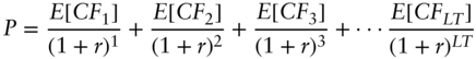
Equation 1.1 is a discrete time pricing formula generalizable to all financial assets. E[] captures expectations based on information today with respect to future cash flows, CF. These cash flows are discounted back to today, reflecting not just time value of money considerations but also perceived risk of associated cash flows. (We will have more to say on discount rates and its components throughout this book.) Fixed income securities are relatively unique, relative to equity securities, in two key respects. The key is in the name of the asset class: “fixed” income. First, the numerator is less important from a security valuation perspective (cash flows are “fixed”). Expected future cash flows for fixed income securities (the numerator) are typically known in advance, with almost complete certainty for truly risk‐free securities. Uncertainty in the numerator (one‐sided for fixed income and more two‐sided for equity) is increasing in the risk that the issuer will be unable to deliver those future cash flows (e.g., a risky corporate issuer). Generally, fixed income security pricing is dominated by the denominator. In contrast, equity securities require detailed forecasting of both the numerator and denominator for any meaningful security valuation. Some might be tempted to say fixed income investing is easier as a result. Alas, it is not; it is just that your focus is shifted to the denominator. Second, fixed income securities have limited lives, and the life of the fixed income security is typically also “fixed.” Of course, there are complexities with embedded options that can alter (usually shorten) the life of a fixed income security, but fixed income securities generally have a prespecified time to pay cash flows. This has very important implications for valuation of the cash flows. As time passes the value of the claim will change, absent any changing views of the expected cash flows. This gives rise to unique investment opportunities and challenges for fixed income securities (e.g., the importance of carry for identifying expected returns and the complications of modeling the deterministic time‐varying risk profile of fixed income securities), all of which we will cover in detail later in this book.
So where do the fixed income securities come from? Entities of various forms require capital to finance their operating and investing activities. The most common entities that issue fixed income securities are (i) governments and quasi‐government entities, and (ii) corporations. We will focus on fixed income securities from these two issuers in this book. Governments and corporations from all countries engage in debt financing across both developed and emerging markets. Our focus will be on developed markets, but there will be some discussion of the unique risks and investment opportunities in emerging market debt in Chapter 7. There is also a large set of asset‐backed fixed income securities. These are largely repackaging of other fixed income securities into pools where the cash flow rights are reassigned to new fixed income securities. Perhaps the largest securitized market is the government sponsored mortgage‐backed securities in the United States. But there are other large pools of securitized assets globally such as covered bonds issued by financial institutions (largely in Europe) and nonagency mortgages. We will have less to say on securitized assets in this book, outside of the prepayment risk premium to be discussed in Chapter 2. However, the security valuation frameworks and portfolio construction considerations we cover for the more common government and corporate fixed income securities can be tailored across the full breadth of fixed income securities.
1.2 HOW BIG ARE FIXED INCOME MARKETS?
Let's start broad when assessing the size of the potential investment opportunity set for the fixed income asset class. Although there are no universally accepted statistics for the true size of fixed income (or indeed equity) markets, the Bank for International Settlements is a commonly used reference for this purpose. Exhibit 1.1 shows the size of global fixed income markets as of December 31, 2020. Clearly, the global fixed income market is enormous, accounting for a little over $123 trillion USD. This estimate is an attempt to capture broadly investible fixed income markets. Ilmanen (2022) notes that the size of global fixed income markets could be closer to $200 trillion if all money market securities and all bank loans were included. Global equity markets, in contrast, were valued at $106 trillion USD as of December 31, 2020.1 There is clearly a concentration in debt securities in developed markets, but there is an increasing presence of Chinese domiciled issuers over the past decade.
An alternative way to understand global fixed income markets is to assess the relative importance of issuer type. Exhibit 1.2 shows that government entities (includes supranationals and quasi‐sovereign issuers) account for a little more than half of total fixed income securities outstanding. Financial institutions (inclusive of asset‐backed securities and regular bonds) account for around a third of global fixed income securities, and nonfinancial corporations account for the remainder. This explains our focus on government and corporate fixed income securities, as these account for most global fixed income securities.
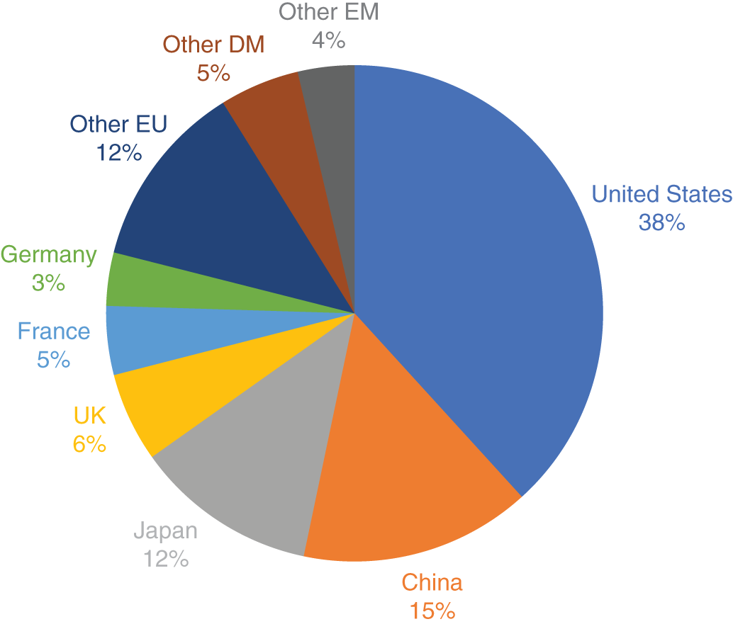
EXHIBIT 1.1 Market capitalization of global fixed income markets as of December 31, 2020. All securities are valued in USD. Fixed income securities are grouped into countries based on the domicile of the issuer and are dependent on source data availability at the country level.
Source: Data from Bank for International Settlements (www.bis.org/statistics).
The debt securities included in Exhibits 1.1 and 1.2 include domestic debt securities (DDSs) and international debt securities (IDSs). The Bank for International Settlements (BIS) defines DDS as those instruments issued in the local market of the country where the borrower resides, regardless of the currency in which the security is denominated, and IDSs as those instruments outside the local market of the country where the borrower resides. Approximately 80 (20) percent of fixed income securities are DDSs (IDSs) as of December 31, 2020. Correspondingly, our focus will be on domestic fixed income securities, as this reflects the bulk of the fixed income investment opportunity set. This is not to say that international securities are not relevant. They are, and in Chapter 7 we will discuss hard currency emerging market debt specifically. It is important to remember that although the issuance of debt securities by an issuer in multiple countries (and multiple currencies) does expand the investment opportunity set, these additional securities, while not totally redundant, are usually highly correlated with the domestic security.
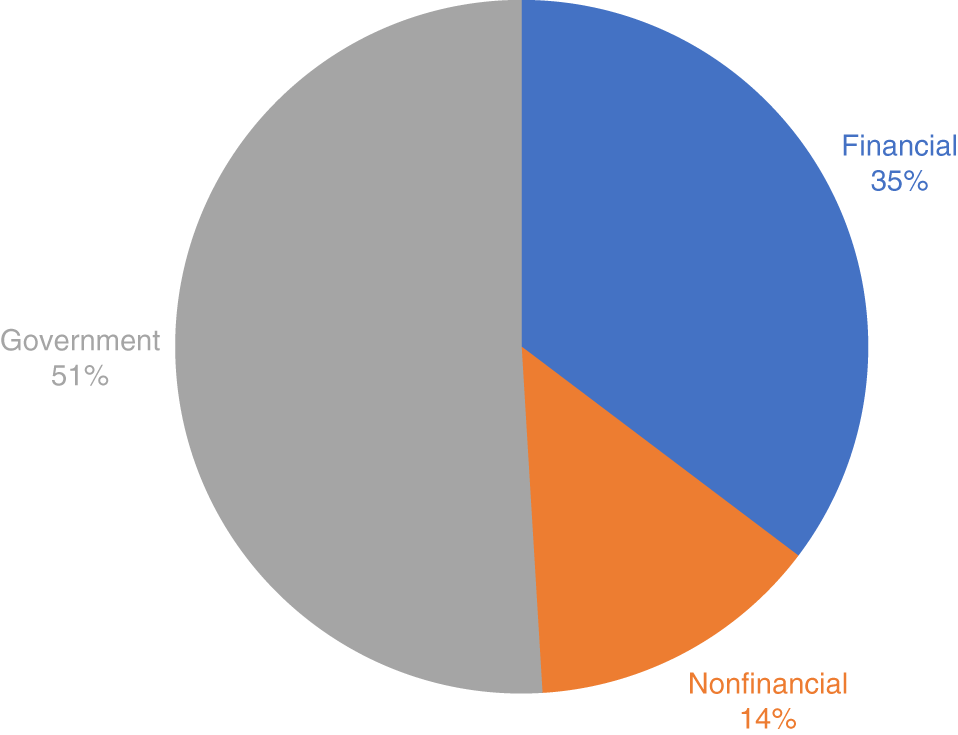
EXHIBIT 1.2 Market capitalization of global fixed income markets as of December 31, 2020. All securities are valued in US dollars. Fixed income securities are grouped into categories based on the nature of the issuing entity.
Source: Data from Bank for International Settlements (www.bis.org/statistics).
A final point to note about the size of the global fixed income market is that the BIS data is based on cash securities (i.e., bonds issued by governments and corporations). In addition to these cash securities, there is an extensive derivatives market covering fixed income. These include (i) interest rate derivatives (futures, options, and swaps) linked to the underlying cash bonds issued by governments (both developed and emerging markets), (ii) derivatives linked to specific securitized assets (e.g., the to be announced [TBA] market for mortgage pass‐through securities in the United States), (iii) single‐name credit derivatives (credit default swaps), and (iv) index‐level credit derivatives (e.g., Markit and iTraxx indices). These markets are also very large, and a key benefit of these derivative markets is the concentration of liquidity into specific issuers and specific issues for a given issuer (although a company typically has only common equity claim outstanding, it may have many bonds outstanding). As we will see in greater detail later in this book (especially Chapter 9 on liquidity), there is oftentimes difficulty in sourcing inventory for a specific fixed income security.
A driver of the limited liquidity in fixed income, especially relative to equity markets, is the breadth of securities to select from for a given issuer. For example, as of November 30, 2021, there were 1,744 bonds in the Global Treasury subindex within the Bloomberg Global Aggregate Index. Of these 1,744 bonds, 267 were issued by the United States and 554 were issued by what is collectively referred to as the G‐7 (excluding the United States): Japan (274), Italy (82), Germany (57), the UK (55), France (47), and Canada (39). There are many securities to choose from for each government issuer. A similar concentration in issuance is seen for corporate bonds where there are roughly seven bonds outstanding for each investment‐grade‐rated corporate issuer. As we'll see in detail in Chapters 5 (6) for government (corporate) fixed income securities, there is considerable redundancy across the multiple issues for a given issuer. Stated differently, bonds issued by the same issuer share a considerable amount of common variation. Investors are spoiled by breadth, and this leads to a bifurcation in liquidity across many redundant securities. Blackrock (2014) has noted the lack of standardization in the corporate bond market as a key driver of liquidity challenges. Although there are institutional reasons for the lack of standardization (e.g., issuance fees for intermediaries, cash flow maturity management from corporate treasury departments), there is limited need for so many securities from an investor perspective. A small number of securities (as few as two or three) can capture most of the return variation that is available to the investor. And this is where the derivative market can be very useful for the fixed income investor: liquidity can be concentrated in a small number of tenors for each issuer. Unfortunately, derivative markets are liquid for many but not all issuers and many but not all key tenors.
We can undertake a more detailed analysis of the investment opportunity set for fixed income investors by looking at the Bloomberg Global Aggregate Index. This is a very broad index commonly used as a policy benchmark by many large institutional asset owners. It contains investment‐grade‐rated bonds issued in multiple currencies that meet specific liquidity requirements (e.g., par value more than $300 million USD for USD‐denominated debt). As of December 31, 2020, the Global Aggregate Index included 26,514 individual bonds amounting to $67.5 trillion USD outstanding. Exhibit 1.3 shows the breakdown of the market capitalization of the Global Aggregate Index. The $67.5 trillion USD is broken down into (i) $35.9 trillion USD for Global Treasury (TSY) securities (includes all investment‐grade‐rated debt issued by developed market sovereign entities), (ii) $10.0 trillion USD issued by government‐related entities (GREL), (iii) $12.7 trillion USD issued by corporate (CORP) entities (includes all investment‐grade‐rated debt issued by corporations domiciled in developed markets), and (iv) $8.9 trillion USD of securitized (SEC) debt (the majority of which is mortgage‐backed securities from the main US government agencies).
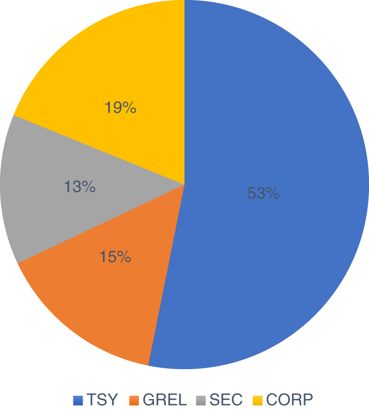
EXHIBIT 1.3 Market capitalization of Bloomberg Global Aggregate Index as of December 31, 2020.
Source: Data from Bloomberg Indices.
Exhibit 1.4 shows the breakdown of the number of issues contained within the Global Aggregate Index as at December 31, 2020. The 26,514 issues are comprised of (i) 1,681 bonds issued by developed sovereign entities, (ii) 5,828 bonds issued by government related entities, (iii) 13,831 bonds issued by corporate entities, and (iv) 5,174 bonds issued across agency and nonagency asset‐backed securities, commercial mortgage‐backed securities, and covered bonds. The proportional composition of the Global Aggregate Index looks very different when viewed through the lens of number of instruments; there are fewer government bonds outstanding, but they have a much larger market value per bond, and there are far more corporate bonds outstanding, but they have a much smaller market value per bond. The smaller issue size of corporate bonds is related to the liquidity challenges discussed earlier that we will return to in Chapter 9.
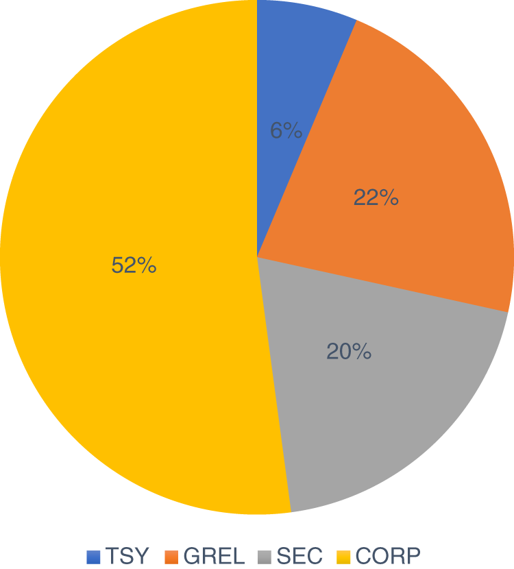
EXHIBIT 1.4 Composition of Bloomberg Global Aggregate Index as of December 31, 2020.
Source: Data from Bloomberg Indices.
1.3 WHAT DOES IT MEAN TO BE SYSTEMATIC?
We are talking about systematic active investing in fixed income markets. Now that we have a handle on fixed income markets, we need to agree on what it means to be systematic in your investment approach. This is challenging. A systematic investor cannot be defined as an investor who has a quantitative approach. After all, as we will see later in this chapter, all investors in fixed income markets need to be able to understand (if not compute) derivatives (I mean duration and convexity, which we will cover in detail later in this chapter), which would seem to qualify most fixed income investors as quantitatively able. So, what then distinguishes a systematic investor? And if you are not a systematic investor, then what are you? These are related questions, and to help answer these questions I will make use of a simple visual (Exhibit 1.5) that is adapted from an AQR Alternative Thinking (2017) publication titled “Systematic vs Discretionary.”
Exhibit 1.5 identifies both differences and similarities between systematic and discretionary approaches. While it can be natural to think of investment approaches as mutually exclusive, this would be a disservice to both approaches. So, let's first emphasize what is, and must be, common across the investment approaches. Both systematic and discretionary investors are active investors. That means they are both willing to entertain that the market is not completely efficient with respect to certain value‐relevant information, and that they have the investment acumen to identify that information and trade upon it profitably. It may also mean that they believe that markets are efficient but that there are opportunities to provide liquidity to the market to take advantage of price‐taker traders (e.g., avoiding bad selling practices from rating downgrades or other index exclusions, and/or actively seeking out new issue concessions).
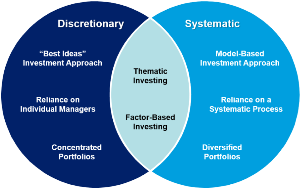
EXHIBIT 1.5 A comparison of systematic and discretionary investment approaches.
Source: Data from AQR (2017). Systematic vs Discretionary. Alternative Thinking Quarterly, Q3 2017.
Both systematic and discretionary active investors must have a sound understanding of the sources of returns and risks within the fixed income market. Again, almost by definition, systematic and discretionary investors must share some common beliefs about the determinants of fixed income security returns. Indeed, I have often been told over the years that what we say and do, as systematic fixed investors, at a high level, sounds very familiar to a discretionary investment approach. A few years ago, I gave a presentation in front of a large internal team of fixed investment professionals at a large sovereign wealth fund, and I followed a senior investment professional from a large traditional (discretionary) fixed income asset manager. The head of the internal fixed income team spoke to me after the event and commented, “You sound very similar to the traditional (discretionary) manager, yet your final portfolios are quite different.” It is that difference that this book seeks to identify and promote the diversifying potential of. A good systematic process should be trying to capture the best bits of a fundamentally driven discretionary approach and apply that in a highly diversified manner.
As we will see in Chapter 2, understanding risk‐free yields and spreads is at the heart of fixed income investing. This is true for both the systematic and discretionary investor. A systematic investor does not have access to a secret sauce allowing them privileged access to the data‐generating process that gives rise to asset returns. If only that were true! This book will lay out a fundamental framework to understand the risks and returns for the most common fixed income securities. Both discretionary and systematic fixed investors are likely to share common beliefs on this fundamental framework. The intersection of the Venn diagram in Exhibit 1.5 is a nod to this similarity in core investment beliefs, noting that the Venn diagram is not drawn to scale (if it were, the common area would be much larger, as I think the investment approaches are more similar to each other than they are different).
So, what then is the difference between systematic and discretionary investment approaches? I believe the primary differences are the reliance on individuals (discretionary) rather than a repeatable process (systematic), and the reliance on an investment narrative/story (discretionary), rather than an investment model (systematic). These differences may sound superficial at first glance, but they are what distinguishes a systematic process from a discretionary approach. The “narrative” in a systematic investment process is a set of measurable characteristics capturing fixed income assets that have the potential to generate higher excess returns. For fixed income this will include measures of value, quality, carry, and momentum (and other measures). These characteristics will be measured across a wide set of fixed income securities (the hundreds of government bonds and thousands of corporate bonds discussed earlier in this chapter). The “narrative” in a discretionary investment process will typically reflect a combination of top‐down macro views (on inflation, growth, etc.) and detailed bottom‐up credit analysis on specific issuers. The implicit belief is that this deeper contextual analysis is the source of investment value add. Both approaches have their merits (breadth for systematic and depth for discretionary).
The systematic approach does not rely on any one individual on a day‐to‐day basis to make trading decisions. Trade lists are generated as the result of a systematic process. That is not to say individuals do not look at the trade list. They do, just that the role of the individual is to confirm the integrity of the data and ensure that there are not any unmodeled news or risks that would negate the purpose of the intended trade (e.g., your systematically generated buy list includes a bond from a corporate issuer for which overnight, there was news of a leveraged buyout or some other corporate action). In those cases, there is a clear role for human intervention to take risk off the table in a controlled manner. Indeed, these interventions can also be built in a somewhat systematic manner. In contrast, the discretionary approach leans heavily and regularly on the lead portfolio manager. That individual is the holder of investment decision rights, and their narrative is inherently less objective than a prespecified systematic process. That approach has the potential benefit of responsiveness to changing market conditions and changing drivers of fixed income returns. However, it comes with the risk of individual biases that may be the root source of investment opportunities to start with. The investment approaches are different in their implementation of what I think are reasonably similar core investment beliefs/narratives.
The final portfolios are very different in expected ways. A more diversified portfolio typically means (i) more line items in the final portfolio (this characteristic is common for systematic portfolios), and (ii) lower tracking error as a direct consequence of the more diversified portfolio. This does mean that a discretionary fixed manager has the potential to generate higher excess returns, but that comes with additional risk. What ultimately matters for asset owners is the excess return generated per unit of active risk (a ratio of return to risk is called a Sharpe ratio or an information ratio, depending on the return that is examined: excess of cash returns is a Sharpe ratio, and excess of beta/benchmark returns is an information ratio). There is minimal evidence to suggest the information ratios are different across systematic or discretionary managers (for equity markets, AQR 2017, note that while the excess of benchmark returns are similar for systematic and discretionary managers, discretionary managers have a higher tracking error leading to slightly lower information ratios). We will discuss the Sharpe ratios and information ratios of incumbent active fixed income managers in detail in Chapter 4.
It is also important to remember that not all systematic fixed income managers will be the same. Just as not all discretionary managers are expected to hold similar portfolios, there is no reason that all systematic managers will hold the same portfolio. Indeed, research in equity markets has shown that the average pairwise correlation between excess returns for systematic active equity managers is as low as the average pairwise correlation between excess returns for discretionary active equity managers (see e.g., Lakonishok and Swaminathan 2010, and AQR 2017). As we work through the systematic fixed income framework developed in this book, hopefully the breadth of choices that must be made to build a final portfolio will become clear. Variations in those choices across asset managers will lead to meaningful differences in portfolio outcomes. At the end of the day, what matters most to an asset owner is a well‐implemented (read liquidity and risk aware) portfolio that targets exposure to your investment hypothesis (read narrative for the discretionary manager or investment model for the systematic manager). It is those signals and implementation details that we will cover in detail in later chapters.
A word of caution is useful for the term discretionary. In a pure sense, all active investors are discretionary. A systematic investment approach requires many decisions to be made from everything to selecting data vendors to signal construction, signal weighting choices, various liquidity, and risk management choices, and so forth. All these decisions are discretionary in that a human (or group of humans) must make them. What is different is the stage of the investment process at which those decisions are made. A systematic investor is trying to make discretionary decisions at the start of the investment process. Think of these as strategic decisions that are then codified into a repeatable and scalable investment process.
A recipe for a systematic investment approach might look like the list that follows. I first heard this described when working at Barclays Global Investors (Richard Grinold was a key proponent) and I used this framework to summarize a broad literature on accounting‐based anomalies in the equity market back in 2010 (see Richardson, Tuna, and Wysocki 2010):
- Credible hypothesis: Does your investment idea pass a “sniff test”? What is it about your idea that would lead to future excess returns? Why does the market price not already reflect this information? What informational inefficiency or liquidity provision are you targeting? This is a subjective conceptual discussion. To the extent that there is discretion in the systematic investment process, this is the stage where it is most important.
- Robust predictive power: Take your investment idea to the data and assess whether it robustly predicts future returns. This empirical exercise should look for as many possible markets to test the idea (developed and emerging markets, different time periods, other related asset classes, etc.).
- Test the mechanism: Flesh out the implications of the investment hypothesis. If your measure is related to mispricing, then look for evidence beyond simple return correlations. If the investment idea is attributable to market participants failing to fully utilize information that is useful for forecasting fundamentals (e.g., inflation or growth for government bonds or free cash flows for corporate bonds) then test whether your “signal” can forecast future fundamentals in addition to future returns. Go one step further and assess whether capital market participants who are in the business of forecasting these fundamentals make systematic forecasting errors with respect to your information. These non‐return‐based tests add substantial conviction to the efficacy of your investment idea. In‐sample fitting of returns (data mining) is a serious risk. Although many have criticized the lack of out‐of‐sample results in finance and advocate for multiple‐testing adjusted test statistics, a simple protection for this risk is robust testing of the underlying economic mechanism.
- Implementation: Test whether your investment idea survives the various implementation challenges. This would include expected transaction costs, potential market impact, inability to source inventory at time of trade, risk‐based position limits, and so forth. Many ideas that look good on paper are too costly to implement in practice.
- Additivity: Is your investment idea additive to what is already in the portfolio? Although there is a path dependency here to be handled (i.e., the first signal would seem to get a free pass by this criteria) this is critically important, as what matters is the active risk and return at the final portfolio level. If you keep adding highly correlated signals, you will end up with a very unbalanced portfolio.
There are clearly some necessary ingredients for a systematic investment approach to be adopted. Most notable is the need for reliable data. All the aforementioned testing procedures require data. That data needs to exist and needs to be point‐in‐time (i.e., available historically at the same time that market participants had access to it) and of reliable quality, so any hypothetical portfolio (back‐test) is at least partially informative of what you may expect to experience in the future. One other key aspect for the success of systematic investing is liquidity in the markets in which the assets trade (both primary and secondary markets). There are fixed income markets (e.g., municipal bond markets and cash mortgage‐backed securities) that are inherently ill suited for standard systematic investment processes. There is little point building an investment infrastructure to generate trade lists for assets that do not trade after issuance or that trade very infrequently. Trading as a liquidity taker in fixed income markets can be very costly, especially relative to the excess return potential, so liquidity in the market is almost a necessary condition to utilize a systematic investment approach. We will discuss the importance of liquidity provision for the successful implantation of systematic fixed income portfolios in Chapter 9.
How common are systematic investment approaches within the fixed income asset class? It is very difficult, if not impossible, to answer this question precisely. We can look at regular databases that store information about investment vehicles. Exhibit 1.6 shows the size and breakdown of institutional systematic fixed income investment vehicles as at December 31, 2020. To construct this chart various choices are made. Investment vehicles are long‐only and fixed income benchmarked and the definition of systematic is made subjectively based on an understanding of which asset managers have described themselves as having a systematic approach to their investment philosophy. Using this subjective criteria and fund data from eVestment, the total size of the systematic fixed income investing universe is about $120 billion USD. That is tiny relative to the size of the overall fixed income universe. But this total has grown significantly over recent years, adding more than $50 billion in the past five years. Exhibit 1.6 obviously misses a considerable portion of actively managed systematic fixed income assets. For example, there could be internal pools of capital run systematically by asset owners, and there could be internal systematic tools used to complement traditional discretionary approaches. However, even including conservative estimates for the potential additional systematic fixed income approaches, systematic approaches are in the minority. Exhibit 1.6 notes that corporate strategies (both investment‐grade and high‐yield) account for roughly half of systematic fixed income assets and government bond or aggregate index mandates account for the rest. As we will see throughout this book, government and corporate bonds are the two areas in which a systematic approach is most likely to succeed: there is sufficient data access and market liquidity.
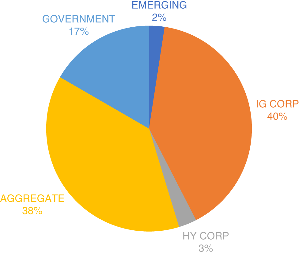
EXHIBIT 1.6 The size of the systematic fixed income investing universe.
Source: Data from eVestment.
What does the small size of actively managed systematic fixed income funds mean? I am a firm believer in the notion of equilibrium. The fact that something does not exist, or exists only at small scale, may speak to the inefficiency of that practice. That is certainly a possible interpretation of the small scale of active systematic fixed income investing. However, there is another, more optimistic interpretation. It is difficult to successfully implement a systematic approach in fixed income, and it is challenging to convince asset owners of the efficacy of this alternative investment approach. I am a firm believer in this optimistic interpretation. Indeed, one can view this book as a continued attempt to beat the drum of the legitimacy of systematic fixed income investing. This is a challenge to be embraced by asset managers and asset owners alike. Asset managers, and to some extent asset owners assessing whether, and how, to develop internal systematic capabilities, need to overcome inertia and cultural frictions. There is natural skepticism of new approaches, and incumbents are naturally averse to new things that threaten their existence. Of course, just because something is new does not mean it is better. Fixed income, and especially credit sensitive assets like corporate bonds, face considerable liquidity challenges and security idiosyncrasies that may make it too difficult to be successful as a systematic investor. So, a healthy dose of self‐doubt is necessary, and we will cover these data and liquidity challenges in detail in Chapters 6 and 9. But, this introspection on investment challenges should be applied uniformly across all active fixed income investors. After all, concerns about liquidity, the ability to trade into and out of assets, and confidence in your ability to measure expected returns for idiosyncratic assets are ultimately a data challenge. And data is central to any investment process, whether it is systematic or discretionary.
1.4 WHICH FIXED INCOME MARKETS WILL THIS BOOK FOCUS ON?
The focus in this book will be on what I call public fixed income markets. This means constituents of the regular parent indices that most large asset owners use for their fixed income allocations. Versions of the Aggregate Index (Global, US, or European) will capture the breadth of investment‐grade‐rated fixed income assets that we will focus on. Section 1.2 of this chapter laid out the key components of the Global Aggregate Index, and our focus will be on the government and corporate sectors.
In addition, we will look at emerging market debt in Chapter 7. Our focus there will be mostly on hard currency (USD) debt issued by sovereign and quasi‐sovereign entities. We will discuss the huge growth in local currency emerging market debt, but the return drivers of emerging government local currency debt is similar to that of developed government local currency debt, so we will focus our discussion of local currency debt on the differences across developed and emerging markets. We will have little to say about emerging market corporate debt, because the data quality and market liquidity is limited in this market, and consistent with the discussion in Section 1.3, a systematic approach in the emerging market corporate space is more challenging from an operational perspective.
High‐yield corporate bonds are also important to cover. The distinction between investment‐grade (IG) and high‐yield (HY) rated corporate issuers is somewhat arbitrary. The returns data generating process for IG‐rated corporate issuers is more similar than dissimilar to HY‐rated corporate issuers. In Chapter 6, when we talk about investment frameworks for credit sensitive assets, we will emphasize the similarities across IG and HY corporates, and, where necessary, we note differences in return drivers. Similarly, in Chapter 9 when we discuss trading and liquidity considerations for fixed income securities, we will discuss trading differences in primary and secondary markets for IG‐ and HY‐rated corporate bonds (for both North America and Europe) and the unique challenges and opportunities that liquidity provision creates for a systematic investor.
The leveraged loan market we will not cover in detail in this book. Leveraged loans are a type of syndicated loan issued by corporations that are high‐yield‐rated (often as part of corporate merger activity or buyout financing). These loans trade on secondary markets with extended settlement terms that make them less suitable for any investment vehicle that has frequent dealing. The leverage loan market is about $1.6 trillion USD as at December 31, 2020.2 The return drivers of loans are similar to that of corporate bonds, so it is not any lack of understanding of return drivers that makes loans less suitable for a systematic investment process. It is a combination of extended settlement, limited secondary market liquidity, and challenges in sourcing reliable data for the private companies that issue loans that makes it challenging for systematic approaches to be used in the leveraged loan market. But these challenges also create opportunities as it less likely to be a crowded area.
Finally, this book will have little to say about the growing private debt markets. Global private debt markets have grown from essentially nothing in the early 2000s to nearly $1 trillion USD as of December 31, 2020 (see, e.g., JP Morgan 2021) covering mezzanine financing, direct lending, and distressed/special situations. Again, there is nothing structural about the return generating process of private markets that makes a systematic investment approach unsuitable. It is the data and operational challenges that make it difficult. Private markets are notorious for a lack of secondary market liquidity, and in the case of private debt it can be very difficult to source data that can be used in a consistent and reliable way across investment opportunities. As with leveraged loans, these challenges also present opportunities for those with data and liquidity access.
1.5 COMMONLY USED FIXED INCOME ANALYTICS
As discussed at the start of this chapter, fixed income security valuation focuses on the denominator. Let us work with a simple example to illustrate some of the key concepts related to the language of fixed income security pricing. We will work with a simple $100 par value 10‐year maturity coupon bearing sovereign bond. The bond pays 2 percent annual coupon every six months (so effectively 1 percent compounded every six months). It is issued on January 1, 2022. Exhibit 1.7 illustrates the cash flow profile of this bond. We can write the price at time of issue for this bond as follows:
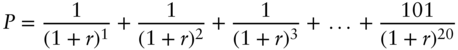
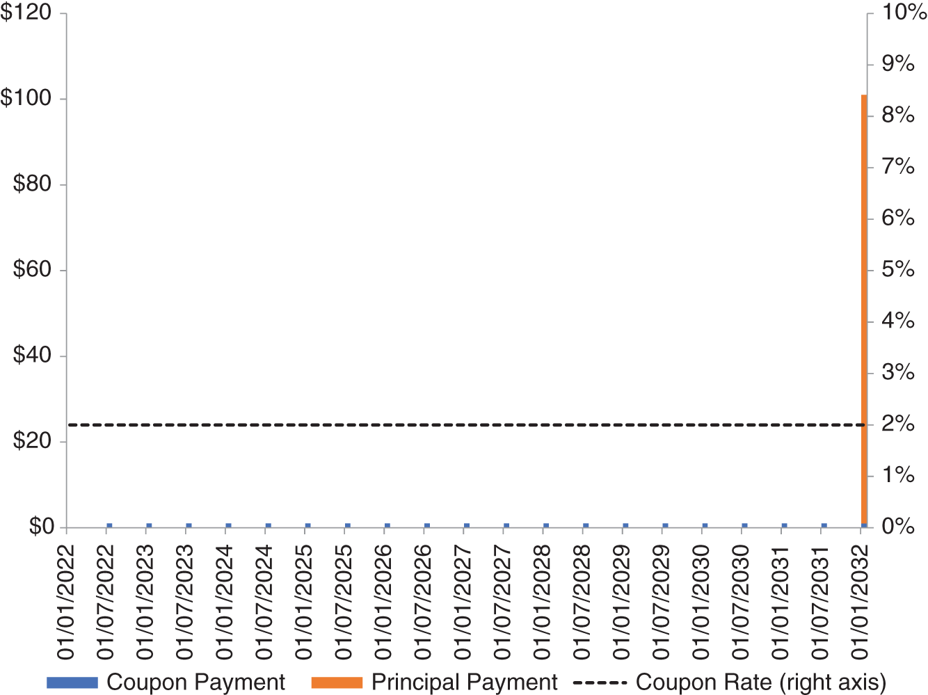
EXHIBIT 1.7 Cash flow profile of a $100 10‐year coupon bond issued on January 1, 2022, with a 2 percent coupon rate paid semi‐annually.
There is an inverse relation between price and discount rate, r. This is a highly nonlinear equation and captures the key element of fixed income investing: what is your view on r? Even working with an assumed flat term structure of discount rates (which we will loosen in Chapter 2 and beyond) it is easy to see that the impact of a change in r on price (P) will depend critically on the maturity profile of the cash flows.
Fixed income market participants tend to use the label yield to describe the discount rate for valuing fixed income securities. The prevailing yield can be thought of as an indicator of the expected return for a given fixed income security. It tells you the return an investor will receive for buying and holding the fixed income security to maturity, assuming no capital losses from forced selling or default prior to maturity and assuming the yield is the also the reinvestment rate for any coupons. So, what do yields look like for standard fixed income securities? Exhibit 1.8 shows the yield to worst (this is simply a measure of yield to maturity that adjusts for any embedded optionality or other contractual features that shortens the expected life of the fixed income security) for the Bloomberg Global Aggregate Index (bold line) as well as the four primary subindices (TSY, GREL, SEC, and CORP) over the 2001–2020 period.
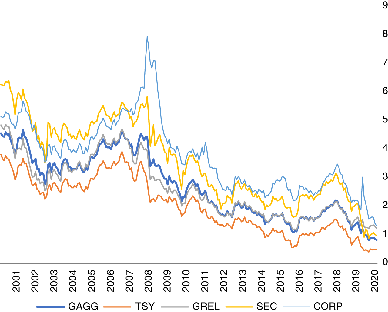
EXHIBIT 1.8 Yield to worst of Bloomberg Global Aggregate Index and subindices over the 20‐year period ending December 31, 2020.
Source: Data from Bloomberg Indices.
There is a clear downward trend in yields, especially over the past decade. This downward trend is global in nature and yields are now at some of the lowest levels ever. That is a strong statement to make, but as can be seen in Exhibit 1.9, yields on government bonds today are at the lowest levels they have ever been (going back to the 1300s). The data for this exhibit comes from the Global Financial Database, and I have selected representative bonds through time as a proxy for the center of global financial markets. Over the past 700 years, the financial center of the world has passed from Italy to the Netherlands to England to the United States. Data includes the Consolidated Bonds of Genoa from 1304 to 1408, the Prestiti of Venice from 1408 to 1500, the Juros of Spain from 1504 to 1519, the Juros of Italy from 1520 to 1598, government bonds of the Netherlands from 1606 to 1699, English bonds, primarily the British Consol from 1700 to 1918 and United States 10‐year Treasury bonds from 1918 to 2020. The most notable aspect of Exhibit 1.9 is the sharp decline in government bond yields over the most recent period. When market observers say interest rates are low, they aren't wrong! Of course, the data quality back in time, and any strict comparability through time, is questionable, but the pattern of historically low yields today is undeniable. Indeed, as at December 31, 2020, some 4,251 bonds out of the 26,514 bonds included in the Bloomberg Global Aggregate Index traded at negative yields. Collectively these bonds accounted for $16.1 trillion USD out of the total $67.5 trillion USD market capitalization of the entire index. These bonds were issued by sovereigns (mostly) and corporates around the world (Japan, Germany, and France accounted for 30, 15, and 15 percent, respectively). Low, and negative, yields are a topic we will discuss in Chapters 2 and 3 about the strategic and tactical case for allocating to fixed income securities.
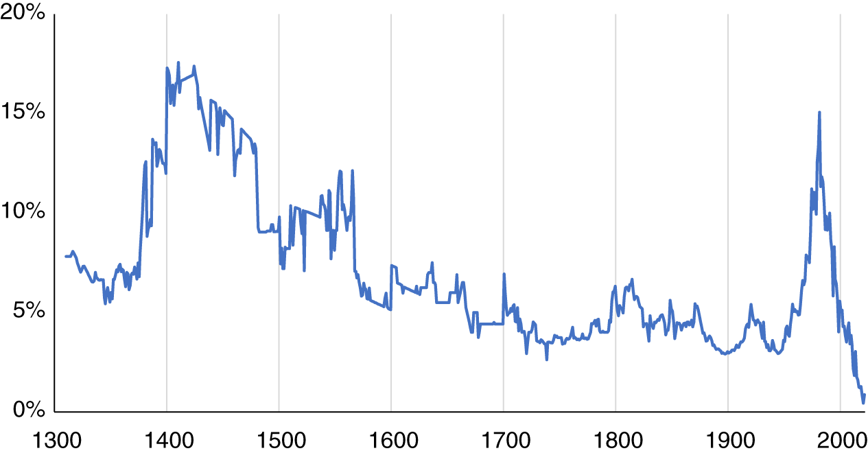
EXHIBIT 1.9 Proxy government bond yields from 1304 to 2020.
Source: Global Financial Database (https://globalfinancialdata.com/7-centuries-of-government-bond-yields).
The concept of duration formalizes the relation between changes in prices and discount rates by taking the first‐order derivative of Equation 1.2. Mathematically this can be written as ![]() . This simply means how does the price of the bond change when there is a change in the discount rate. The negative sign is convention: even though the relation between prices and discount rates is negative duration is typically quoted in positive units. The second multiplication,
. This simply means how does the price of the bond change when there is a change in the discount rate. The negative sign is convention: even though the relation between prices and discount rates is negative duration is typically quoted in positive units. The second multiplication, ![]() , often causes confusion when you first see duration written mathematically. It just means that duration is measured for a bond at a given price (i.e., a given starting yield). The same set of cash flows will have a different duration depending on the starting yield. We will return to this point later in this chapter.
, often causes confusion when you first see duration written mathematically. It just means that duration is measured for a bond at a given price (i.e., a given starting yield). The same set of cash flows will have a different duration depending on the starting yield. We will return to this point later in this chapter.
An equivalent way to capture the intuition of duration is a dollar weighting of the cash flows over the life of the fixed income security. All else equal, bonds with a longer time to maturity – and hence the more the cash flows are further into the future – have higher duration. This intuition is very powerful to quickly understand other deterministic differences in duration based on bond characteristics. Bonds with a higher coupon rate have a shorter duration (holding maturity fixed). Conversely, bonds with low coupons have a longer duration. There is a limit for the value of duration: a zero‐coupon bond has a duration equal to its maturity.
Duration is a powerful summary statistic used to describe the properties of fixed income securities. It is worthwhile to understand exactly why. Duration can be close to a sufficient statistic for describing the first‐order impact of changes in yields (interest rates) on prices of fixed income assets. Let us continue with our example of a 10‐year coupon bond from earlier in this chapter. We can compute the duration of this bond when issued at par as 9.16 years. This duration of 9.16 means that for a 1 percent change in yields (discount rates) the price of the bond would change by 9.16 percent (or $9.16 if this change in yields was observed in the year after issuance at par). This implied change in price is, however, an approximation. While it is very useful for small changes in yields, duration's efficacy as a summary measure of interest rate sensitivity is lessened for bonds that exhibit greater convexity. Oh dear, we have another term to grapple with.
Convexity is another commonly used analytic to describe the sensitivity of fixed income security prices to interest rates. Mathematically, it can be written as ![]() . This is simply the second‐order derivative reflecting how prices change for a given change in yields (discount rates). Duration was the first‐order derivative, so you can think of convexity as the first‐order derivative of how duration changes for a given a change in yields. This is perhaps easiest visualized. Exhibit 1.10 shows the relation between price and yield for our 10‐year bond. The solid black line computes the precise value of our bond's cash flows for yield levels that vary from between 0 and 4 percent. The solid black point corresponds to a price of 100 and yield of 2 percent consistent with a 2 percent coupon bond issued at par. Using duration of 9.16 years we can approximate the value of our bond for all yield values between 0 to 4 percent. To do this we simply compute the price of the bond as the starting price ($100) plus the change in yield multiplied by –1 times duration (9.16). This is shown as the solid gray line in Exhibit 1.10. It should be readily clear that this is also a point of tangency on the curve capturing the relation between price and yield (this is exactly what a first derivative captures). It is also clear that for small changes in yields the distance between the solid gray line and the solid black line are quite small. This is generally true for all fixed income securities. The quality of the approximation is lower for large changes in yields and for fixed income securities with greater convexity. We can easily repeat our approximation using knowledge of both duration and convexity. This is shown on Exhibit 1.10 as the dashed gray line and the approximation error is now very small across all possible values for yield. Again, this should not be surprising as that is exactly what a second derivative (convexity) is capturing. Convexity is not going to be the focus of this book as we will be considering primarily government bonds and corporate bonds that generally do not have substantial curvature in their relation between prices and yields.
. This is simply the second‐order derivative reflecting how prices change for a given change in yields (discount rates). Duration was the first‐order derivative, so you can think of convexity as the first‐order derivative of how duration changes for a given a change in yields. This is perhaps easiest visualized. Exhibit 1.10 shows the relation between price and yield for our 10‐year bond. The solid black line computes the precise value of our bond's cash flows for yield levels that vary from between 0 and 4 percent. The solid black point corresponds to a price of 100 and yield of 2 percent consistent with a 2 percent coupon bond issued at par. Using duration of 9.16 years we can approximate the value of our bond for all yield values between 0 to 4 percent. To do this we simply compute the price of the bond as the starting price ($100) plus the change in yield multiplied by –1 times duration (9.16). This is shown as the solid gray line in Exhibit 1.10. It should be readily clear that this is also a point of tangency on the curve capturing the relation between price and yield (this is exactly what a first derivative captures). It is also clear that for small changes in yields the distance between the solid gray line and the solid black line are quite small. This is generally true for all fixed income securities. The quality of the approximation is lower for large changes in yields and for fixed income securities with greater convexity. We can easily repeat our approximation using knowledge of both duration and convexity. This is shown on Exhibit 1.10 as the dashed gray line and the approximation error is now very small across all possible values for yield. Again, this should not be surprising as that is exactly what a second derivative (convexity) is capturing. Convexity is not going to be the focus of this book as we will be considering primarily government bonds and corporate bonds that generally do not have substantial curvature in their relation between prices and yields.
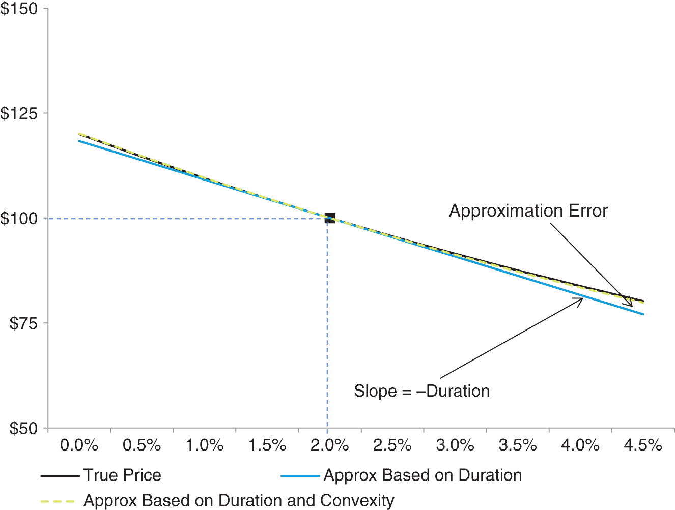
EXHIBIT 1.10 Relation between price and yield for a $100 10‐year coupon bond issued on January 1, 2022, with a 2 percent coupon rate paid semi‐annually. The solid black line reflects the actual price at all yield levels between 0 and 4 percent. The solid blue line reflects the approximation using duration alone. The dashed green line reflects the approximation using duration and convexity.
We are now sufficiently well armed (and dangerous) to continue our exploration into fixed income investing. Before we go further, it is useful to be aware of the multiple ways in which duration measures are utilized. Fixed income securities embody at least two sources of risk: (i) time value of money considerations inclusive of refinancing/rollover risks, and (ii) spread risk reflecting the possibility that your contractually specified cash flows may not materialize (you may get paid sooner or later than you expected, or in some cases not at all). We can therefore generalize our fixed income pricing equation as follows:

We have now decomposed the discount rate to have two components: (i) y, reflecting the yield for a riskless security, and (ii) s, reflecting a spread for the additional risks of nonpayment. Equation (1.3) assumes no term structure associated with either yields or spreads. Our duration measures can therefore be either, ![]() , or,
, or, ![]() . The first measure is typically called effective (modified) duration and captures the change in risk‐free interest rates (yields) on fixed income prices. The second measure is typically called spread duration and captures the change in (credit) spreads on fixed income prices. Both are partial derivatives that consider how changes in y or s affect price independent of how the change in y or s may affect each other. To further complicate matters, there is a term structure for both y and s. Thus, there can be a multitude of duration measures (reflecting risk‐free discount rates or spreads at different maturity points). We never said fixed income investing would be easy! But it is useful to note that for many of the government and corporate bonds that we examine in this book, we can go a long way in understanding return variation by utilizing a single yield or spread sensitivity.
. The first measure is typically called effective (modified) duration and captures the change in risk‐free interest rates (yields) on fixed income prices. The second measure is typically called spread duration and captures the change in (credit) spreads on fixed income prices. Both are partial derivatives that consider how changes in y or s affect price independent of how the change in y or s may affect each other. To further complicate matters, there is a term structure for both y and s. Thus, there can be a multitude of duration measures (reflecting risk‐free discount rates or spreads at different maturity points). We never said fixed income investing would be easy! But it is useful to note that for many of the government and corporate bonds that we examine in this book, we can go a long way in understanding return variation by utilizing a single yield or spread sensitivity.
Now that we have a basic understanding of duration it is useful to consider how duration has changed over time for the broad fixed income markets. Exhibit 1.11 shows the maturity profile of the Bloomberg Global Aggregate Index (bold line) as well as the four primary subindices (TSY, GREL, SEC, and CORP) over the 2001–2020 period. Except for securitized assets, there has been a consistent trend of longer dated bond issuance. This is partly attributable to the prevailing lower interest rates over the past decade. Combining that longer dated issuance with lower yields there is an even greater effect on duration (all else equal, lower yields imply a more negative relation between price and yield, and hence longer duration). Indeed, we see that clearly in Exhibit 1.12.
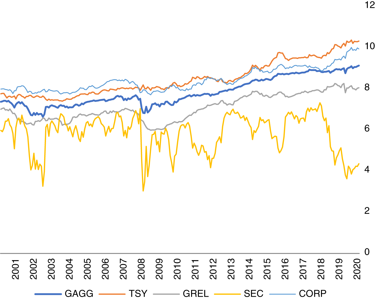
EXHIBIT 1.11 Maturity profile of Bloomberg Global Aggregate Index and subindices over the 20‐year period ending December 31, 2020.
Source: Data from Bloomberg Indices.
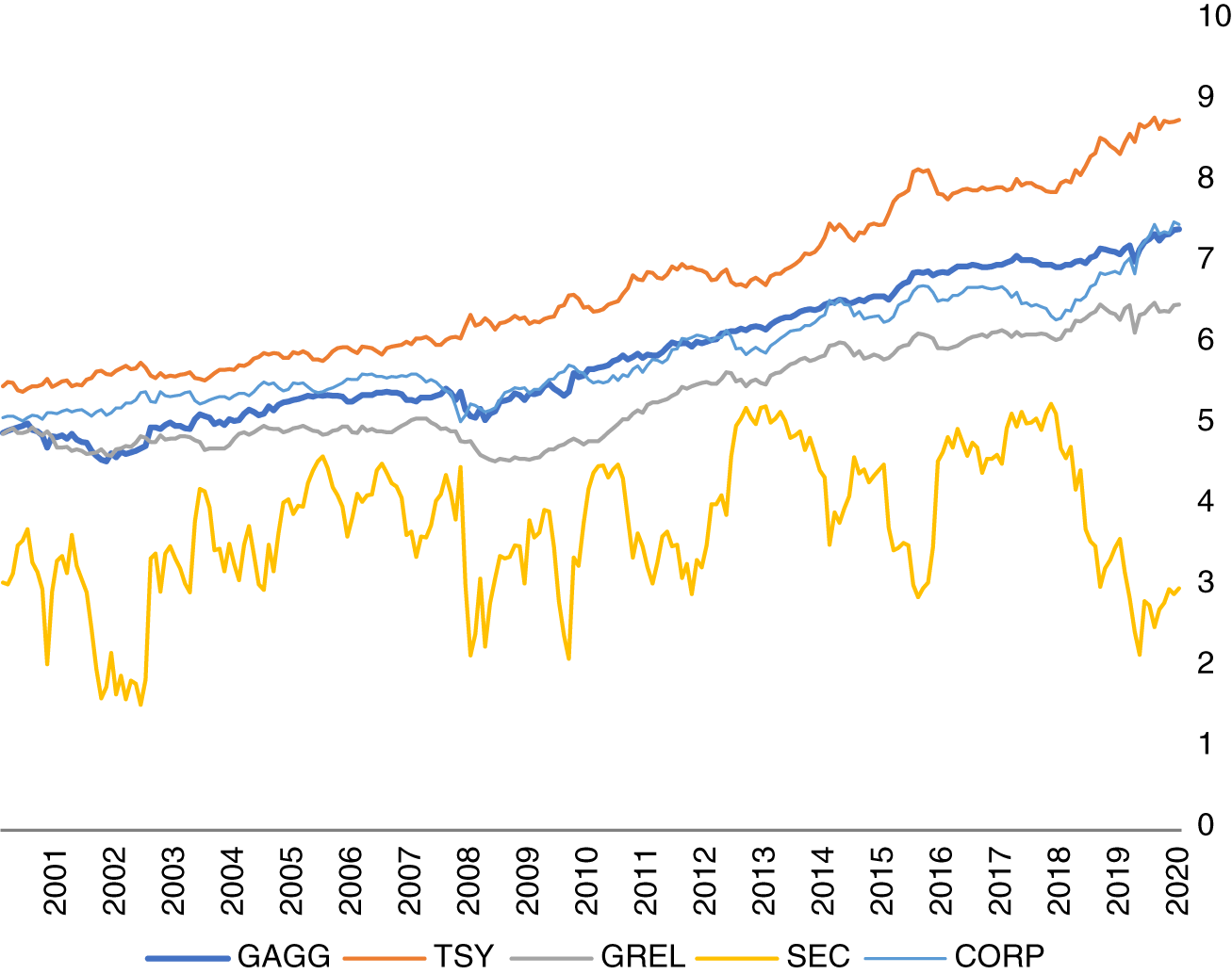
EXHIBIT 1.12 Duration profile of Bloomberg Global Aggregate Index and subindices over the 20‐year period ending December 31, 2020.
Source: Data from Bloomberg Indices.
This evolution of the duration profile of fixed income securities is very important for asset owners. All else equal, any change in interest rates will have a greater effect on the prices of fixed income securities. In the current low yield environment, there is heightened concern about the prospect of rising interest rates and the impact of expected interest rate rises on longer‐term yields and hence fixed income prices. Before rushing to any tactical asset allocations decisions at this point, Exhibit 1.12 is simply a cautionary reminder of how small changes in interest rates may have an outsized impact on the value of our fixed income allocation. In Chapter 2 we will discuss determinants of long‐term yields, and we will then be in a better position to make strategic and tactical recommendations for the fixed income asset class.
1.6 OTHER FIXED INCOME CONSIDERATIONS
We have a few more ancillary topics to cover before we can move into the details of systematic fixed income investing.
1.6.1 Currency and Hedging
Most fixed income indices include bonds that are issued in multiple currencies. This can be due to an issuer opting to issue multiple bonds in different currencies or to the global nature of the index that includes issuers domiciled in different countries, who issue bonds in their local currencies. As with equity investment decisions, the asset owner needs to decide if they want the additional volatility of currency movements in their fixed income portfolio. The decision for fixed income investors is even more important, as the relative volatility of currency movements can dominate the volatility of the underlying fixed income asset. The perspective of this book is to operate with currency hedging in place. This ensures that active risk‐taking decisions of fixed income securities are driven by investment views of the issuer and the specific issue without regard for the currency in which the bond is issued. A key benefit of this approach is delineating returns sources and allowing for specific investment views on (i) interest rates for country A relative to country B, and (ii) currency of country A relative to currency of country B. If you work with unhedged returns you are combining those views together and you are forced to have common views across the interest rate and currency portion of the fixed income security. It is better to separate them, and then you can take active currency views using currency forward contracts.
1.6.2 Home Bias
Over the years of managing fixed income portfolios, the extent of home bias in strategic fixed income allocations from asset owners I always found puzzling. Although asset owners make small allocations to emerging market debt and high‐yield corporate debt from outside their local area, as a general rule, they have core fixed income policy benchmarks tied to their local geographies. For example, asset owners based in Australia will benchmark their core fixed income holdings to the Australian version of the Aggregate Index. Similar patterns are observed for North American‐ and European‐based asset owners who benchmark their core fixed income holdings to the European and US versions of the Aggregate Index, respectively.
Exhibits 1.13 and 1.14 show this striking home bias. Using data from eVestment, the charts show the breakdown in the domicile of fund assets for two broad categories of core fixed income funds. First, in Exhibit 1.13 I show the breakdown in the approximately $1.9 trillion USD managed by nearly 300 individual funds benchmarked to the US Aggregate Index. Fully 96 percent of these funds are domiciled in the United States. Examination of the Core Plus category also reveals a similar extent of home bias (96 percent of Core Plus funds are also domiciled in the United States). Home bias is pervasive. In contrast, of the roughly $400 billion USD managed by slightly more than 100 funds benchmarked to the Global Aggregate Index, we see a far more diversified set of funds domicile. Global fixed income allocations are also less common.
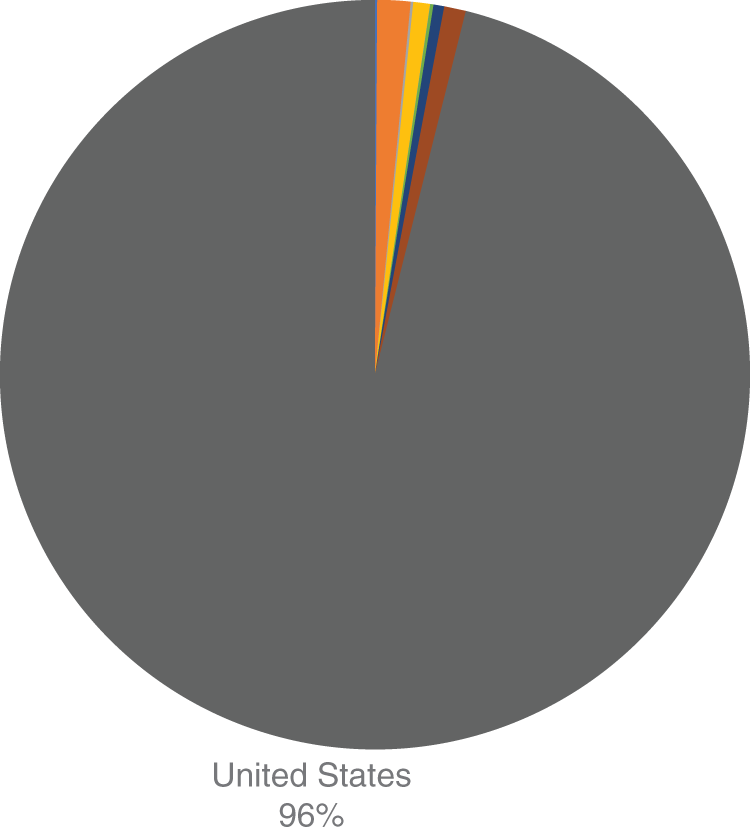
EXHIBIT 1.13 Domicile breakdown of institutional funds benchmarked to the US Aggregate Index.
Source: Data from eVestment.

EXHIBIT 1.14 Domicile breakdown of institutional funds benchmarked to the Global Aggregate Index.
Source: Data from eVestment.
There can be legitimate reasons for home bias. Core fixed income allocations are often an explicit liability hedge or economic hedge. In the case of a liability hedge, the cash flow profile inclusive of currency may be the preferred path. In that case, home bias is consistent with achieving that asset‐liability match. If the purpose of the core fixed income allocation is an economic hedge, then ensuring the asset side of the asset owner's portfolio faces similar economic risks, thus it may also be optimal to exhibit some degree of home bias. What surprises me is the extent of the home bias. You see this in the data and across hundreds of client meetings over the years.
The key consideration for asset owners here is the potential loss of international diversification. It is true that the benefit of international diversification has waned over time as the financial system has become more interconnected (international supply chains connecting ever more larger corporations and deeply interlinked financial markets and capital flows connecting market participants globally), leading to increased correlations in government and corporate bonds across countries over time. However, it is still the case that international fixed income allocations across government and corporate bonds is diversifying, because shocks to economic growth and inflation are not perfectly correlated across markets. These diversification benefits are stronger when adding emerging markets into the mix and are stronger for corporate bonds than they are for government bonds. Home bias comes with the opportunity cost of lost diversification. Be sure to accept that home bias knowingly.
1.6.3 Active Share
A final point to close out Chapter 1 is the topic of Active Share. Active Share was first introduced by Cremers and Petajisto (2009); it measures the percentage of holdings in a manager's portfolio that differs from the benchmark. The claim is that portfolios that look very close to the benchmark are insufficiently active (“benchmark huggers”). There has been considerable debate on the usefulness of Active Share as a summary statistic for investors (see e.g., Frazzini, Friedman, and Pomorski 2016). I will not enter that debate, but rather make a simpler point that Active Share really is not relevant for corporate bond portfolios. Many corporate bonds do not have sufficient liquidity to be included in many portfolios. Indeed, standard exchange‐traded funds (ETFs) that are designed to track IG or HY indices may contain only half the corporate bonds in the index been tracked. These ETFs can very closely track the index despite having what would be considered a very high Active Share. Corporate bonds are a good example of an asset class where there can be close substitutes (e.g., corporate issuers may issue multiple bonds) and hence simply counting differences in portfolio weights with no regard for the different risk contributions across bonds is quite naïve. Formal measures of tracking error are strictly superior to quantify the active risk taken in a portfolio. We will discuss measures of risk and tracking error for corporate bond portfolios in Chapter 8.
REFERENCES
- AQR. (2017). Systematic vs. discretionary. Alternative Thinking Quarterly Q3.
- BlackRock Investment Institute. (2014). The liquidity challenge (July 2).
- Cremers, M. and A. Petajisto. (2009). How active is your fund manager? A new measure that predicts performance. Review of Financial Studies, 22, 3329–3365.
- Frazinni, A., J. Friedman,and L. Pomorski.(2016). Deactivating active share. Financial Analysts Journal, 72, 1–8.
- Ilmanen, I. (2022). Investing Amid Low Expected Returns. Wiley.
- JP Morgan. (2021). Crisis Watch XLV: Private credit uncovered. Global Credit Research Note.
- Lakonishok, J. and B. Swaminathan. (2010). Quantitative vs fundamental. Canadian Investment Review.
- Richardson, S., I. Tuna,and P. Wysocki.(2010). Accounting anomalies and fundamental analysis: A review of recent research advances. Journal of Accounting and Economics, 50, 410–454.
NOTES
- 1 SIFMA Capital markets Fact Book (https://www.sifma.org/wp-content/uploads/2021/07/CM-Fact-Book-2021-SIFMA.pdf).
- 2 SIFMA (https://www.sifma.org/wp-content/uploads/2019/03/Leverage-Loans-Fact- Sheet.pdf).