
CHAPTER 4
Incumbent Active Fixed Income Managers
OVERVIEW
This chapter starts with a high‐level overview of the types of investment approaches that are commonly used by fixed income managers. Active fixed income investment strategies include (i) avoidance of bad‐selling practices (e.g., avoiding simple reliance on index inclusion rules), (ii) duration timing and yield curve management generally (e.g., variants of the tactical timing strategies discussed in Chapter 3), (iii) rotation across the broad sectors within aggregate indices (e.g., moving from developed to emerging markets or switching from duration to spread risk), (iv) seeking additional sources of return beyond the benchmark (e.g., private credit, bank loans and emerging markets), and (v) security selection, the primary focus of this book. Most of the active fixed income returns in excess of benchmark can be explained by passive beta, particularly an overreliance on the credit premium. We will see this pervasive pattern of reaching for yield via credit exposures across a wide set of active fixed managers including (i) US aggregate benchmarked managers (Core Plus), (ii) Global aggregate benchmarked managers, (iii) unconstrained bond managers, (iv) emerging market managers, and (v) credit long/short managers.
4.1 FRAMEWORK FOR ACTIVE FIXED INCOME MANAGEMENT
Let's start with a summary of the different types of investments an active fixed income manager can make. As outlined in Chapter 1 there is a huge investment opportunity set available in fixed income markets: (i) bonds issued by sovereign entities in developed and emerging markets, (ii) bonds issued by quasi‐government entities across developed and emerging markets, (iii) asset‐backed securities issued by government agencies (developed markets) and other nonagency asset‐backed securities, (iv) bonds, and loans, issued by corporations across developed and emerging markets. There is no shortage of fixed income securities to choose from.
Although each active fixed income manager will describe what they do in their own idiosyncratic language, there is a lot of commonality in the types of investment choices made. The following list is an attempt to categorize these investment choices:
- Avoidance of bad selling practices: This covers a wide set of active investment choices designed to avoid forced trading decisions because of index inclusion rules. Investment guidelines used by many large asset owners that force adherence to fixed income policy benchmarks can give rise to investment opportunities for those who are less constrained with respect to these guidelines. There are many examples. First, bonds are continually issued over time as the entities issuing them are going concerns and they need a regular source of financing for their operating and investment decisions. When bonds are newly issued, they do not enter bond indices until the month after their issuance. This creates a liquidity provision opportunity for asset owners who can participate in the primary market and collect what is known as the “new issue concession” (see e.g., Chapter 7 in Ben Dor, Desclee, Dynkin, Hyman, and Polbennikov 2021). Second, corporate bond parent indices continue to be demarcated by investment grade (IG) and high‐yield (HY) ratings. Investor guidelines, especially for large insurance and pension entities, can limit or even preclude noninvestment grade rated securities. As, and when, corporate bonds are downgraded from IG to HY, this creates another liquidity provision opportunity for asset owners who are less rating constrained. This tolerance for rating downgrades can avoid the losses that get realized by selling around the time of the downgrade, because prices are depressed at this point from a net supply–demand imbalance (see e.g., Chapter 2 in Ben Dor, Desclee, Dynkin, Hyman, and Polbennikov 2021). Third, bonds are continually naturally dying as they mature, and most bond indices have inclusion rules that require a bond to have at least one year of maturity remaining. Again, avoiding selling bonds as they become shorter dated is another potential liquidity provision return source for the patient asset owner. As we will see later in Chapters 5 and 6, holding shorter‐dated bonds may be preferred, because they have historically generated a higher return per unit of risk (see e.g., Ilmanen 2011), and if you already hold such securities, why remove them?
- Asset allocation decisions: This covers the type of tactical investment decisions discussed in detail in Chapter 3 and related extensions. For example, tilting toward asset‐backed securities relative to standard government bonds or corporate bonds, or tilting toward nonagency asset‐backed securities relative to agency asset‐backed securities, or tilting exposures across different geographies or rating or maturity buckets. This also includes general duration timing and yield curve management. As a gentle reminder of the difficulty in making profitable tactical asset allocation decisions (if Chapter 3 was insufficient to dissuade you from market timing), Exhibit 4.1 is useful.

EXHIBIT 4.1 Forecasting 10‐year US nominal yields.
Source: Consensus Economics for yield forecasts and Bloomberg Indices for 10‐year government bond yields. Graph design originated by AQR.
The solid black line in Exhibit 4.1 is the time series of the US 10‐year nominal bond yield over the 1993–2021 period. The short gray lines capture the forecast at the start of each calendar year for what the yield will be at the end of that calendar year. Nominal yield forecasts are the average across participants in the Consensus Economics dataset (results are similar if the median is used instead). The short dark pairs of horizontal lines that straddle the end of the gray lines capture the lower and upper quartile of yield forecasts across the forecasters covered by Consensus Economics. It should be very clear that professional forecasters are not successful in their forecasts of one‐year forward long‐term US bond yields. If these forecasters were investors, the average absolute error in their forecasts is 1 percent. Given the duration for US 10‐year government bonds is about 8, this translates to an average –8 percent annualized return from duration timing or yield curve management if you relied on professional yield forecasts. Humbling.
- Out‐of‐benchmark tilts: This covers a wide variety of fixed income securities that are either excluded or only thinly represented in standard fixed income policy benchmarks (e.g., Aggregate Indices). Examples include riskier HY corporate bonds, corporate loans, collateralized debt obligations, inflation‐linked securities, and various forms of emerging market debt. Although the number of these out‐of‐benchmark sectors suggests a substantial increase in the investment opportunity set, it is useful to see how correlated the returns are across these sectors. Exhibit 4.2 reports the correlation of returns over the 1992–2020 for the main out‐of‐benchmark sectors. Although each sector has a low correlation with the term premium, and hence is potentially diversifying, it is important to note the very high correlation among these out‐of‐benchmark sectors. They do not appear to be diversifying beyond the credit premium. This will be a common theme for the rest of the chapter.
- Liquidity provision: This can cover some of the avoidance of bad selling practices discussed earlier, but it also reflects the return potential from efficient portfolio construction and trading execution. This is true especially for corporate bonds, where liquidity can be hard to source, and even when it is found it can be very expensive to be a liquidity taker in corporate bond markets. So asset owners who have the scale and wherewithal to position themselves as regular liquidity providers can reap the benefits of very cheap trading. We will have more to say on this in Chapter 9 when we focus on trading.
- Security selection: This covers a wide variety of investment decisions based on the relative attractiveness of specific bonds at a particular point in time, including security selection within government bonds, securitized assets, and corporate bonds included in the benchmark. Security selection defined in this way means active risk taking that focuses on attractive idiosyncratic returns, and portfolio positions that are built to isolate this idiosyncratic return potential without capturing the beta of the asset class to which a bond belongs. This type of security selection is the focus of Chapter 5 for government bonds, Chapter 6 for corporate bonds, and Chapter 7 for emerging market bonds.
EXHIBIT 4.2 Correlation of rolling three‐month returns across out‐of‐benchmark sectors.
| TSY | LOANS | EM DEBT | US HY | EQ | |
|---|---|---|---|---|---|
| TSY | 1 | −0.016 | 0.065 | −0.076 | 0.065 |
| LOANS | 1 | 0.800 | 0.863 | 0.679 | |
| EM DEBT | 1 | 0.853 | 0.669 | ||
| US HY | 1 | 0.753 | |||
| EQ | 1 |
Source: Global Treasuries (TSY) total returns are from the Bloomberg Indices. Bank loan (LOAN) total returns are from the Credit Suisse Leveraged Loan Index. Emerging Debt (EM DEBT) excess returns are from the JP Morgan EMBI Global Diversified Index. US High Yield (US HY) excess returns are from the Bloomberg Indices. Equity (EQ) total returns are from the MSCI World Index.
So active fixed income investment decisions cover a vast opportunity set. Let us examine how successful incumbent active fixed managers are. Does the typical active fixed income manager beat the benchmark? If so, how are they beating the benchmark? Fixed income markets have idiosyncrasies (e.g., constantly evolving market with regular new issuance, option exercises, tenders, bifurcated liquidity pools, etc.) that may make it easier to beat the fixed income benchmark (see e.g., Baz, Mattu, Moore, and Guo 2017).
What follows is an updated analysis of the excess of benchmark returns for a broad set of active fixed income managers. For full details of the original research, I refer readers to the following papers: (i) Brooks, Gould, and Richardson (2020) for the analysis on US Aggregate, Global Aggregate, and Unconstrained Bond funds, (ii) Brooks, Richardson, and Xu (2020) for the analysis of emerging market bond funds, and (iii) Palhares and Richardson (2020) for the analysis of credit long/short managers.
In all cases, the empirical analysis will focus on returns. This has the benefit of consistent comparability across a very large number of active fixed income funds, allowing for greater generalizability of the results. It does, however, have the limitation of unobservability of holdings in the respective fixed income funds. We can only infer the exposures of each fixed income manager based on the observed correlation of their returns with what we call traditional market risk premia. For the sake of parsimony, we will use the main risk premia discussed in Chapter 3 (term premium and credit premium) and we will add to them measures of the excess returns for emerging markets and emerging currency returns. A full list of the traditional market risk premia used to explain the excess of benchmark returns across the various active fixed income fund categories is contained in Exhibit 4.3.
We should also note the active return analysis that follows uses the explanatory variables listed in Exhibit 4.3, most of which are directly tradable assets (e.g., the corporate credit excess returns for the credit premium can be invested in via a swap on a corporate bond index or via a credit index derivative; the emerging market credit excess returns could also be invested via a swap or other index derivative). However, our analysis assumes that these are all costless to access. Although this is reasonable for some of the very liquid traditional risk premia we examine (e.g., interest rate derivatives in developed markets for the term premium, or currency forward to capture emerging currency risk), it is arguably less appropriate for the riskier end of the spectrum of traditional risk premia such as the credit premium. So an alternative interpretation of excess of benchmark returns might be that it is a cost‐effective way to obtain exposure to traditional risk premia. The asset owner will need to make that determination: Is the fee paid for the active fixed income management service too much for traditional market risk premium exposure?
EXHIBIT 4.3 Traditional risk premia proxies.
| Risk Premium | Measure | Detail |
|---|---|---|
| Term | US Term (USTP) | Bloomberg Indices US Treasury excess of cash returns |
| Term | Global Term (GTP) | Bloomberg Indices Global Treasury excess of cash (USD hedged) returns |
| Term | Global Aggregate (GAGG) | Bloomberg Indices Global Aggregate excess of cash (USD hedged) returns |
| Term | Inflation Linked Securities (INF) | Bloomberg Indices Global Aggregate Inflation Linked Securities excess of cash (USD hedged) returns |
| Credit | Corporate Debt (CP) | 50%/50% Barclays U.S. High Yield Corporate Bond Index return in excess of Duration‐Matched Treasuries/ S&P Leverage Loan Index in excess of three‐month Libor |
| Credit | Emerging Debt (EMD) | Bloomberg Indices Emerging Market Debt duration‐adjusted excess returns |
| Credit | Emerging Corporate (EMCORP) | Bloomberg Emerging Markets Corporate Index duration‐adjusted excess returns |
| Credit | Emerging Currency (EMFX) | Equal‐weighted basket of emerging currency returns |
| Volatility | Treasury Implied Volatility (VOL) | Delta‐hedged straddles on 10‐year US Treasury futures |
Source: Bloomberg Indices, JP Morgan indices, and Standard & Poor's indices.
4.2 US AGGREGATE (CORE PLUS) BENCHMARKED FIXED INCOME MANAGERS
For our analysis of Core Plus US aggregate benchmarked managers, we use the full universe of 154 active funds covered in the eVestment database under the “US Core Plus” category as of the start of 2021. All active funds are retained for the analysis, and funds with less than 24 months of returns data are excluded. This leaves a final sample of 142 funds for the returns analysis that follows, and this reduced sample of funds covers 97 percent of the $1.7 trillion USD covered in this category. All returns are gross of fees.
We run the following regression specification for each individual fund as well as for an equally weighted average across all funds. The period starts in January 1993 and runs through the end of 2020, and we use the full period available for each fund.
![]() is the monthly gross of fee return for the Core Plus fund (or average across all Core Plus funds in a month). The right‐hand variables are all as defined in Exhibit 4.3. Exhibit 4.4 summarizes the regression analysis.
is the monthly gross of fee return for the Core Plus fund (or average across all Core Plus funds in a month). The right‐hand variables are all as defined in Exhibit 4.3. Exhibit 4.4 summarizes the regression analysis.
EXHIBIT 4.4 Regression analysis for US Core Plus funds.
| Active Return | Sharpe Ratio | IR | ||||||||
|---|---|---|---|---|---|---|---|---|---|---|
| Q1 | 0.73% | 0.37 | −0.07 | 0.11 | −0.01 | −0.02 | −0.01 | 0.00% | 0.01 | 0.62 |
| AVG | 1.18% | 0.54 | −0.04 | 0.19 | 0.02 | 0.01 | 0.02 | 0.41% | 0.36 | 0.72 |
| Q2 | 1.09% | 0.49 | −0.02 | 0.17 | 0.01 | 0.01 | 0.02 | 0.36% | 0.30 | 0.78 |
| Q3 | 1.43% | 0.63 | 0.01 | 0.24 | 0.06 | 0.04 | 0.04 | 0.69% | 0.63 | 0.87 |
| EW portfolio | 1.82% | 0.66 | −0.01 | 0.18 | 0.01 | 0.02 | 0.02 | 0.36% | 0.60 | 0.92 |
Source: Bloomberg Indices, JP Morgan indices, and eVestment. Q1 (3) is first (third) quartile. AVG is average. Q2 is median. EW portfolio is the equally weighted average across all funds with nonmissing data each month. 1993–2020 period examined.
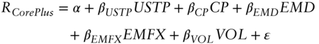
The average active (excess of benchmark) return is 1.18 percent (annualized) across all 142 funds. The average realized tracking error is 2.4 percent (annualized), leading to an average Sharpe ratio of 0.54. Impressive. For this analysis we have forced all funds to have the same benchmark: Bloomberg US Aggregate. The regression coefficients suggest meaningful positive exposure to the credit premium. The strength of that positive correlation is emphasized in the last column that shows the average correlation of active returns to credit premium, ![]() , is 0.72. Exhibit 4.5 shows a frequency histogram of this correlation coefficient across the 142 funds and Exhibit 4.6 shows a scatter plot of the monthly returns to the EW portfolio and credit premium. The strength of this passive beta capture is striking.
, is 0.72. Exhibit 4.5 shows a frequency histogram of this correlation coefficient across the 142 funds and Exhibit 4.6 shows a scatter plot of the monthly returns to the EW portfolio and credit premium. The strength of this passive beta capture is striking.
EXHIBIT 4.5 Relative frequency histogram of correlation between excess of benchmark (active) returns and credit premium returns ( ) for US Core Plus Funds.
Source: Bloomberg Indices, JP Morgan indices, and eVestment.

EXHIBIT 4.6 Scatter plot of equally weighted average US Core Plus fund excess of benchmark (active) returns and credit premium returns.
Source: Bloomberg Indices, JP Morgan indices, and eVestment.
Removing the effects of passive exposure to traditional market risk premia reduces the average active return of 1.18 percent to an “alpha” return of 0.41 percent, a reduction of 65 percent. To emphasize the broad‐based impact of how great an influence traditional market risk premia exposures have on the impressive active returns reported earlier, Exhibit 4.7 shows the relative frequency histograms of the annualized active returns and annualized alphas. The superimposed bell‐shaped curves are normal distributions with a zero average return and standard deviation equal to the sample return standard deviation. This easily allows the reader to see both the economic and statistical impact of passive beta exposure on estimated alphas. The bars are clearly far to the right of zero for active returns and much less so for alphas.

EXHIBIT 4.7 Relative frequency histograms of annualized active returns and annualized alphas for US Core Plus Funds.
Source: Bloomberg Indices, JP Morgan indices, and eVestment.
4.3 GLOBAL AGGREGATE BENCHMARKED FIXED INCOME MANAGERS
For our analysis of Global Aggregate benchmarked managers, we use the full universe of 108 active funds covered in the eVestment database under the “Global Aggregate” category as of the start of 2021. All active funds are retained for the analysis, and funds with less than 24 months of returns data are excluded. This leaves a final sample of 94 funds for the returns analysis that follows, and this reduced sample of funds covers 90 percent of the $355 billion USD covered in this category. All returns are gross of fees.
We run the following regression specification for each individual fund as well as for an equally weighted average across all funds. The period starts in January 1993 and runs through the end of 2020, and we use the full period available for each fund.
![]() is the monthly gross of fee return for the Global Aggregate benchmarked fund (or average across all Global Aggregate funds in a month). The right‐hand variables are all as defined in Exhibit 4.3. Exhibit 4.8 summarizes the regression analysis.
is the monthly gross of fee return for the Global Aggregate benchmarked fund (or average across all Global Aggregate funds in a month). The right‐hand variables are all as defined in Exhibit 4.3. Exhibit 4.8 summarizes the regression analysis.
EXHIBIT 4.8 Regression analysis for Global Aggregate Funds.
| Active Return | Sharpe Ratio | IR | ||||||||
|---|---|---|---|---|---|---|---|---|---|---|
| Q1 | 0.16% | 0.07 | −0.19 | −0.01 | −0.01 | −0.26 | −0.01 | −0.10% | −0.07 | 0.00 |
| AVG | 0.77% | 0.26 | −0.13 | 0.07 | 0.07 | 0.01 | 0.05 | 0.57% | 0.26 | 0.29 |
| Q2 | 0.77% | 0.27 | −0.04 | 0.07 | 0.05 | 0.03 | 0.04 | 0.52% | 0.19 | 0.38 |
| Q3 | 1.40% | 0.46 | 0.04 | 0.14 | 0.16 | 0.15 | 0.09 | 1.69% | 0.56 | 0.59 |
| EW portfolio | 0.93% | 0.42 | −0.06 | 0.06 | 0.07 | 0.03 | 0.02 | 0.23% | 0.19 | 0.60 |
Source: Bloomberg Indices, JP Morgan indices, and eVestment. Q1 (3) is first (third) quartile. AVG is average. Q2 is median. EW portfolio is the equally weighted average across all funds with nonmissing data each month. 1993–2020 period examined.
The average active (excess of benchmark) return is 0.77 percent (annualized) across all 94 funds. The average realized tracking error is 3.8 percent (annualized), leading to an average Sharpe ratio (excess of benchmark returns) of 0.26. For this analysis we have forced all funds to have the same benchmark: Bloomberg Global Aggregate. The regression coefficients suggest positive exposures to the credit premium, emerging market premium, and volatility premium. The average correlation of active returns to the credit premium, ![]() , is 0.29, considerably lower than what was seen for the Core Plus category. Exhibit 4.9 shows a scatter plot of the monthly returns to the equally weighted (EW) portfolio and credit premium, and we can again see a pervasive passive credit beta capture.
, is 0.29, considerably lower than what was seen for the Core Plus category. Exhibit 4.9 shows a scatter plot of the monthly returns to the equally weighted (EW) portfolio and credit premium, and we can again see a pervasive passive credit beta capture.
Removing the effects of passive exposure to traditional market risk premia reduces the average active return of 0.77 percent to an “alpha” return of 0.57 percent, a reduction of 25 percent. Exhibit 4.10 shows the relative frequency histograms of the annualized active returns and annualized alphas. Again, it is easy to see the economic and statistical impact of passive beta exposure on estimated alphas. The bars shift to the left as you move from active returns to alphas, but the alphas for this category are still significant. The astute reader will notice that the reduction of alpha for the Global Aggregate category is less than shown in the original research of Brooks, Gould, and Richardson (2020). The analysis here covers a slightly longer period and uses monthly returns, whereas the original research had examined nonoverlapping three‐month periods. The purpose is not to replicate the original research, simply to note the pervasiveness of beta capture across fixed income categories.

EXHIBIT 4.9 Scatter plot of equally weighted (EW) average Global Aggregate fund excess of benchmark (active) returns and credit premium returns.
Source: Bloomberg Indices, JP Morgan indices, and eVestment.

EXHIBIT 4.10 Relative frequency histograms of annualized active returns and annualized alphas for US Core Plus Funds.
Source: Bloomberg Indices, JP Morgan indices, and eVestment.
4.4 UNCONSTRAINED BOND FUNDS
For our analysis of Global Unconstrained Bond funds, we use the full universe of 113 active funds covered in the eVestment database under the “‘Global Aggregate” category as of the start of 2021. All active funds are retained for the analysis, and funds with less than 24 months of returns data are excluded. This leaves a final sample of 103 funds for the returns analysis that follows, and this reduced sample of funds covers 90 percent of the $450 billion USD covered in this category. All returns are gross of fees.
We run the following regression specification for each individual fund as well as for an equally weighted average across all funds. The period starts in November 1997 and runs through the end of 2020, and we use the full period available for each fund. The inclusion of the inflation risk premium shortens the sample by four years (Bloomberg Indices for inflation‐linked securities started in 1997).
![]() is the monthly gross of fee return for the Global Unconstrained Bond fund (or average across all Global Unconstrained Bond funds in a month). The right‐hand variables are all as defined in Exhibit 4.3. Exhibit 4.11 summarizes the regression analysis.
is the monthly gross of fee return for the Global Unconstrained Bond fund (or average across all Global Unconstrained Bond funds in a month). The right‐hand variables are all as defined in Exhibit 4.3. Exhibit 4.11 summarizes the regression analysis.
EXHIBIT 4.11 Regression analysis for Unconstrained Bond Funds.
| Active Return | Sharpe Ratio | IR | |||||||||
|---|---|---|---|---|---|---|---|---|---|---|---|
| Q1 | 2.14% | 0.34 | 0.27 | −0.23 | 0.13 | −0.20 | 0.03 | −0.05 | −0.58% | −0.17 | 0.54 |
| AVG | 4.09% | 0.74 | 0.65 | −0.21 | 0.39 | −0.01 | 0.40 | 0.07 | 0.57% | 0.34 | 0.63 |
| Q2 | 3.76% | 0.70 | 0.47 | −0.06 | 0.34 | 0.02 | 0.13 | 0.03 | 0.47% | 0.18 | 0.68 |
| Q3 | 4.99% | 1.03 | 0.86 | 0.02 | 0.61 | 0.15 | 0.71 | 0.11 | 1.61% | 0.55 | 0.80 |
| EW port. | 5.29% | 1.03 | 0.68 | −0.05 | 0.37 | 0.01 | 0.36 | 0.04 | −0.06% | −0.03 | 0.72 |
Source: Bloomberg Indices, JP Morgan indices, and eVestment. Q1 (3) is first (third) quartile. AVG is average. Q2 is median. EW portfolio is the equally weighted average across all funds with nonmissing data each month. 1997–2020 period examined.
The average active (excess of benchmark) return is 4.09 percent (annualized) across all 103 funds. The average realized tracking error is 6.9 percent (annualized), leading to an impressive average Sharpe ratio (excess of benchmark returns) of 0.74. For this analysis we have forced all funds to have the same benchmark: US cash rates (T‐bill returns). The regression coefficients suggest strong positive exposures to the term premium, credit premium, and emerging market currency premium. The average correlation of active returns to credit premium, ![]() , is 0.63. Exhibit 4.12 shows a scatter plot of the monthly returns to the EW portfolio and credit premium, and we can again see a pervasive passive credit beta capture.
, is 0.63. Exhibit 4.12 shows a scatter plot of the monthly returns to the EW portfolio and credit premium, and we can again see a pervasive passive credit beta capture.
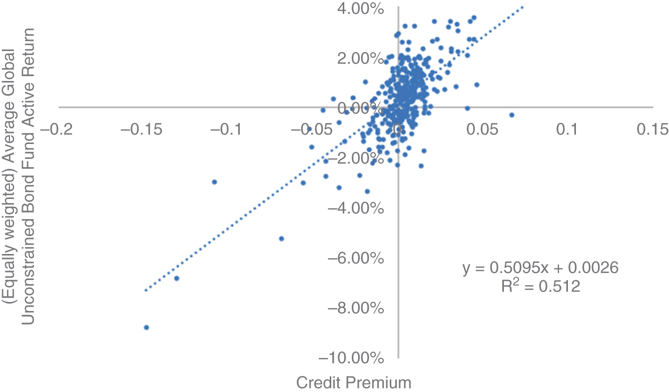
EXHIBIT 4.12 Scatter plot of equally weighted average Global Unconstrained Bond fund excess of benchmark (active) returns and credit premium returns.
Source: Bloomberg Indices, JP Morgan indices, and eVestment.
Removing the effects of passive exposure to traditional market risk premia reduces the average active return of 4.09 percent to an “alpha” return of 0.57 percent, a reduction of 85 percent. Exhibit 4.13 shows the relative frequency histograms of the annualized active returns and annualized alphas. Again, it is very easy to see the economic and statistical impact of passive beta exposure on estimated alphas. The bars shift to the left as you move from active returns to alphas, and in this case the “alphas” are very small compared to reported active returns. This is one category of active fixed income management in which the repacking of beta as alpha is both very large and very pervasive.
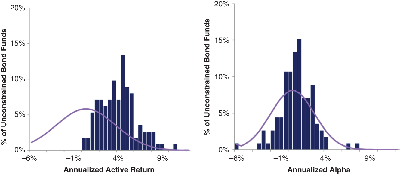
EXHIBIT 4.13 Relative frequency histograms of annualized active returns and annualized alphas for Global Unconstrained Bond Funds.
Source: Bloomberg Indices, JP Morgan indices, and eVestment.
4.5 EMERGING MARKET FIXED INCOME MANAGERS
For our analysis of emerging market bond funds, we use the full universe of 131 active funds covered in the eVestment database under the “‘Global Aggregate” category as of the start of 2021. All active funds are retained for the analysis and funds with less than 24 months of returns data are excluded. This leaves a final sample of 117 funds for the returns analysis that follows, and this reduced sample of funds covers 98 percent of the $355 billion USD covered in this category. All returns are gross of fees.
We run the following regression specification for each individual fund as well as for an equally weighted average across all funds. The period starts in February 2003 and runs through the end of 2020, and we use the full period available for each fund. The inclusion of the emerging corporate risk premium shortens the sample by a further six years (Bloomberg Indices for emerging corporate securities started in 2003).

![]() is the monthly gross of fee return for the emerging market bond fund (or average across all emerging market bond funds in a month). The right‐hand variables are all as defined in Exhibit 4.3. Exhibit 4.14 summarizes the regression analysis.
is the monthly gross of fee return for the emerging market bond fund (or average across all emerging market bond funds in a month). The right‐hand variables are all as defined in Exhibit 4.3. Exhibit 4.14 summarizes the regression analysis.
The average active (excess of benchmark) return is 1.04 percent (annualized) across all 117 funds. The average realized tracking error is 3.66 percent (annualized), leading to an average Sharpe ratio (excess of benchmark returns) of 0.29. For this analysis we have forced all funds to have the same benchmark: the Bloomberg Emerging Market USD Aggregate Index. The regression coefficients suggest positive exposures to the emerging market premium and to a lesser extent the volatility premium. The average correlation of active returns to credit premium, ![]() , is 0.26, lower than what was seen for the core‐plus and unconstrained categories.
, is 0.26, lower than what was seen for the core‐plus and unconstrained categories.
EXHIBIT 4.14 Regression analysis for Global Aggregate Funds.
| Active Return | Sharpe Ratio | IR | |||||||
|---|---|---|---|---|---|---|---|---|---|
| Q1 | 0.25% | 0.09 | −0.25 | 0.00 | −0.10 | −0.07 | −0.23% | −0.11 | −0.03 |
| AVG | 1.04% | 0.29 | −0.12 | 0.11 | 0.04 | 0.07 | 0.54% | 0.23 | 0.26 |
| Q2 | 0.95% | 0.29 | −0.12 | 0.15 | 0.03 | 0.07 | 0.49% | 0.20 | 0.33 |
| Q3 | 1.65% | 0.48 | 0.02 | 0.25 | 0.16 | 0.18 | 1.17% | 0.53 | 0.55 |
| EW portfolio | 4.01% | 0.87 | −0.15 | 0.11 | −0.05 | 0.13 | 0.87% | 0.65 | 0.21 |
Source: Bloomberg Indices, JP Morgan indices, and eVestment. Q1 (3) is first (third) quartile. AVG is average. Q2 is median. EW portfolio is the equally weighted average across all funds with nonmissing data each month. 2003–2020 period examined.
Removing the effects of passive exposure to traditional market risk premia reduces the average active return of 1.04 percent to an “alpha” return of 0.54 percent, a reduction of just over 50 percent. Exhibit 4.15 shows the relative frequency histograms of the annualized active returns and annualized alphas. Again, it is easy to see the economic and statistical impact of passive beta exposure on estimated alphas, with the bars shifting to the left as you move from active returns to alphas.

EXHIBIT 4.15 Relative frequency histograms of annualized active returns and annualized alphas for Emerging Market bond funds.
Source: Bloomberg Indices, JP Morgan indices, and eVestment.
4.6 CREDIT LONG/SHORT MANAGERS
For an analysis of credit hedge funds, we need to use a different data source. We will use the same data source as Palhares and Richardson (2020) – namely, Hedge Fund Research Indices (HFRI) (HFR database). For the time‐series analysis examining the beta and systematic exposures of actively managed credit hedge funds, we use the HFRI Relative Value: Fixed Income: Corporate Index. The data analysis spans the 1996–2020 period. We limit ourselves to individual funds within this HFR category that are current constituents of the index as of 2021. This leaves a sample of 51 live credit hedge funds. This sample size is smaller than the 219 credit hedge funds examined in Palhares and Richardson (2020), as they also looked at the “graveyard” funds. So although we have a smaller set of funds here, any evidence of positive risk‐adjusted returns will be positively biased due to survivorship (they are all live funds). That bias is fine for our purposes, as we wish to explore the extent to which passive beta exposure can explain credit hedge funds returns. All the returns data examined in this section are net of fee (so any excess of benchmark return for this category should be viewed as more impressive than the previous categories that were all gross of fee).
We run the following regression specification for each individual fund, as well as for an equally weighted average across all funds. The period starts in 1996 and runs through the end of 2020, and we use the full period available for each fund.
![]() is the monthly net‐of‐fee return for the credit long/short hedge fund (or average across all credit long/short hedge funds in a month). The right‐hand variables are based on those included in Palhares and Richardson (2020): (i) term premium (USTP), (ii) credit premium (CP), and (iii) equity risk premium (EP). The return analysis here, and for the regressions that follow, use nonoverlapping three‐month returns to account for the known staleness in pricing for both credit hedge funds and credit markets generally. The analyses in the prior sections used monthly returns. Exhibit 4.16 summarizes the regression analysis.
is the monthly net‐of‐fee return for the credit long/short hedge fund (or average across all credit long/short hedge funds in a month). The right‐hand variables are based on those included in Palhares and Richardson (2020): (i) term premium (USTP), (ii) credit premium (CP), and (iii) equity risk premium (EP). The return analysis here, and for the regressions that follow, use nonoverlapping three‐month returns to account for the known staleness in pricing for both credit hedge funds and credit markets generally. The analyses in the prior sections used monthly returns. Exhibit 4.16 summarizes the regression analysis.
The average active (excess of cash) return is 8.66 percent (annualized) across all 51 funds. The average realized tracking error is 10.23 percent (annualized), leading to an average Sharpe ratio (excess of benchmark returns) of 1.09, truly impressive (but keep in mind the survivorship bias with the use of only current live funds). The average Sharpe Ratio is computed across all funds, it is not the ratio of the average active return (8.66 percent) to the average tracking error (10.23 percent), the average of a ratio is not equal to the ratio of the averages. The regression coefficients suggest very positive exposures to the credit premium. The average (median) correlation of active returns to credit premium, ![]() , is 0.66 (0.79), and Exhibit 4.17 shows how pervasive this passive credit beta capture is across credit hedge funds (this result mirrors the strong evidence of equity beta included in equity long/short funds examined in Asness, Krail, and Liew 2001). Although there are a very small number of credit hedge funds with low or negative correlations to broad credit markets, most have large passive credit betas. And over the last decade, that has been a fabulous return source.
, is 0.66 (0.79), and Exhibit 4.17 shows how pervasive this passive credit beta capture is across credit hedge funds (this result mirrors the strong evidence of equity beta included in equity long/short funds examined in Asness, Krail, and Liew 2001). Although there are a very small number of credit hedge funds with low or negative correlations to broad credit markets, most have large passive credit betas. And over the last decade, that has been a fabulous return source.
EXHIBIT 4.16 Regression analysis for credit long/short hedge funds.
| Active Return | Sharpe Ratio | IR | ||||||
|---|---|---|---|---|---|---|---|---|
| Q1 | 6.15% | 0.64 | −0.09 | 0.43 | −0.05 | 1.40% | 0.27 | 0.62 |
| AVG | 8.66% | 1.09 | 0.17 | 0.69 | 0.02 | 3.85% | 0.76 | 0.66 |
| Q2 | 8.31% | 0.84 | 0.13 | 0.67 | 0.03 | 3.33% | 0.73 | 0.79 |
| Q3 | 9.67% | 1.13 | 0.36 | 0.99 | 0.13 | 6.20% | 1.27 | 0.91 |
| EW portfolio | 10.89% | 1.26 | 0.17 | 0.61 | 0.03 | 8.62% | 1.80 | 0.83 |
Source: Bloomberg Indices, MSCI indices, and HFR. Q1 (3) is first (third) quartile. AVG is average. Q2 is median. EW portfolio is the equally weighted average across all funds with nonmissing data each month. 1996–2020 period examined.
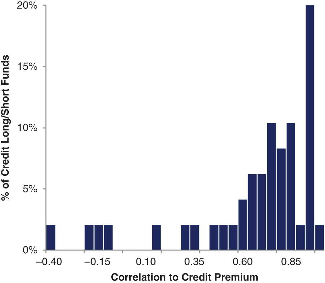
EXHIBIT 4.17 Relative frequency distribution of credit hedge fund correlation of net‐of‐fee returns and credit premium. Period 1996–2020.
Source: HFRI (HRF database) and Bloomberg Indices.
It is important to note that the use of the live set of credit hedge funds as of the end of the sample period means we are examining credit funds over a period in which the credit markets have delivered fantastic risk adjusted returns. Over the 1996–2020 period, the credit premium delivered a 2.6 percent annualized excess return with an annualized volatility of 10.2 percent (0.25 Sharpe ratio); however, over the 2010–2020 period the Sharpe ratio was 0.54 (4.5 percent annualized return). Why is this relevant? The set of 51 credit hedge funds we examine have an average (median) track record of 117 (110) months, which corresponds mostly to the 2010–2020 period. Credit hedge funds do have significant credit beta exposure, and this passive beta has generated a lot of the impressive net‐of‐fee returns.
Removing the effects of passive exposure to traditional market risk premia reduces the average excess of cash return of 8.66 percent to an “alpha” return of 3.85 percent, a reduction of over 55 percent. Exhibit 4.18 shows the side‐by‐side relative frequency histograms of annualized excess of cash returns and annualized alpha (both net of fees). The probability mass is very far to the right of zero. Again, formal econometric tests are hardly needed for Exhibit 4.18; every (still live) credit hedge fund has realized a (large) positive annualized return over 1996–2020.

EXHIBIT 4.18 Relative frequency histograms of annualized active returns and annualized alphas for credit long/short hedge funds.
Source: Bloomberg Indices, MSCI indices, and HFR.
Finally, Exhibit 4.19 shows the extent of this passive credit beta capture by credit hedge funds. This scatter plot shows a very strong relation between the average credit hedge fund return and contemporaneous credit excess returns for the US HY market (the full‐sample correlation is 0.83). This correlation to the credit premium is pervasive across funds. About half of the credit hedge fund net‐of‐fee returns is attributable to passive (credit) beta capture. Is that worth a 2/20 fee?
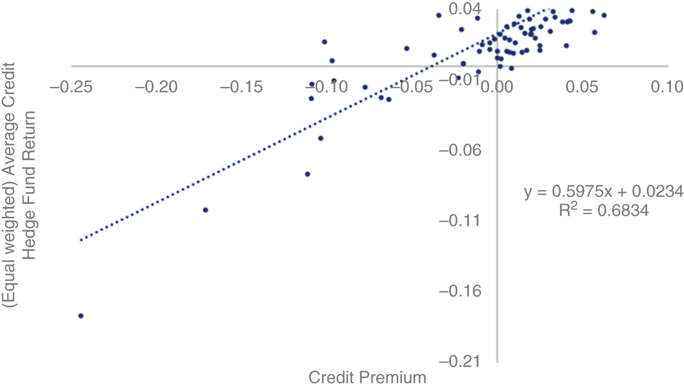
EXHIBIT 4.19 Scatter plot of (equal weighted) net‐of‐fee credit hedge fund return against US HY index credit excess returns. Period 1996–2020.
Source: HFRI (HRF database) and Bloomberg Indices.
In summary, this chapter has provided an in‐depth analysis of the excess of benchmark returns for a broad set of actively managed fixed income funds. There is a very strong general theme that emerges. There is a considerable allocation of active risk taking to passive beta exposures, especially to credit risk. Although estimated alphas are considerably smaller than active returns across all fixed income categories examined, there is still alpha to be found through active fixed income management. The magnitude of that alpha is significantly less than that suggested by a simple analysis of excess of benchmark returns. Asset owners are aware of reaching for yield behavior but may not fully appreciate either the pervasiveness of this behavior or how large an impact it can have on returns.
The challenge for systematic fixed income investing is to harness the investment opportunity set within fixed income, including (i) avoiding bad‐selling practices, (ii) asset allocation decisions, (iii) out of benchmark tilts, (iv) liquidity provision, and (v) security selection. We have seen how challenging tactical asset allocation is (Chapter 3) and how pervasive passive credit beta capture is for fixed income managers. For the next three chapters we will focus on the return potential from security selection sources within rate‐sensitive bonds (Chapter 5), credit‐sensitive bonds (Chapter 6) and emerging‐market bonds (Chapter 7). Let's hope we can generate excess of benchmark returns (a necessary condition for successful active fixed income management) and do so with low correlations to traditional market risk premia. If we can manage both, systematic fixed income investing will be highly valuable for asset owners. As we will see in our concluding chapter, I believe this diversification benefit of systematic investing approaches can be realized.
REFERENCES
- Asness, C., R. Krail, and J. Liew. (2001). Do hedge funds hedge? Journal of Portfolio Management, 28, 6–19.
- Baz, J., R. Mattu, J. Moore, and H. Guo. (2017). Bonds are different: Active versus passive management in 12 points. PIMCO Quantitative Research.
- Ben Dor, A., A. Desclee, L. Dynkin, J. Hyman, and S. Polbennikov. (2021). Systematic Investing in Credit. Wiley.
- Brooks, J., T. Gould, and S. Richardson. (2020). Active fixed income illusions. Journal of Fixed Income, 29, 5–19.
- Brooks, J., S. Richardson, and Z. Xu. (2020). (Systematic) Investing in emerging market debt. Journal of Fixed Income, 30, 44–61.
- Ilmanen, I. (2011). Expected Returns. Wiley.
- Palhares, D., and S. Richardson. (2020). Looking under the hood of active credit managers. Financial Analysts Journal, 76, 82–102.